Estimation of Endogenous Volatility Models with Exponential Trends

Abstract

Nonlinearities, exponential trends, and Euler equations are three key features of standard dynamic volatility models of speculation, economic growth, or macroeconomic fluctuations with occasionally binding constraints and endogenous state-dependent volatility. A natural way to estimate a model with all such three features could be to use the observed nonstationary data in a single step without preliminary linearization, log-linearization, or preliminary detrending. Adoption of this natural strategy confronts a serious challenge that has been neither articulated nor solved: a dichotomy in the empirical model implied by the Euler equation. This leads to a discontinuity in the regression in the limit, rendering the approaches employed in available proofs of consistency inapplicable. We characterize the problem and develop a novel method of proof of consistency and asymptotic normality. Our methodological contribution establishes a foundation for consistent estimation and hypothesis testing of nonstationary models without resorting to preliminary detrending, an a priori assumption that any trend is exactly zero, linearization, or other restrictions on the model.

1. Introduction

Dynamic stochastic problems of asset accumulation and allocation subject to random shocks and occasionally binding constraints (for example, non-negativity constraints or limits on asset decumulation or aggregate borrowing) are important in numerical studies of commodity price volatility, macroeconomic fluctuations, and economic growth. Empirical analysis of such problems encounters significant challenges. We illustrate these in a simple model of price volatility in a market for a storable commodity such as grain that is our main focus here. The market includes an exponential positive trend in productivity, a random harvest shock, a non-negativity constraint on stocks, and Euler equations for deriving profit-maximizing storage decisions. These features are shared by many dynamic stochastic models of speculation, economic growth, or macroeconomic fluctuations with occasionally binding constraints and endogenous state-dependent volatility (see for example [1,2,3,4,5], and references therein).

A natural way to estimate models with such features could be to implement the estimation of nonlinear Euler equations using the nonstationary observed data and letting the data reveal estimates of trends and other parameters relevant to the volatility of prices or other measures of value.

Even in our simple commodity market model, the exponential trend in the dependent variable (for example, price of a storable commodity) poses a challenge to identification first discussed in the context of a simple first-order decay model [6].

Standard representation of the Euler equation normalized by the current (unknown) estimated value of the exponential trend solves this identification problem. However, if the aim is to estimate the value of at least one other parameter besides the trend, use of this normalization introduces a serious obstacle: a dichotomy in the empirical model implied by the Euler equation when the estimated trend parameter is in the neighborhood of its true value. This implies a discontinuity in the regression in the limit, rendering the approaches employed in available proofs of consistency inapplicable.

Studies that estimate parameters of models involving similar challenges generally take one of four currently prevalent approaches. The first is to ignore any trend as negligible (see for example [7,8,9,10,11,12,13]), another is the common practice of resorting to linearization or log-linearization of Euler equations implied by inter-temporal arbitrage (which might well mis-specify the incentives implied by the model) (see [14,15,16] for discussions of the serious implications of such mis-specifications), a third is de-trending of the data prior to estimation using the mean value of an exponential trend estimated on the data in a preliminary step (see [2,17,18]), and a fourth is de-trending the data simultaneously with the estimation of all other unknown parameters but ignoring the endogenous interaction of the trend and economic incentives in the Euler equation (see for example [1,3,19]).

Each of these approaches restricts the information that can be revealed in empirical analysis. How important are these restrictions? It has been difficult to address this question in the absence of a less restrictive approach that can be used for comparison.

We offer such a less restrictive approach—a one-step procedure to estimate all parameters simultaneously—to minimize the sum of squared residuals of the estimated nonlinear Euler equations, recognizing the interaction of an exponential trend in price with the endogenous economic incentives implied by the model.

We use nonlinear least squares which, as Wu [20] notes in his classic paper, has a central role in inference of parameters in nonlinear regression models. Wu [20] further notes that such inference is necessarily asymptotic but that much of the work prior to his paper focuses on problems such as asymptotic normality, avoiding the “harder problem” of consistency by assuming that it holds.

We address the key problem of consistency of our estimator in line with the suggestion of [21] (p. 1050) to focus on extending asymptotic analysis to cases where the forcing variables are not necessarily stationary but have a time invariant representation.

Although exponential trends are commonly used in nonstationary dynamic models, the regressions implied by the Euler equations of the models we consider do not satisfy the sufficient conditions for consistency of estimators available in the literature. In particular, the uniform convergence condition in [22], the Lipschitz condition of [20], the Lipschitz conditions of [23], the continuity-type smoothness conditions of [24,25], the differentiability conditions of [26], and the stochastic Lipschitz conditions in [27] do not hold.

Article [28] established consistency and central limit theorems for models where the unobserved errors are independent, as assumed in [20,29]. In contrast, and in line with most of the empirical literature on nonlinear dynamic economic models, we consider cases where the residuals are Markovian and not independent.

To the best of our knowledge, in the four decades since [21] there has been no study that provides asymptotic theory for the estimation of nonstationary nonlinear dynamic stochastic models of intertemporal arbitrage of the type we consider here. These models include an unknown exponential trend in the structure of the predictor that interacts with at least one other parameter and do not have independent errors.

In what follows, we address estimation of key parameters of economic models with endogenous volatility. The ability to test the assumption that any secular trend in the endogenous variable of interest is exactly zero is potentially important for tests of other parameters affecting dynamic stochastic behavior. Our main focus is on a dynamic stochastic model of commodity price behavior of a storable commodity such as wheat described in detail in [2]. This model is a nonstationary extension of the classic stationary model of speculative arbitrage with occasionally binding non-negativity constraints on inventories in the tradition of [30,31,32]. This model is highly relevant to current concerns with price prediction in markets with high and volatile commodity prices.

We develop a novel method of proof of consistency and asymptotic normality for such models. Thus, we establish a foundation for estimation and hypothesis testing, without

(i)

Ignoring the possibility of a secular trend,

(ii)

Using prior detrending,

(iii)

Assuming linear or log-linear Euler equations,

(iv)

Ignoring the possible interaction of a trend and other parameters in the Euler equation,

(v)

Assuming independent errors.

In Section 2, we present a background for the problem we solve. Then, in Section 3, we present our main example, the commodity storage model. In Section 4 and Section 5, we present our proofs of identification, consistency, and asymptotic normality for this nonstationary model of speculative arbitrage of consumable commodity inventories with occasionally binding non-negativity constraints in the tradition of [30,31,32].

We then, in Section 6, show how our proofs can be applied to two empirical models of economic growth. The presentation of our results for such models is brief, since we discuss the same methodological challenge and use the same techniques as for the commodity storage model. The model in Section 6.1 is a non-stationary version of the growth model of [33], which, like many DSGE models, presents the additional challenge that the predictor in the regression is unbounded. In Section 6.2, we address estimation of a two-sector empirical growth model with occasionally binding constraints in capital.

In Section 7, we present numerical simulations of our results for the storage model in Section 3; in Section 8, we offer concluding remarks.

2. Preliminaries

In this section, we discuss the estimation problem and a general presentation of our approach to solving it.

The types of models we address include intertemporal Euler equations that imply regressions of the form:

$${\displaystyle Y_{t+1}=f(t,x_t,{\theta }_0)+{ϵ}_{t+1}}$$

(1)

where $t\in \mathbb{N}$ is time, ${\theta }_0\in \Theta$ is the vector of the unknown true values of at least two parameters, one of which is the exponential trend parameter, $\Theta$ is a compact set in ${\mathbb{R}}^q,$$x_t$ is a regressor, and ${\left\{{ϵ}_{t+1}\right\}}_{t\in \mathbb{N}}$ is a martingale difference sequence.

We present our results in the familiar setting of nonlinear least squares estimation although our approach can be more broadly applied. In the standard case [22], the average of squared residuals $\frac{1}{T}{\sum }_{t=1}^T{(Y_{t+1}-f(t,x_t,\theta ))}^2$ is uniformly convergent in $\theta \in \Theta .$

In the models we consider, this average is pointwise convergent for $\theta \in \Theta .$ However, the presence of a quite standard exponential trend in the driving process implies that such convergence is not uniform.

Our proof of strong consistency of the least squares estimator of ${\theta }_0$ is based on the proof of the following uniform strong law of large numbers:

$${\displaystyle {\lim }_{T\to \infty }\frac{1}{A_T}\underset{\theta \in B\left(\mu \right)}{sup}\left|\sum _{t=1}^T{ϵ}_{t+1}\{f(t,x_t,\theta )-f(t,x_t,{\theta }_0)\}\right|=0,\mathrm{almost} \mathrm{surely}}$$

(2)

where $\mu \ne {\theta }_0$, $B\left(\mu \right)$ is a ball centered at $\mu$ with ${\theta }_0\notin B\left(\mu \right)$, and

$$A_T\equiv {\inf }_{\theta \in B\left(\mu \right)}\sum _{t=1}^T{\{f(t,x_t,\theta )-f(t,x_t,{\theta }_0)\}}^2.$$

(For papers that prove similar uniform laws of large numbers for other regression models, see for example [20] Lemma 1, p. 504, [26] p. 1927, and [27] pp. 878–879).

The regression models considered in this paper imply a new challenge for the proof of (2). Specifically, for the commodity storage model we present in Section 3, the predictor f in (1) is a function of ${(\lambda /{\lambda }_0)}^t$ where t is time, $\lambda >0$ is a value of the trend parameter in the ball $B\left(\mu \right)$, and ${\lambda }_0>0$ is the true (unknown) value of the trend parameter.

More precisely, for the storage model,

$${\displaystyle Y_{t+1}=f(t,p_t,\theta )+{ϵ}_{t+1}=\gamma min\left\{{\left(\frac{\lambda }{{\lambda }_0}\right)}^t\frac{p^{*}}{p_t},1\right\}+{ϵ}_{t+1}.}$$

where $p_t$ is a regressor, and $\theta =(\lambda ,p^{*},\gamma )$ is a vector of strictly positive estimated parameter values. The term ${(\lambda /{\lambda }_0)}^t$ has a dichotomy when $\lambda$ passes through ${\lambda }_0.$ Indeed, if $(\lambda /{\lambda }_0)<1,$ then ${(\lambda /{\lambda }_0)}^t$ decreases exponentially with $t.$ In contrast, if $(\lambda /{\lambda }_0)>1,$ then ${(\lambda /{\lambda }_0)}^t$ increases exponentially with $t.$ This dichotomy induces a discontinuity in ${\lim }_{t\to \infty }f(t,p_t,\theta ).$

If ${\lambda }_0$ and at least one other parameter are unknown, the proof of (2) is not necessarily immediate. 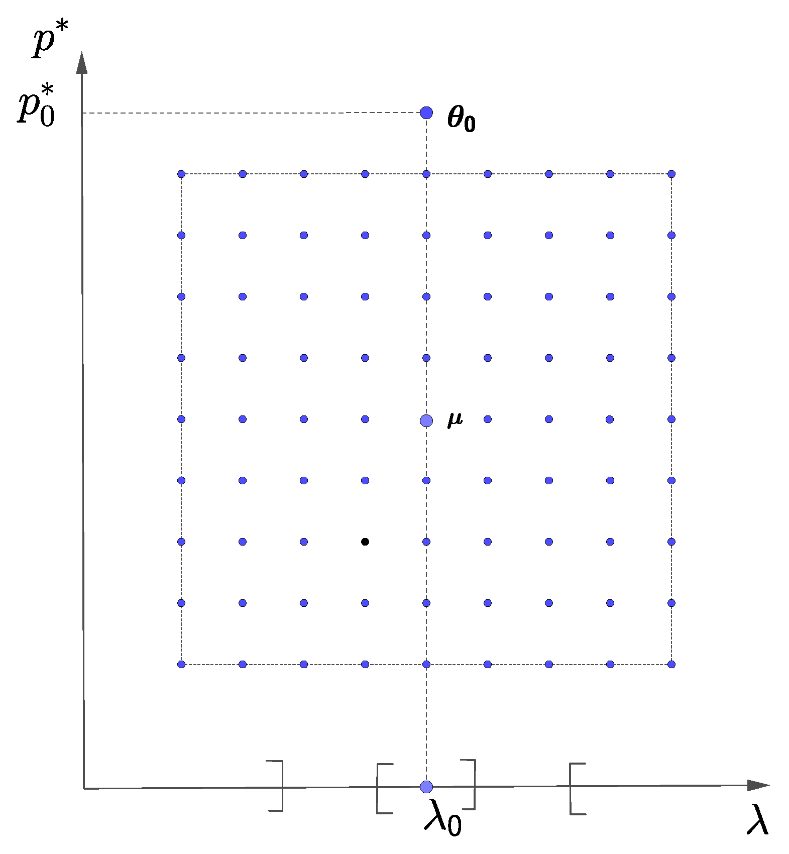In the nontrivial case, the ball $B\left(\mu \right)$ in (2) includes ${\lambda }_0$ and values of $\lambda$ that are strictly less than ${\lambda }_0,$ and other values for $\lambda$ that are strictly greater than ${\lambda }_0.$ This implies that the discontinuity in ${\lim }_{t\to \infty }f(t,p_t,\theta )$ can occur in the interior of the ball $B\left(\mu \right)$ in (2). For simplicity, such a ball is illustrated in two dimensions by the square ball in Figure 1, where we denote the other parameter as $p^{*},$ and $p_0^{*}$ is its unknown true value.

Figure 1. A square ball in the parameter space.

Were ${\lambda }_0$ the only unknown, the ball $B\left(\mu \right)$ would not include ${\lambda }_0$, simplifying the proof of (2). Indeed, the ball $B\left(\mu \right)$ would be an open interval strictly to the left or to the right of ${\lambda }_0$, as illustrated by the alternate open intervals on the horizontal axis of Figure 1. We shall refer to the dots in Figure 1 when discussing the proof of Theorem 2 below, which makes use of sequences of arrays of discrete points such as the array for the square ball illustrated in Figure 1.

The function f is such that small deviations in $\lambda$ from ${\lambda }_0$ can induce large deviations in the estimates of the other parameters. The presence of ${(\lambda /{\lambda }_0)}^t$ in the predictor f implies that the trend parameter estimator must be superconsistent if the estimators of the other unknown parameters are to be consistent.

In our proof of (2), we use Azuma’s Lemma for martingale difference sequences [34], to show that the predictor f and its slope have a bound of polynomial order which we prove is killed by a negative exponential bound, uniformly on $\theta \in \Theta .$

In what follows, we address estimation of key parameters of three types of economic models with endogenous volatility in which the ability to test the assumption that any secular trend in the endogenous variable of interest is exactly zero is potentially important for tests of other parameters affecting dynamic stochastic behavior. Our main focus is on estimation of a dynamic stochastic model of commodity price behavior, addressed in Section 3. This model is most relevant to the current concern with high and volatile prices of storable commodities.

3. Speculative Commodity Storage

3.1. Overview

We consider a model of the market for a storable commodity with nonstationary supply described in [2]. For our paper to be self-contained, we present in this subsection a brief description of the simple market model described in greater detail in [2].

The model includes a stationary consumer demand with negative response to price and no response to changes in income. Production is a random harvest with a secular increasing trend. If the harvest is large and price is low, a portion of the output can be stored by speculators who maximize expected profit, selling some or all of their inventories when the price is higher subject to the constraint that stocks cannot be negative.

The dynamic behavior of this model alternates between two regimes. In one, the current price is sufficiently high that stocks are zero. In this “stockout” regime, we assume that the functional form of the latent consumption demand and the nature of the production process are such that their interaction implies a price target that follows a deterministic log-linear trend $\lambda >0.$ This target is an attractor; it is the conditional price expectation when current stocks are zero and arbitrage is not active. In this regime, price is volatile; the effects of harvest shocks on price are not buffered by currently available stocks. The expected price change is a “jump” to the trending attractor.

In the alternate regime, the current price is sufficiently low that stocks are positive. Intertemporal storage arbitrage ensures that the expected price exceeds the current observed price by the interest cost accrued on a one period investment in one unit of the commodity, which is the sole cost of storage. In this regime, price is less volatile and follows a stochastic trend; the attractor following the deterministic secular trend is latent until stocks revert to zero.

3.2. The Model

There is a representative consumer with stationary inverse consumption demand for the commodity $F,$ with $P_t=F\left(C_t\right),$ where $P_t$ and $C_t$ denote the observed price and consumption at time t, which we denote as “trending price” and “trending consumption,” respectively, where “trending” means “in the model with an exogenous production trend”. We assume the inverse demand function F to be stationary and strictly decreasing.

Rather than following the literature and specifying a particular functional form for F, we assume that it is in a general class of demand functions for a consumer whose utility function is in the Homothetic Absolute Risk Aversion (HARA) class (see [35] for details about the HARA utility functions). Such demand functions are characterized by:

$${\displaystyle \frac{F^{″}F}{{\left(F^{\prime }\right)}^2}=\kappa ,}$$

(3)

where $\kappa$ is a constant. This specification is not very restrictive: it includes, for example, the popular linear, log-linear, and iso-elastic consumption demand functions as particular cases.

Like previous models of storage with positive probability of stockouts (periods with no stocks) in the tradition of [30], we assume no convenience yield. (That is, we rule out storage at apparently negative net expected return.) Indeed, there is no storage cost apart from a constant interest rate $r>0.$

Total available supply at time t is $Z_t$. Competitive storers choose non-negative aggregate stocks $X_t\equiv Z_t-C_t\ge 0$, to maximize expected profits

$$\left[\frac{1}{1+r}{E}_t{P}_{t+1}-P_t\right]X_t,$$

where $E_t$ denotes expectation conditional on information at time t. If current stocks $X_t$ are positive:

$$E_t{P}_{t+1}=(1+r)P_t.$$

Note that in this regime with positive stocks the short-run “spread” $r{P}_t$ between the expected price in the next period and the current price is independent of the secular trends in production and price.

If the expected price is bounded, positive stocks $X_t$ go to zero in finite time, inducing a switch in the price regime. Hence the price is determined by the following nonlinear condition:

$$F\left(C_t\right)=max\left[F\left(Z_t\right),\frac{1}{1+r}{E}_{t}F\left(C_{t+1}\right)\right],$$

(4)

subject to

$$Z_{t+1}\equiv Z_t-C_t+H_{t+1},\forall t\in \mathbb{N},$$

(5)

conditional on initial $Z>0,$ where $H_{t+1}$ and $Z_{t+1}$ denote production and total available supply at time $t+1$, respectively.

We assume that production $H_t$ is given implicitly by $F\left(H_t\right)={\lambda }^{t}F\left(h_t\right),$ where “normalized production” $h_t$ is $i.i.d.$, with compact support $[\underline{h},\overline{h}],$$0\le \underline{h}<\overline{h}<\infty ,$ satisfying $F\left(\overline{h}\right)>0,$ and that the distribution of $h_t$ is absolutely continuous, with a continuous and strictly positive derivative on the interior of its support. To rule out bubble models, we assume ${\displaystyle EF\left(h\right)<\infty ,}$ where E denotes the expectation with respect to $h.$ (For discussions of bubble models of storage arbitrage, see for example [36,37,38]).

Normalized available supply $z_t$ and normalized consumption $c_t$ are defined implicitly in terms of their trending counterparts by the equations ${\lambda }^{t}F\left(z_t\right)=F\left(Z_t\right)$, ${\lambda }^{t}F\left(c_t\right)=F\left(C_t\right).$ Then, the stationary counterparts of Equations (4) and (5) are:

$$F\left(c_t\right)=max\left[F\left(z_t\right),\frac{\lambda }{1+r}{E}_{t}F\left(c_{t+1}\right)\right],$$

(6)

subject to

$$z_{t+1}\equiv {\lambda }^{\kappa -1}(z_t-c_t)+h_{t+1}.$$

(7)

We define $p_t\equiv F\left(c_t\right)$. We denote $p_t$ the “detrended” price, with some abuse of terminology. In general, $p_t$ is not the price process if $\lambda \equiv 1$; indeed the trend parameter affects the storage incentive in the normalized model and thus affects the amount of stocks, the timing of regimes, and the detrended prices. Note that $\lambda$ appears in the normalized model described by Equations (6) and (7).

Given $\lambda <1+r,$ a standard argument (see for example the proof of Theorem 1 in [7]) implies the existence of a Stationary Rational Expectations Equilibrium (SREE) function $p:[\underline{h},\infty )\to \mathbb{R}$ for the detrended price:

$${\displaystyle p_t=p\left(z_t\right)=max\left[F\left(z_t\right),\frac{\lambda }{1+r}{E}_{t}p\left(z_{t+1}\right)\right].}$$

(8)

Moreover, p is non-negative, continuous, and strictly decreasing if strictly positive. The following complementary inequalities hold:

$$\begin{array}{cc}p\left(z\right)=F\left(z\right),\hfill & \mathrm{for}z\le F^{-1}\left(p^{*}\right),\hfill \\ p\left(z\right)>F\left(z\right),\hfill & \mathrm{for}z>F^{-1}\left(p^{*}\right),\hfill \end{array}$$

where ${\displaystyle p^{*}\equiv \frac{\lambda }{1+r}Ep\left(h\right)\in \mathbb{R}.}$

Equation (8) implies the autoregression for detrended prices:

$${\displaystyle E_t{p}_{t+1}=\left(\frac{1+r}{\lambda }\right)min[p^{*},p_t].}$$

(9)

In terms of observed “trending” prices, the equivalent autoregression is:

$$E_t{P}_{t+1}=(1+r)min[{\lambda }^t{p}^{*},P_t].$$

(10)

The trend in the price target $(1+r){\lambda }^t{p}^{*}$ in Equation (10) is induced by the interaction of the latent production trend and the latent consumer demand of the HARA class.

Since $P_t=F\left(C_t\right)={\lambda }^{t}F\left(c_t\right)$ and the detrended price is given by $p_t=F\left(c_t\right)$, we have $P_t={\lambda }^t{p}_t$. Note that in the regime with positive stocks, the Euler equation implies that the expected trending price increases at the interest rate, $E_t{P}_{t+1}-P_t=r{P}_t$, regardless of the trend. In this regime, detrended price increases in expectation at a rate higher than r to compensate for the trend, as indicated in Equation (9).

The asymptotic theory for estimation presented in Section 4 and Section 5 below exploits the ergodic properties of the detrended price $p_t,$ which we now address.

The process for normalized available supply $\Phi \equiv {\left\{z_t\right\}}_{t\ge 0}$ is Markov, as proved in [2]. Indeed, since p is strictly decreasing (and therefore injective) whenever it is strictly positive and our assumption $F\left(\overline{h}\right)>0$ implies that the minimum detrended price in the state space, $\underline{p}=p\left(\overline{z}\right),$ is strictly positive, we conclude that the detrended price process is an injective mapping of a Markov process. This implies that detrended prices and ${\left\{p_t\right\}}_{t\ge 0},$$p_t=p\left(z_t\right),$ form a Markov process. (See [2] for more details.)

Given that the Markov process $\Phi \equiv {\left\{z_t\right\}}_{t\ge 0}$ is aperiodic on a compact state space and a geometric drift condition towards a petite set holds, [2] (Theorem 2) proves that the Markov process of normalized available supply $\Phi \equiv {\left\{z_t\right\}}_{t\ge 0}$ is uniformly ergodic. Thus, it has a unique invariant probability measure ${\nu }_{\infty }$ that is a global attractor, and there exist constants $k>1$ and $R<\infty$ such that for any initial normalized available supply $z_0,$ we have:

$$\left|\right|{\nu }_t-{\nu }_{\infty }\left|\right|\le R{k}^{-t},$$

where $\left|\right|·\left|\right|$ denotes the total variation norm, and ${\nu }_t$ is the distribution on $z_t$ conditional on initial detrended available supply.

4. Strong Consistency of Estimators

For the storage model discussed in the previous section, the estimation procedure in [2] involves two steps. In a preliminary step, the exponential trend on the observed prices and time is estimated and the point estimate of the trend is used to "de-trend" the prices. In the second step, conditional on the point estimate of the trend parameter, estimate behavioral parameters related to short run arbitrage. In contrast, here we propose estimation of all key parameters of the model in a single step.

Given data on prices and time only, in this section we prove strong consistency of nonlinear least squares estimation of three key parameters of the model: the trend parameter, $\lambda ,$ the detrended price threshold, $p^{*},$ and the interest rate, $r.$ For clarity of exposition, in the remainder of this section and in the following section we write a subscript “0” to denote the true parameter values. ${\theta }_0\equiv ({\lambda }_0,p_0^{*},{\gamma }_0),\mathrm{where}{\gamma }_0\equiv 1+r_0.$

Our empirical model is based in the threshold nonlinear price autoregression (10). The presence of an exponential trend in the threshold affects the regression predictor; in fact our empirical model violates key assumptions of continuous threshold models (see [39] for a survey), including continuity of the regression in the limit.

Price changes have two distinct volatility regimes that are recurrent, a feature which is useful for the implementation of our estimation approach. In one regime, intertemporal arbitrage is not active, stocks are zero, and the predictor in regression (1) is a function of calendar time and of the trend parameter. In the other regime, intertemporal arbitrage is active, the expected relative price change equals the interest rate, and the predictor in (1) is independent of the trend parameter. This second regime allows us to bound the predictor in the regression and its slope with a bound of polynomial order which, using Azuma’s Lemma [34], we prove is killed by a negative exponential bound.

For our asymptotic theory, we assume that the invariant distribution for the detrended price process has support $[\underline{p},\overline{p}],$ with $0<\underline{p}<p^{*}<\overline{p}<\infty .$ (For linear consumption demand, [40] derives a finite upper bound $\overline{h}$ to guarantee $p_t\ge \underline{p}>0,$ for all t).

Equation (10) implies:

$${\displaystyle P_{t+1}={\gamma }_{0}min\left\{{\lambda }_0^t{p}_0^{*},P_t\right\}+e_{t+1},\mathrm{where}{E}_t\left(e_{t+1}\right)=0.}$$

(11)

We assume that the parameter space $\Theta$ is compact.

Our objective is to estimate ${\theta }_0$ using least squares. Note that if $0<{\lambda }_0<1,$ then we cannot identify ${\theta }_0$ in (11). Indeed, for $\mu \ne {\theta }_0,$ then there exists a ball $B\left(\mu \right)$ centered at $\mu$ such that:

${\displaystyle \underset{\theta \in B\left(\mu \right)}{inf}\sum _{t=1}^T{\{\gamma min\{{\lambda }^t{p}^{*},P_t\}-{\gamma }_{0}min\{{\lambda }_0^t{p}_0^{*},P_t\}\}}^2\le \sum _{t=1}^{+\infty }{\lambda }_0^t\varrho <\infty ,}$ where $\varrho <\infty .$ Therefore, the model in (11) does not satisfy Wu’s ([20] Theorem 1) necessary identification condition.

To avoid this problem, we divide the regression model (11) by $P_t:$

$${\displaystyle \frac{P_{t+1}}{P_t}={\gamma }_{0}min\left\{\frac{{\lambda }_0^t{p}_0^{*}}{P_t},1\right\}+{ϵ}_{t+1},}$$

(12)

where ${\displaystyle {ϵ}_{t+1}\equiv \frac{e_{t+1}}{P_t}.}$

To simplify the notation, we redefine the predictor $f(t,p_t,\theta )$ as $f_t\left(\theta \right),$ that is,

$${\displaystyle f_t\left(\theta \right)\equiv \gamma min\left\{\frac{{\lambda }^t{p}^{*}}{P_t},1\right\}=\gamma min\left\{{\left(\frac{\lambda }{{\lambda }_0}\right)}^t\frac{p^{*}}{p_t},1\right\}.}$$

The normalized regression model is:

$${\displaystyle Y_{t+1}=f_t\left({\theta }_0\right)+{ϵ}_{t+1},\mathrm{where}{Y}_{t+1}=\frac{P_{t+1}}{P_t}}$$

(13)

Remark 1.

The predictors $f_t\left(\theta \right)$ do not satisfy the Lipschitz condition for consistency in [20] (condition (3.6), p. 506), the Lipschitz condition of [23] (Assumption A 4, p. 1467), the continuity-type smoothness conditions of [24,25], or the Lipschitz $L_1-$conditions (3.10)–(3.11) of [27] (p. 874). Furthermore, the errors ${\left\{{ϵ}_{t+1}\right\}}_{t\in \mathbb{N}}$ are not assumed to be independent, unlike the cases of [20] (lemma 2, p. 504), [28] (p. 551), and [29] (Lemma 3.1, p. 912).

Remark 2.

The predictor is non-differentiable at the 2-dimensional set$\left\{(\lambda ,p^{*},\gamma ):{(\lambda /{\lambda }_0)}^t(p^{*}/p_t)=1\right\},$ therefore, it does not satisfy the conditions for consistency in [26]. Even if we change the predictor using a smooth perturbation, the predictor does not satisfy condition (2.3) in [26] (p. 1921).

Our next remark explains why estimation of a log-linearized regression implied by the Euler equation (which is a natural alternative to our approach in this paper) has a problem of lack of identification.

Remark 3.

Instead of Equation (12), we could write:

$${\displaystyle P_{t+1}={\gamma }_{0}min\left\{{\lambda }_0^t{p}_0^{*},P_t\right\}{u}_{t+1},}$$

(14)

where

$${\displaystyle u_{t+1}=\frac{P_{t+1}}{{\gamma }_{0}min\left\{{\lambda }_0^t{p}_0^{*},P_t\right\}}=\frac{{\lambda }_0{p}_{t+1}}{{\gamma }_{0}min\left\{p_0^{*},p_t\right\}}>0,}$$

and $E_t\left(u_{t+1}\right)=1.$ Taking natural logarithms,

$${\displaystyle ln{P}_{t+1}=ln{\gamma }_0+min\{tln{\lambda }_0+ln{p}_0^{*},ln{P}_t\}+ln{u}_{t+1}.}$$

(15)

Let ${\alpha }_0\equiv E_{\infty }lnu,$ where $E_{\infty }$ denotes the expectation with respect to the invariant distribution of the ergodic process $\left\{u_{t+1}\right\}.$ Note that ${\alpha }_0<0.$ Indeed, since ln is strictly concave and the invariant distribution is not deterministic, then ${\displaystyle E_{\infty }(lnu)<ln\left(E_{\infty }\left(u\right)\right)=ln1=0.}$ $(E_0\left(u_{t+1}\right)=E_0\left(E_t\left(u_{t+1}\right)\right)=E_0\left(1\right)=1,$ implying that $E_{\infty }\left(u\right)=1,$ by the ergodicity of the detrended price process.

Define ${\upsilon }_0\equiv ln{\gamma }_0+{\alpha }_0,$ and $e_{t+1}\equiv ln{u}_{t+1}-{\alpha }_0.$ Then, we can write (15) as:

$${\displaystyle ln{P}_{t+1}={\upsilon }_0+min\{tln{\lambda }_0+ln{p}_0^{*},ln{P}_t\}+e_{t+1},}$$

(16)

where $E_{\infty }{e}_{t+1}=0.$ We could now use Equation (16) to estimate ${\lambda }_0,$$p_0^{*},$ and ${\upsilon }_0.$ This is an arguably simpler regression than (13), since t enters linearly inside the min operator. However, the parameter ${\gamma }_0$ is clearly not identified from the estimate of ${\upsilon }_0$ in Equation (16), implying that we cannot use (16) for one-step estimation of ${\lambda }_0,$$p_0^{*},$ and ${\gamma }_0.$

We now turn to the proof of identification of ${\theta }_0$ in regression (13). Given $\mu \ne {\theta }_0,$ and a ball $B\left(\mu \right)$ centered at $\mu ,$ which does not contain ${\theta }_0,$ let ${\displaystyle A_T\equiv \underset{\theta \in B\left(\mu \right)}{inf}\sum _{t=1}^T{\{f_t\left(\theta \right)-f_t\left({\theta }_0\right)\}}^2.}$ Using the fact that the price process has a unique invariant distribution which is a global attractor, our next result establishes that $A_T$ diverges to infinity at rate at least T, thus identifying ${\theta }_0:$

Theorem 1.

Given $\mu \ne {\theta }_0,$ there exists an open ball $B\left(\mu \right)$ centered at $\mu ,$ and a constant $b>0$, such that with probability one there is $T_1\in \mathbb{N},T_1=T_1\left({\left\{p_t\right\}}_{t\in \mathbb{N}}\right),$ such that:

$$A_T\equiv \underset{\theta \in B\left(\mu \right)}{inf}\sum _{t=1}^T{\{f_t\left(\theta \right)-f_t\left({\theta }_0\right)\}}^2\ge bT,for allT\ge T_1.$$

Proof of Theorem 1.

Let $\mu \equiv ({\lambda }_{\mu },p_{\mu }^{*},{\gamma }_{\mu })\ne {\theta }_0.$ Consider the nontrivial case where $({\lambda }_{\mu },{\gamma }_{\mu })=({\lambda }_0,{\gamma }_0).$ Then, $p_{\mu }^{*}\ne p_0^{*}.$ Without loss of generality, we assume $p_{\mu }^{*}>p_0^{*}.$ For $p^{*}$ close enough to $p_{\mu }^{*},$ for appropriately chosen values of $p_t$ on its ergodic support such that ${\displaystyle (p^{*}/p_t)>1>(p_0^{*}/p_t),}$ and for $\gamma$ close enough to ${\gamma }_{\mu }={\gamma }_0,$ we have:

$$|f_t\left(\theta \right)-f_t\left({\theta }_0\right)|=\left|\gamma min\left\{{\left(\frac{\lambda }{{\lambda }_0}\right)}^t\frac{p^{*}}{p_t},1\right\}-{\gamma }_{0}min\left\{\frac{p_0^{*}}{p_t},1\right\}\right|$$

$$=\left|\gamma min\left\{{\left(\frac{\lambda }{{\lambda }_0}\right)}^t\frac{p^{*}}{p_t},1\right\}-{\gamma }_0\frac{p_0^{*}}{p_t}\right|\ge \frac{{\gamma }_0}{2}\left|min\left\{{\left(\frac{\lambda }{{\lambda }_0}\right)}^t\frac{p^{*}}{p_t},1\right\}-\frac{p_0^{*}}{p_t}\right|.$$

If $\lambda \ge {\lambda }_0,$ then:

$$|f_t\left(\theta \right)-f_t\left({\theta }_0\right)|\ge \frac{{\gamma }_0}{2}\left|1-\frac{p_0^{*}}{p_t}\right|\ge a_1>0,\mathrm{where}{a}_1\mathrm{is} a \mathrm{constant}.$$

If $\lambda <{\lambda }_0,$ then we have two possible cases. Either $|f_t\left(\theta \right)-f_t\left({\theta }_0\right)|\ge a_1,$ or

$${\displaystyle |f_t\left(\theta \right)-f_t\left({\theta }_0\right)|\ge \frac{{\gamma }_0}{2}\left|{\left(\frac{\lambda }{{\lambda }_0}\right)}^t\frac{p^{*}}{p_t}-\frac{p_0^{*}}{p_t}\right|\ge \frac{{\gamma }_0}{2\overline{p}}\left|{\left(\frac{\lambda }{{\lambda }_0}\right)}^t{p}^{*}-p_0^{*}\right|.}$$

A straightforward calculation shows for arbitrary constant $0<\varrho <1,$ we have that for all $t\in \mathbb{N},$ except for a finite number of $t:$

$$\left|{\left(\frac{\lambda }{{\lambda }_0}\right)}^t{p}^{*}-p_0^{*}\right|\ge \varrho p_0^{*}.$$

In fact:

$${\left(\frac{\lambda }{{\lambda }_0}\right)}^t{p}^{*}-p_0^{*}\ge \varrho p_0^{*}⟺t\le \frac{ln\left((\varrho +1)\frac{p_0^{*}}{p^{*}}\right)}{ln\left(\frac{\lambda }{{\lambda }_0}\right)},$$

and

$${\left(\frac{\lambda }{{\lambda }_0}\right)}^t{p}^{*}-p_0^{*}\le -\varrho p_0^{*}⟺t\ge \frac{ln\left((-\varrho +1)\frac{p_0^{*}}{p^{*}}\right)}{ln\left(\frac{\lambda }{{\lambda }_0}\right)}.$$

Choosing small enough $\varrho \in (0,1)$ and small enough radius of the ball $B\left(\mu \right),$ by the ergodicity of the price process ${\left\{p_t\right\}}_{t\in \mathbb{N}},$ we conclude that there exists a constant $b>0$, and a $T_1\in \mathbb{N},T_1=T_1\left({\left\{p_t\right\}}_{t\in \mathbb{N}}\right),$ with:

$$T\ge T_1\Rightarrow \frac{1}{T}\underset{\theta \in B\left(\mu \right)}{inf}\sum _{t=1}^T{\{f_t\left(\theta \right)-f_t\left({\theta }_0\right)\}}^2\ge b>0.$$

□

Define ${\widehat{\theta }}_T$ to be the least squares estimator of ${\theta }_0,$ that is,

$${\displaystyle {\widehat{\theta }}_T\equiv \mathrm{Arg}\underset{\theta \in \Theta }{min}\frac{1}{T}\sum _{t=1}^T{\left(Y_{t+1}-f_t\left(\theta \right)\right)}^2.}$$

Note that the term ${\displaystyle {(\lambda /{\lambda }_0)}^t}$ in the predictor implies that the objective function in the least squares minimization does not converge uniformly in the parameter space. Hence, our objective function does not satisfy the uniform convergence condition of [22].

Next, we establish that the least squares estimator for ${\theta }_0$ is strongly consistent. Our proof of strong consistency follows the approach of [41]. We prove the uniform convergence of $\frac{1}{T}\left|{\sum }_{t=1}^T{ϵ}_{t+1}{f}_t\left(\theta \right)\right|$ to zero. Since ${\left\{{ϵ}_{t+1}{f}_t\left(\theta \right)\right\}}_{t\in \mathbb{N}}$ is a bounded martingale difference sequence,

$${\displaystyle \underset{T\to \infty }{lim}\frac{1}{T}\left|\sum _{t=1}^T{ϵ}_{t+1}{f}_t\left(\theta \right)\right|=0,}$$

(17)

pointwise $\theta \in \Theta .$ Using Azuma’s Lemma [34], we prove that for a sequence of arrays of points $B^{\left(T\right)}\left(\mu \right)\subseteq B\left(\mu \right)$ with cardinality at most a polynomial of T:

$${\displaystyle \underset{T\to \infty }{lim}\underset{\theta \in B^{\left(T\right)}\left(\mu \right)}{max}\frac{1}{T}\left|\sum _{t=1}^T{ϵ}_{t+1}{f}_t\left(\theta \right)\right|=0,\mathrm{almost} \mathrm{surely}}$$

(18)

(Figure 1 illustrates an example of square ball $B^{\left(T\right)}\left(\mu \right)$, with base of length 2, for $T=2$).

The following theorem extends the uniform convergence result from the array $B^{\left(T\right)}\left(\mu \right)$ to the entire ball $B\left(\mu \right).$ In the proof, we use the structure of the predictor, which implies that:

$${\displaystyle \frac{\partial f_t}{\partial \lambda }\left(\theta \right)\le t{\left(\frac{\lambda }{{\lambda }_0}\right)}^{t-1}\frac{p^{*}}{p_t{\lambda }_0}\le tM,}$$

where $M>0$ is a finite constant.

Theorem 2.

${\widehat{\theta }}_T$ is strongly consistent, that is,

$$\underset{T\to \infty }{lim}\left|\right|{\widehat{\theta }}_T-{\theta }_0\left|\right|=0,\mathit{almost} \mathit{surely}.$$

Proof of Theorem 2.

Let $\mu \equiv ({\lambda }_{\mu },p_{\mu }^{*},{\gamma }_{\mu })\ne {\theta }_0,$ and $B\left(\mu \right)$ a ball centered at $\mu .$ The strong consistency of ${\widehat{\theta }}_T$ follows from the following uniform strong law of large numbers. See for example [20] (Lemma 1, p. 504), [26] (p. 1927), and [27] (pp. 878–879):

$$\underset{T\to \infty }{lim}\frac{1}{A_T}\underset{\theta \in B\left(\mu \right)}{sup}\left|\sum _{t=1}^T{ϵ}_{t+1}\{f_t\left(\theta \right)-f_t\left({\theta }_0\right)\}\right|=0,\mathrm{almost} \mathrm{surely}.$$

(19)

Considering the facts that $\gamma$ is in a bounded set, that $A_T\ge bT$ (Theorem 1), and that ${\left\{{ϵ}_{t+1}\right\}}_{t\in \mathbb{N}}$ is a martingale difference sequence, it suffices to prove:

$${\displaystyle \underset{T\to \infty }{lim}\frac{1}{T}\underset{(p^{*},\lambda )\in B(p_{\mu }^{*},{\lambda }_{\mu })}{sup}\left|\sum _{t=1}^T{ϵ}_{t+1}min\left\{{\left(\frac{\lambda }{{\lambda }_0}\right)}^t\frac{p^{*}}{p_t},1\right\}\right|=0,\mathrm{almost} \mathrm{surely}}$$

(20)

where $B(p_{\mu }^{*},{\lambda }_{\mu })\equiv (p_{\mu }^{*}-\zeta ,p_{\mu }^{*}+\zeta )\times ({\lambda }_{\mu }-\zeta ,{\lambda }_{\mu }+\zeta ).$

For the proof of (20), we consider two Lemmata. For any given $T\in \mathbb{N},$ consider a grid of $\lceil {(2T^2+1)}^2\zeta \rceil$ dots in the square ball $B(p_{\mu }^{*},{\lambda }_{\mu }),$ defined by:

$$B^{\left(T\right)}(p_{\mu }^{*},{\lambda }_{\mu })\equiv \left\{\left(p_{\mu }^{*}+\frac{i}{T^2},{\lambda }_{\mu }+\frac{j}{T^2}\right):i,j\in \{0,\pm 1,\pm 2,\cdots ,\pm \lceil \zeta T^2\rceil \}\right\}$$

(for $x\in \mathbb{R},$ we denote by $\lceil x\rceil$ the integer part of $x,$ that is, the greatest integer $\le x$).

An example of such a grid of dots is presented in Figure 1, for $T=2$ and $\zeta =1.$

Lemma 1 presents the proof of (20) for $(p^{*},\lambda )\in B^{\left(T\right)}(p_{\mu }^{*},{\lambda }_{\mu })$. This partition technique is presented in [42] for a trigonometric regression model with Gaussian innovations. Lemma 2 extends the result to $(p^{*},\lambda )\in B(p_{\mu }^{*},{\lambda }_{\mu }).$

Lemma 1.

$${\displaystyle \underset{T\to \infty }{lim}\underset{(p^{*},\lambda )\in B^{\left(T\right)}(p_{\mu }^{*},{\lambda }_{\mu })}{sup}\frac{1}{T}\left|\sum _{t=1}^T{ϵ}_{t+1}min\left\{{\left(\frac{\lambda }{{\lambda }_0}\right)}^t\frac{p^{*}}{p_t},1\right\}\right|=0,\mathit{almost}\mathit{surely}.}$$

(21)

Proof of Lemma 1.

Since ${\left\{{ϵ}_{t+1}\right\}}_{t\in \mathbb{N}}$ is a martingale difference sequence, we conclude that for any given $(p^{*},\lambda ):$

$${\left\{{ϵ}_{t+1}min\left\{{\left(\frac{\lambda }{{\lambda }_0}\right)}^t\frac{p^{*}}{p_t},1\right\}\right\}}_{t\in \mathbb{N}}$$

is a martingale difference sequence. Observing that this martingale sequence is bounded by a finite constant $\overline{ϵ}>0,$ using Azuma’s inequality [34] we conclude that for any $(p^{*},\lambda ),$ for any $\rho >0,$ and for all $T\in \mathbb{N}:$

$${\displaystyle \mathrm{Prob}\left[\frac{1}{T}\left|\sum _{t=1}^T{ϵ}_{t+1}min\left\{{\left(\frac{\lambda }{{\lambda }_0}\right)}^t\frac{p^{*}}{p_t},1\right\}\right|\ge \rho \right]\le 2\exp \left[\frac{-{\rho }^{2}T}{2{\overline{ϵ}}^2}\right]}$$

(22)

where the upper bound in (22) is independent of $(p^{*},\lambda ).$ Since there are $\lceil {(2T^2+1)}^2\zeta \rceil$ points in $B^{\left(T\right)}(p_{\mu }^{*},{\lambda }_{\mu }),$ (22) implies that for any $\rho >0,$ and for all $T\in \mathbb{N}:$

$${\displaystyle \mathrm{Prob}\left[\underset{(p^{*},\lambda )\in B^{\left(T\right)}(p_{\mu }^{*},{\lambda }_{\mu })}{max}\frac{1}{T}\left|\sum _{t=1}^T{ϵ}_{t+1}min\left\{{\left(\frac{\lambda }{{\lambda }_0}\right)}^t\frac{p^{*}}{p_t},1\right\}\right|\ge \rho \right]\le 2{(2T^2+1)}^2\zeta e^{-\frac{{\rho }^{2}T}{2{\overline{ϵ}}^2}}}$$

From the last inequality and the Borel–Cantelli Lemma, we conclude that with probability one:

$$\underset{(p^{*},\lambda )\in B^{\left(T\right)}(p_{\mu }^{*},{\lambda }_{\mu })}{sup}\frac{1}{T}\left|\sum _{t=1}^T{ϵ}_{t+1}min\left\{{\left(\frac{\lambda }{{\lambda }_0}\right)}^t\frac{p^{*}}{p_t},1\right\}\right|\to 0$$

□

Lemma 2.

$${\displaystyle \underset{(p^{*},\lambda )\in B(p_{\mu }^{*},{\lambda }_{\mu })}{sup}\frac{1}{T}\left|\sum _{t=1}^T{ϵ}_{t+1}min\left\{{\left(\frac{\lambda }{{\lambda }_0}\right)}^t\frac{p^{*}}{p_t},1\right\}\right|\to 0,\mathit{almost}\mathit{surely}(\mathit{as}T\to \infty ).}$$

Proof of Lemma 2.

Let:

$${\displaystyle {\Phi }_t(\lambda ,p^{*})\equiv min\left\{{\left(\frac{\lambda }{{\lambda }_0}\right)}^t\frac{p^{*}}{p_t},1\right\}.}$$

First, note that there exist finite positive constants ${\alpha }_1,{\alpha }_2,$ such that for any $({\lambda }_1,p_1^{*}),({\lambda }_2,p_2^{*}):$

$${\displaystyle |{\Phi }_t({\lambda }_1,p_1^{*})-{\Phi }_t({\lambda }_2,p_2^{*})|\le t{\alpha }_1|{\lambda }_1-{\lambda }_2|+{\alpha }_2|p_1^{*}-p_2^{*}|.}$$

(23)

Indeed,

(i) If ${\displaystyle {\Phi }_t({\lambda }_1,p_1^{*})={({\lambda }_1/{\lambda }_0)}^t(p_1^{*}/p_t)}$ and ${\displaystyle {\Phi }_t({\lambda }_2,p_2^{*})=({({\lambda }_2/{\lambda }_0)}^t(p_2^{*}/p_t),}$ then applying the mean value theorem to ${\displaystyle (\lambda ,p^{*})\mapsto {(\lambda /{\lambda }_0)}^t(p^{*}/p_t),}$ we conclude:

$${\displaystyle |{\Phi }_t({\lambda }_1,p_1^{*})-{\Phi }_t({\lambda }_2,p_2^{*})|\le \left(\frac{t}{\underline{\lambda }}\right)\left(\frac{\overline{p^{*}}}{\underline{p^{*}}}\right)\left|{\lambda }_1-{\lambda }_2\right|+\left(\frac{1}{\underline{p^{*}}}\right)\left|p_1^{*}-p_2^{*}\right|,}$$

where $\underline{\lambda },\underline{p^{*}},\overline{p^{*}}$ denote the minimum and the maximum values for the corresponding parameters.

(ii) If ${\displaystyle {\Phi }_t({\lambda }_1,p_1^{*})={({\lambda }_1/{\lambda }_0)}^t\frac{p_1^{*}}{p_t}}$ and ${\displaystyle {\Phi }_t({\lambda }_2,p_2^{*})=1,}$ by continuity of

$${\displaystyle {\varphi }_t\left(\sigma \right)\equiv {\left(\frac{{\lambda }_1+\sigma ({\lambda }_2-{\lambda }_1)}{{\lambda }_0}\right)}^t\left(\frac{p_1^{*}+\sigma (p_2^{*}-p_1^{*})}{p_t}\right),}$$

and the fact that ${\varphi }_t\left(0\right)\le 1\le {\varphi }_t\left(1\right),$ there exists ${\displaystyle (\tilde{\lambda },\widetilde{p^{*}})}$ between $({\lambda }_1,p_1^{*})$ and $({\lambda }_2,p_2^{*}),$ with $1={\left(\frac{\tilde{\lambda }}{{\lambda }_0}\right)}^t\frac{\widetilde{p^{*}}}{p_t}.$

We now repeat the argument in i) to show (23).

For any given ${\displaystyle (\lambda ,p^{*})\in B(p_{\mu }^{*},{\lambda }_{\mu }),}$ and any given $T\in \mathbb{N},$ choose a point $({\lambda }^{\left(T\right)},p^{*\left(T\right)})$ in the grid $B^{\left(T\right)}(p_{\mu }^{*},{\lambda }_{\mu })$ such that:

$${\displaystyle |p^{*}-p^{*\left(T\right)}|\le \frac{1}{T^2},|\lambda -{\lambda }^{\left(T\right)}|\le \frac{1}{T^2}}$$

(24)

Then:

$$\frac{1}{T}\left|\sum _{t=1}^T{ϵ}_{t+1}{\Phi }_t(\lambda ,p^{*})\right|=\frac{1}{T}\left|\sum _{t=1}^T{ϵ}_{t+1}\left({\Phi }_t(\lambda ,p^{*})-{\Phi }_t({\lambda }^{\left(T\right)},p^{*\left(T\right)})+{\Phi }_t({\lambda }^{\left(T\right)},p^{*\left(T\right)})\right)\right|$$

$$\le \frac{1}{T}\sum _{t=1}^T\overline{ϵ}|{\Phi }_t(\lambda ,p^{*})-{\Phi }_t({\lambda }^{\left(T\right)},p^{*\left(T\right)})|+\frac{1}{T}\left|\sum _{t=1}^T{ϵ}_{t+1}{\Phi }_t({\lambda }^{\left(T\right)},p^{*\left(T\right)})\right|$$

By (23) and (24), the first term goes to zero uniformly in ${\displaystyle (\lambda ,p^{*})\in B(p_{\mu }^{*},{\lambda }_{\mu }),}$ and by Lemma 1, the second term goes to zero uniformly in $B^{\left(T\right)}(p_{\mu }^{*},{\lambda }_{\mu })$. □

This concludes the proof of Theorem 2. □

5. Asymptotic Normality of Estimators

Our proof of asymptotic normality requires superconsistency of the estimator for the trend parameter. Precisely, we prove:

Proposition 1.

$${\left(\frac{{\widehat{\lambda }}_T}{{\lambda }_0}\right)}^T\to 1,\mathit{as}T\to \infty ,\mathit{almost}\mathit{surely}.$$

Proof of Proposition 1.

If not, then with positive probability there exists $\epsilon >0$ and a subsequence of natural numbers ${\left\{T_k\right\}}_{k\in \mathbb{N}}$ satisfying:

$${\displaystyle |{\left(\frac{{\widehat{\lambda }}_{T_k}}{{\lambda }_0}\right)}^{T_k}-1|\ge \epsilon ,\forall T_k,}$$

which is a contradiction to the fact that with probability one we have:

$${\displaystyle \underset{T\to \infty }{lim}\frac{1}{T}\sum _{t=1}^T\left|f_t\left({\lambda }_0,p_0^{*},{\gamma }_0\right)-f_t\left({\widehat{\lambda }}_T,{\widehat{p^{*}}}_T,{\widehat{\gamma }}_T\right)\right|=0,}$$

□

Next, we establish asymptotic normality for the least squares estimator of the vector ${\theta }_0.$ Since the predictors $f_t$ are non-differentiable, the least squares estimator of this model does not satisfy the smoothness conditions in the literature. Our proof of asymptotic normality uses smooth perturbations of the objective function.

Theorem 3.

${\left\{T^{3/2}({\widehat{\lambda }}_T-{\lambda }_0),T^{1/2}({\widehat{p^{*}}}_T-p_0^{*}),T^{1/2}({\widehat{\gamma }}_T-{\gamma }_0)\right\}}_{T\in \mathbb{N}}$ converges in distribution to a normal random vector with mean zero and covariance matrix given by ${\Sigma }_1^{-1}{\Lambda }_1{\Sigma }_1^{-1},$ where ${\Lambda }_1$ and ${\Sigma }_1$ are the following positive definite matrices:

$${\displaystyle {\Lambda }_1\equiv 2\left(\begin{array}{ccc}\frac{2A{p_0^{*}}^2{\gamma }_0^2}{3{\lambda }_0^2}& \frac{A{p}_0^{*}{\gamma }_0^2}{{\lambda }_0}& \frac{A{p_0^{*}}^2{\gamma }_0}{{\lambda }_0}\\ \\ \frac{A{p}_0^{*}{\gamma }_0^2}{{\lambda }_0}& 2A{\gamma }_0^2& 2A{p}_0^{*}{\gamma }_0\\ \\ \frac{A{p_0^{*}}^2{\gamma }_0}{{\lambda }_0}& 2A{p}_0^{*}{\gamma }_0& 2(B+A{p_0^{*}}^2)\end{array}\right),{\Sigma }_1\equiv \left(\begin{array}{ccc}\frac{2C{p_0^{*}}^2{\gamma }_0^2}{3{\lambda }_0^2}& \frac{C{p}_0^{*}{\gamma }_0^2}{{\lambda }_0}& \frac{C{p_0^{*}}^2{\gamma }_0}{{\lambda }_0}\\ \\ \frac{C{p}_0^{*}{\gamma }_0^2}{{\lambda }_0}& 2C{\gamma }_0^2& 2C{p}_0^{*}{\gamma }_0\\ \\ \frac{C{p_0^{*}}^2{\gamma }_0}{{\lambda }_0}& 2C{p}_0^{*}{\gamma }_0& 2D\end{array}\right),}$$

with ${\displaystyle A\equiv \underset{t\to \infty }{lim}E{\left(\frac{{ϵ}_{t+1}}{p_t}{\mathsf{𝟙}}_{\{p_t>p_0^{*}\}}\right)}^2,}$ ${\displaystyle B\equiv \underset{t\to \infty }{lim}E{\left({ϵ}_{t+1}{\mathsf{𝟙}}_{\{p_t\le p_0^{*}\}}\right)}^2,}$$C\equiv {lim}_{t\to \infty }E{\left(\frac{1}{p_t}{\mathsf{𝟙}}_{\{p_t>p_0^{*}\}}\right)}^2,$ and ${\displaystyle D\equiv \underset{t\to \infty }{lim}E{\left(min\left\{\frac{p_0^{*}}{p_t},1\right\}\right)}^2.}$

Proof of Theorem 3.

By definition:

$${\displaystyle {\widehat{\theta }}_T\equiv \mathrm{Arg}\underset{\theta \in \Theta }{min}{Q}_T\left(\theta \right),}$$

where ${\displaystyle Q_T\left(\theta \right)\equiv \sum _{t=1}^T{\left(Y_{t+1}-f_t\left(\theta \right)\right)}^2.}$

We apply the mean value theorem to the gradient ${\displaystyle \nabla Q_T\left(\theta \right).}$ Note that $f_t\left(\theta \right)$ is not necessarily differentiable everywhere. To address this problem, we work with a smooth perturbation of $f_t\left(\theta \right).$

We say that a pair $(\lambda ,p^{*})$ is a critical point of ${\displaystyle f_t\left(\theta \right)\equiv \gamma min\left\{{(\lambda /{\lambda }_0)}^t(p^{*}/p_t),1\right\}}$ when ${\displaystyle {(\lambda /{\lambda }_0)}^t(p^{*}/p_t)=1.}$ That is, the critical pairs are those where $f_t\left(\theta \right)$ is not differentiable. Define $C_T$ as the set of $t\in \{1,\cdots ,T\}$ for which there is a critical pair in the segment joining $({\widehat{\lambda }}_T,{\widehat{p^{*}}}_T)$ with $({\lambda }_0,p_0^{*}).$

Consider the following perturbation of $Q_T\left(\theta \right):$

$${\displaystyle S_T\left(\theta \right)\equiv \sum _{t\notin C_T}{\left(Y_{t+1}-f_t\left(\theta \right)\right)}^2+\sum _{t\in C_T}{\left(Y_{t+1}-{\psi }_t\left(\theta \right)\right)}^2,}$$

where ${\psi }_t\left(\theta \right)$ is a smooth perturbation of $f_t\left(\theta \right).$ More precisely, ${\psi }_t\left(\theta \right)$ is a function which is twice differentiable, ${\psi }_t\left(\theta \right)=f_t\left(\theta \right)$ for any $\theta$ in a neighborhood of ${\widehat{\theta }}_T$ or of ${\theta }_0,$ and satisfies for all $\theta \in \Theta :$

$${\displaystyle \left|\frac{\partial {\psi }_t}{\partial \lambda }\left(\theta \right)\right|\le \upsilon t,\left|\frac{{\partial }^2{\psi }_t}{\partial {\lambda }^2}\left(\theta \right)\right|\le \upsilon t^2,\left|\frac{{\partial }^2{\psi }_t}{\partial \lambda \partial p^{*}}\left(\theta \right)\right|\le \upsilon t,}$$

$${\displaystyle \left|\frac{{\partial }^2{\psi }_t}{\partial \lambda \partial \gamma }\left(\theta \right)\right|\le \upsilon t,\left|\frac{\partial {\psi }_t}{\partial \gamma }\left(\theta \right)\right|\le \upsilon ,\left|\frac{{\partial }^2{\psi }_t}{\partial {\gamma }^2}\left(\theta \right)\right|\le \upsilon ,}$$

$$\left|\frac{{\partial }^2{\psi }_t}{\partial \gamma \partial p^{*}}\left(\theta \right)\right|\le \upsilon ,\left|\frac{{\partial }^2{\psi }_t}{\partial {p^{*}}^2}\left(\theta \right)\right|\le \upsilon ,\left|\frac{\partial {\psi }_t}{\partial p^{*}}\left(\theta \right)\right|\le \upsilon ,$$

for some positive finite constant $\upsilon .$

By the mean value theorem applied to ${\displaystyle \nabla S_T\left(\theta \right)}$, we have:

$${\displaystyle \nabla S_T\left({\widehat{\theta }}_T\right)-\nabla S_T\left({\theta }_0\right)=\left[\frac{{\partial }^2{S}_T}{\partial \theta \partial {\theta }^{\prime }}\left({\tilde{\theta }}_T\right)\right]({\widehat{\theta }}_T-{\theta }_0),}$$

for some ${\tilde{\theta }}_T$ in the segment joining ${\widehat{\theta }}_T$ with ${\theta }_0.$

Define ${\displaystyle Y_T\equiv \left(\begin{array}{ccc}{T}^{3/2}& 0& 0\\ 0& T^{1/2}& 0\\ 0& 0& T^{1/2}\end{array}\right).}$ Since ${\displaystyle \nabla S_T\left({\widehat{\theta }}_T\right)=0,}$ then

${\displaystyle \left[T^{3/2}({\widehat{\lambda }}_T-{\lambda }_0),T^{1/2}({\widehat{p^{*}}}_T-p_0^{*}),T^{1/2}({\widehat{\gamma }}_T-{\gamma }_0)\right]=Y_T({\widehat{\theta }}_T-{\theta }_0)=}$

${\displaystyle -{\left\{Y_T^{-1}\left[\frac{{\partial }^2{S}_T}{\partial \theta \partial {\theta }^{\prime }}\left({\tilde{\theta }}_T\right)\right]Y_T^{-1}\right\}}^{-1}\left\{Y_T^{-1}\nabla S_T\left({\theta }_0\right)\right\}.}$

To conclude the proof, it suffices to show that ${\displaystyle Y_T^{-1}\nabla S_T\left({\theta }_0\right)}$ converges weakly to a multivariate normal distribution and that:

$${\displaystyle Y_T^{-1}\left[\frac{{\partial }^2{S}_T}{\partial \theta \partial {\theta }^{\prime }}\left({\tilde{\theta }}_T\right)\right]Y_T^{-1}}$$

converges in probability to a positive definite matrix (as $T\to \infty ).$

First note that any linear combination of the components of ${\displaystyle Y_T^{-1}\nabla S_T\left({\theta }_0\right)}$ is explicitly of the form ${\displaystyle {\alpha }^{\prime }{Y}_T^{-1}\nabla S_T\left({\theta }_0\right)=}$

$$\frac{-2{\alpha }_1}{T^{3/2}}\sum _{t=1}^T{ϵ}_{t+1}\frac{t{p}_0^{*}{\gamma }_0}{p_t{\lambda }_0}{\mathsf{𝟙}}_{\{p_t>p_0^{*}\}}-\frac{2{\alpha }_2}{T^{1/2}}\sum _{t=1}^T{ϵ}_{t+1}\frac{{\gamma }_0}{p_t}{\mathsf{𝟙}}_{\{p_t>p_0^{*}\}}-\frac{2{\alpha }_3}{T^{1/2}}\sum _{t=1}^T{ϵ}_{t+1}min\left\{\frac{p_0^{*}}{p_t},1\right\},$$

which is a martingale difference array satisfying the conditions in Theorem (2.3) in [43] (p. 621). Therefore, any linear combination of the components of ${\displaystyle Y_T^{-1}\nabla S_T\left({\theta }_0\right)}$ converges in distribution to a normal distribution. By the Cramér–Wold Theorem [44], ${\displaystyle Y_T^{-1}\nabla S_T\left({\theta }_0\right)}$ converges weakly to a normal multivariate distribution with zero mean and a variance–covariance matrix given by:

$${\displaystyle {\Lambda }_1\equiv 2\left(\begin{array}{ccc}\frac{2A{p_0^{*}}^2{\gamma }_0^2}{3{\lambda }_0^2}& \frac{A{p}_0^{*}{\gamma }_0^2}{{\lambda }_0}& \frac{A{p_0^{*}}^2{\gamma }_0}{{\lambda }_0}\\ \\ \frac{A{p}_0^{*}{\gamma }_0^2}{{\lambda }_0}& 2A{\gamma }_0^2& 2A{p}_0^{*}{\gamma }_0\\ \\ \frac{A{p_0^{*}}^2{\gamma }_0}{{\lambda }_0}& 2A{p}_0^{*}{\gamma }_0& 2(B+A{p_0^{*}}^2)\end{array}\right),}$$

where ${\displaystyle A\equiv \underset{t\to \infty }{lim}E{\left(\frac{{ϵ}_{t+1}}{p_t}{\mathsf{𝟙}}_{\{p_t>p_0^{*}\}}\right)}^2,}$ and ${\displaystyle B\equiv \underset{t\to \infty }{lim}E{\left({ϵ}_{t+1}{\mathsf{𝟙}}_{\{p_t\le p_0^{*}\}}\right)}^2.}$ Clearly, ${\Lambda }_1$ is a positive definite matrix.

Finally, using the superconsistency of ${\widehat{\lambda }}_T$ (Proposition 1), we conclude that:

$${\displaystyle \underset{T\to \infty }{lim}{Y}_T^{-1}\left[\frac{{\partial }^2{S}_T}{\partial \theta \partial {\theta }^{\prime }}\left({\tilde{\theta }}_T\right)\right]Y_T^{-1}=\underset{T\to \infty }{lim}{Y}_T^{-1}\left[\frac{{\partial }^2{S}_T}{\partial \theta \partial {\theta }^{\prime }}\left({\theta }_0\right)\right]Y_T^{-1},}$$

which converges in probability to the matrix:

$${\displaystyle {\Sigma }_1\equiv \left(\begin{array}{ccc}\frac{2C{p_0^{*}}^2{\gamma }_0^2}{3{\lambda }_0^2}& \frac{C{p}_0^{*}{\gamma }_0^2}{{\lambda }_0}& \frac{C{p_0^{*}}^2{\gamma }_0}{{\lambda }_0}\\ \\ \frac{C{p}_0^{*}{\gamma }_0^2}{{\lambda }_0}& 2C{\gamma }_0^2& 2C{p}_0^{*}{\gamma }_0\\ \\ \frac{C{p_0^{*}}^2{\gamma }_0}{{\lambda }_0}& 2C{p}_0^{*}{\gamma }_0& 2D\end{array}\right),}$$

where ${\displaystyle C\equiv \underset{t\to \infty }{lim}E{\left(\frac{1}{p_t}{\mathsf{𝟙}}_{\{p_t>p_0^{*}\}}\right)}^2,}$ and ${\displaystyle D\equiv \underset{t\to \infty }{lim}E{\left(min\left\{\frac{p_0^{*}}{p_t},1\right\}\right)}^2.}$ Clearly, ${\Sigma }_1$ is also a positive definite matrix.

Therefore, $Y_T({\widehat{\theta }}_T-{\theta }_0)$ converges in distribution to the multivariate normal distribution:

$$N(0,{\Sigma }_1^{-1}{\Lambda }_1{\Sigma }_1^{-1})$$

□

6. Models of Optimal Economic Growth

In this section, we present two models of economic growth. They share the same estimation challenge as for the estimation of the storage model of Section 3; thus our discussion for these models is brief.

6.1. One Sector Stochastic Growth with a Trend in Effective Labor Supply

In this subsection, we use the results presented in Section 4 and Section 5 to develop asymptotic theory for estimation of a neoclassical one-sector model of economic growth.

To present our example of a growth model in a familiar setting, we use the model of [33], with the standard modification to include technological change that increases the supply of effective labor at time $t,L_t,$ by a constant factor $\nu \ge 1.$ We normalize initial labor to be equal to one; thus $L_t={\nu }^t$. The production function is $F(K_t,L_t,h_{t+1})=K_t^{\alpha }{L}_t^{1-\alpha }{h}_{t+1}$, where $0<\alpha <1,$$K_t$ is capital at time t, and $h_{t+1}$ is an independently and identically distributed ($i.i.d.$) shock with compact support $0<\underline{h}<\overline{h}<+\infty$.

Our results in this section can be extended to incorporate risky labor supply and unbounded productivity shocks, using the convergence results of [45,46,47].

Preferences are of the constant relative risk aversion type, $U\left(C_t\right)={(1-\rho )}^{-1}{C}_t^{1-\rho }$, where $C_t$ is consumption at time $t,$ and $\rho >0$ is a known constant. Logarithmic utility is the limiting case as $\rho \to 1.$

Conditional on a given level of initial resources $Z_0>0$, the maximization problem is:

• $max{E}_0{\displaystyle \sum _{t=0}^{\infty }}{\beta }^{t}U\left(C_t\right)$ subject to
• $C_{t+1}+K_{t+1}=K_t^{\alpha }{\left({\nu }^t\right)}^{1-\alpha }{h}_{t+1},t=0,1,2,3,...$
• $C_0+K_0=Z_0,$

where $E_0$ denotes expectation conditional on information at time 0 and $0<\beta <1.$

Define $k_t\equiv {\nu }^{-t}{K}_t$, $c_t\equiv {\nu }^{-t}{C}_t$. Then the maximization problem has a stationary representation:

• ${\displaystyle max{E}_0\sum _{t=0}^{\infty }{\left({\nu }^{1-\rho }\beta \right)}^{t}U\left(c_t\right)}$ subject to
• $c_{t+1}+k_{t+1}=\frac{1}{\nu }{k}_t^{\alpha }{h}_{t+1},t=0,1,2,3,...$
• $c_0+k_0=z_0,$ with $z_0\equiv Z_0$.

Let ${\nu }^{1-\rho }\beta <1.$ Assume that $Prob[h_t=\underline{h}]>0.$ Then [33] (Lemma 3.2), implies that there are strictly positive real numbers $\underline{c}<\overline{c}$ and $\underline{k}<\overline{k}$ such that $\underline{c}\le c_t\le \overline{c}$ and $\underline{k}\le k_t\le \overline{k}$, for all $t\in \mathbb{N}$ in the ergodic set.

The Euler equation for this problem is:

$${\displaystyle c_t^{-\rho }=\alpha \beta {\nu }^{-\rho }{E}_t\left\{c_{t+1}^{-\rho }{k}_t^{\alpha -1}{h}_{t+1}\right\}}$$

(25)

In terms of trending consumption and trending capital, Equation (25) implies:

$${\displaystyle {\left(\frac{C_{t+1}}{C_t}\right)}^{-\rho }{h}_{t+1}=\frac{1}{\alpha \beta }\frac{K_t^{1-\alpha }}{{\left({\nu }^{1-\alpha }\right)}^t}+{ϵ}_{t+1},}$$

(26)

where $E_t\left({ϵ}_{t+1}\right)=0.$

For clarity of exposition, in the remainder of this subsection we write a subscript “0” to denote the true parameter values. Given data on $C_t,C_{t+1},K_t,$ and $h_{t+1}$, our objective is to estimate ${\theta }_0\equiv ({\nu }_0,{\alpha }_0,{\beta }_0)$. We assume that the parameter space is compact.

Define:

$${\displaystyle g_t\left(\theta \right)\equiv \frac{1}{\alpha \beta }\frac{K_t^{1-\alpha }}{{\left({\nu }^{1-\alpha }\right)}^t}.}$$

Clearly, there exists a finite M such that $g_t\left({\theta }_0\right)\le M,\forall t\in \mathbb{N}.$ This bound allows us to define the predictor $f_t\left(\theta \right)$ as:

$${\displaystyle f_t\left(\theta \right)\equiv min\left\{\frac{1}{\alpha \beta }\frac{K_t^{1-\alpha }}{{\left({\nu }^{1-\alpha }\right)}^t},M\right\}=min\left\{\frac{1}{\alpha \beta }{\left[{\left(\frac{{\nu }_0}{\nu }\right)}^{1-\alpha }\right]}^t{k}_t^{1-\alpha },M\right\}.}$$

(27)

Equations (19) and (20) imply the following regression model:

$${\displaystyle Y_{t+1}=f_t\left({\theta }_0\right)+{ϵ}_{t+1},\mathrm{where}{Y}_{t+1}={\left(\frac{C_{t+1}}{C_t}\right)}^{-{\rho }_0}{h}_{t+1}.}$$

(28)

The predictor $f_t$ has variations that are of order $t,$ more specifically,

$$|f_t\left({\theta }_1\right)-f_t\left({\theta }_2\right)|\le t||{\theta }_1-{\theta }_2\left|\right|.$$

We define the least squares estimator as:

$${\displaystyle {\widehat{\theta }}_T\equiv Arg\underset{\theta \in \Theta }{min}\frac{1}{T}\sum _{t=1}^T{\left(Y_{t+1}-f_t\left(\theta \right)\right)}^2.}$$

(29)

The proofs of the results in this section are similar to the corresponding proofs for the storage model; thus, we only offer further notes for their proofs.

We now present the identification theorem for ${\theta }_0.$ For a given $\mu \ne {\theta }_0,$ and a ball $B\left(\mu \right)$ centered at $\mu ,$ which does not contain ${\theta }_0,$ let ${\displaystyle A_T\equiv \underset{\theta \in B\left(\mu \right)}{inf}\sum _{t=1}^T{\{f_t\left(\theta \right)-f_t\left({\theta }_0\right)\}}^2.}$

As in the storage model, $A_T$ diverges to infinity a rate of at least $T.$ More precisely:

Theorem 4.

Given $\mu \ne {\theta }_0,$ there exists an open ball $B\left(\mu \right)$ centered at $\mu ,$ and a constant $b>0$, such that with probability one there is $T_1\in \mathbb{N},T_1=T_1\left({\left\{p_t\right\}}_{t\in \mathbb{N}}\right),$ such that:

$$A_T\equiv \underset{\theta \in B\left(\mu \right)}{inf}\sum _{t=1}^T{\{f_t\left(\theta \right)-f_t\left({\theta }_0\right)\}}^2\ge bT,\mathit{for}\mathit{all}T\ge T_1.$$

Proof of Theorem 4.

Let $\mu \equiv ({\nu }_{\mu },{\alpha }_{\mu },{\beta }_{\mu })\ne {\theta }_0.$ Consider the nontrivial case where $({\nu }_{\mu },{\alpha }_{\mu })=({\nu }_0,{\alpha }_0).$ Without loss of generality, we assume ${\beta }_{\mu }>{\beta }_0.$ Using the same proof of Theorem 1, it suffices to note that:

• ${\displaystyle |f_t\left(\theta \right)-f_t\left({\theta }_0\right)|\ge \frac{k_t^{1-{\alpha }_0}}{{\alpha }_0{\beta }_0}\left|\frac{{\alpha }_0{\beta }_0}{\alpha \beta }{k}_t^{{\alpha }_0-\alpha }{\left[{\left(\frac{{\nu }_0}{\nu }\right)}^{1-\alpha }\right]}^t-1\right|,}$

where ${\displaystyle k_t^{{\alpha }_0-\alpha }}$ is near $1,$ and ${\displaystyle \frac{{\alpha }_0{\beta }_0}{\alpha \beta }<1-\delta ,}$ for some $\delta >0.$

Our next results are similar to the results in Theorem 2 and Proposition 1 of Section 4 and Section 5.

Theorem 5.

$$\underset{T\to \infty }{lim}\left|\right|{\widehat{\theta }}_T-{\theta }_0\left|\right|=0,\mathit{almost}\mathit{surely}.$$

Proof of Theorem 5.

There exist finite positive constants ${\sigma }_1,{\sigma }_2,{\sigma }_3$ such that for all $({\nu }_1,p_1^{*},{\beta }_1),({\nu }_2,p_2^{*},{\beta }_2):$

$${\displaystyle |f_t({\nu }_1,{\alpha }_1,{\beta }_1)-f_t({\nu }_2,{\alpha }_2,{\beta }_2)|\le t{\sigma }_1|{\nu }_1-{\nu }_2|+t{\sigma }_2|{\alpha }_1-{\alpha }_2|+{\sigma }_3|{\beta }_1-{\beta }_2|}$$

□

Proposition 2.

With probability one:

$${\left[{\left(\frac{{\nu }_0}{{\widehat{\nu }}_T}\right)}^T\right]}^{1-{\widehat{\alpha }}_T}\to 1,\mathit{as}T\to \infty .$$

Proof of Proposition 2.

We now summarize the proof of superconsistency for the estimator of ${\nu }_0.$ The proof proceeds by contradiction. If the result does not hold, with positive probability there exists $\epsilon >0$ and a subsequence of natural numbers ${\left\{T_k\right\}}_{k\in \mathrm{I}\mathrm{N}}$ satisfying:

$${\displaystyle \left|{\left[{\left(\frac{{\nu }_0}{{\widehat{\nu }}_{T_k}}\right)}^{1-{\widehat{\alpha }}_{T_k}}\right]}^{T_k}-1\right|\ge \epsilon ,\forall T_k,}$$

which is a contradiction of the fact that with probability one:

$${\displaystyle \underset{T\to \infty }{lim}\frac{1}{T}\sum _{t=1}^T\left|f_t\left({\nu }_0,{\alpha }_0,{\beta }_0\right)-f_t\left({\widehat{\nu }}_T,{\widehat{\alpha }}_T,{\widehat{\beta }}_T\right)\right|=0.}$$

□

Next, we present our asymptotic normality result for this model.

Theorem 6.

${\left\{T^{3/2}({\widehat{\nu }}_T-{\nu }_0),T^{1/2}({\widehat{\alpha }}_T-{\alpha }_0),T^{1/2}({\widehat{\beta }}_T-{\beta }_0)\right\}}_{T\in \mathbb{N}}$ converges in distribution to a normal random vector with mean zero and covariance matrix ${\Sigma }_2^{-1}{\Lambda }_2{\Sigma }_2^{-1},$ where ${\Lambda }_2$ and ${\Sigma }_2$ are the following positive definite matrices:

$${\displaystyle {\Lambda }_2\equiv 2\left(\begin{array}{ccc}\frac{2F{(1-{\alpha }_0)}^2}{3{\nu }_0^2{\alpha }_0^2{\beta }_0^2}& \frac{F({\alpha }_0-1)}{{\nu }_0{\alpha }_0^3{\beta }_0^2}+\frac{G({\alpha }_0-1)}{{\nu }_0{\alpha }_0^2{\beta }_0^2}& \frac{F(1-{\alpha }_0)}{{\alpha }_0^2{\nu }_0{\beta }_0^3}\\ \\ \frac{F({\alpha }_0-1)}{{\nu }_0{\alpha }_0^3{\beta }_0^2}+\frac{G({\alpha }_0-1)}{{\nu }_0{\alpha }_0^2{\beta }_0^2}& \frac{2F}{{\alpha }_0^4{\beta }_0^2}+\frac{4G}{{\alpha }_0^3{\beta }_0^2}+\frac{2H}{{\alpha }_0^2{\beta }_0^2}& \frac{2F}{{\alpha }_0^3{\beta }_0^3}\\ \\ \frac{F(1-{\alpha }_0)}{{\alpha }_0^2{\nu }_0{\beta }_0^3}& \frac{2F}{{\alpha }_0^3{\beta }_0^3}& \frac{2F}{{\alpha }_0^2{\beta }_0^4}\end{array}\right),}$$

and

$${\displaystyle {\Sigma }_2\equiv 2\left(\begin{array}{ccc}\frac{2I{(1-{\alpha }_0)}^2}{3{\nu }_0^2{\alpha }_0^2{\beta }_0^2}& \frac{I(1-{\alpha }_0)}{{\nu }_0{\alpha }_0^3{\beta }_0^2}+\frac{J(1-{\alpha }_0)}{{\nu }_0{\alpha }_0^2{\beta }_0^2}& \frac{I(1-{\alpha }_0)}{{\alpha }_0^2{\nu }_0{\beta }_0^3}\\ \\ \frac{I(1-{\alpha }_0)}{{\nu }_0{\alpha }_0^3{\beta }_0^2}+\frac{J(1-{\alpha }_0)}{{\nu }_0{\alpha }_0^2{\beta }_0^2}& \frac{2I}{{\alpha }_0^4{\beta }_0^2}+\frac{4J}{{\alpha }_0^3{\beta }_0^2}+\frac{2K}{{\alpha }_0^2{\beta }_0^2}& \frac{2I}{{\alpha }_0^3{\beta }_0^3}+\frac{2J}{{\alpha }_0^2{\beta }_0^3}\\ \\ \frac{I(1-{\alpha }_0)}{{\alpha }_0^2{\nu }_0{\beta }_0^3}& \frac{2I}{{\alpha }_0^3{\beta }_0^3}+\frac{2J}{{\alpha }_0^2{\beta }_0^3}& \frac{2I}{{\alpha }_0^2{\beta }_0^4}\end{array}\right),}$$

with ${\displaystyle F\equiv \underset{t\to \infty }{lim}E\left({ϵ}_{t+1}^2{k}_t^{2(1-{\alpha }_0)}\right)}$, ${\displaystyle G\equiv \underset{t\to \infty }{lim}E\left({ϵ}_{t+1}^2{k}_t^{2(1-{\alpha }_0)}ln{k}_t\right)}$, ${\displaystyle H\equiv \underset{t\to \infty }{lim}E\left({ϵ}_{t+1}^2{k}_t^{2(1-{\alpha }_0)}{(ln{k}_t)}^2\right)}$, ${\displaystyle I\equiv \underset{t\to \infty }{lim}E\left(k_t^{2(1-{\alpha }_0)}\right)}$, ${\displaystyle J\equiv \underset{t\to \infty }{lim}E\left(k_t^{2(1-{\alpha }_0)}ln{k}_t\right),}$and ${\displaystyle K\equiv \underset{t\to \infty }{lim}E\left(k_t^{2(1-{\alpha }_0)}{(ln{k}_t)}^2\right).}$

6.2. Two-Sector Growth Model with an Occasionally Binding Constraint on Capital

In this subsection, we present a two-sector model of economic growth. In the model, as in the storage model in Section 3 above, the consumption process alternates between two endogenous regimes separated by a consumption threshold. In one regime, consumption follows a downward stochastic trend, and in the other regime, consumption in expectation exhibits jumps towards a trending attractor. Realized marginal utility can be highly volatile in this regime in which labor productivity grows at a fixed exogenous rate $\nu \ge 1$, and labor is distributed among two sectors in fixed proportions a and $1-a,$ with $0<a<1.$

In one sector, production is exogenous, proportional to labor and to the realization of an $i.i.d.$ shock h. The production function of the second sector is Cobb–Douglas, using capital as well as labor. Total capital in this sector is the sum of human capital proportional to effective labor, $\delta L$, and the discretionary capital stock K, which is endogenous and bounded below by zero. For example, consider a peasant economy with a non-irrigated sector subject to weather uncertainty and a capital-intensive irrigated sector with deterministic output.

The production function is given by:

$${\displaystyle F(K,L;h)\equiv {(K+\delta L)}^{\alpha }{\left(aL\right)}^{1-\alpha }+h(1-a)L}$$

(30)

where $0<\alpha <1,0<a<1,\delta >0,$ are known constants.

Suppose that preferences over consumption $C_t$ are $U\left(C_t\right)=ln{C}_t.$ Each period, after observation of total production, the consumer chooses the amount of consumption and of the discretionary capital stock. Conditional on a given level of initial resources $Z_0>0,$ the maximization problem is:

• ${\displaystyle max{E}_0\sum _{t=0}^{\infty }{\beta }^{t}U\left(C_t\right),}$ subject to
• $C_{t+1}+K_{t+1}=F(K_t,L_t;h_{t+1}),t=0,1,2,\cdots$
• $C_0+K_0=Z_0$

Effective labor at time t is given by $L_t={\nu }^t{L}_0$. Let $L_0\equiv 1$. The problem can then be stated in units of effective labor:

• ${\displaystyle max{E}_0\sum _{t=0}^{\infty }{\beta }^{t}U\left(c_t\right),}$ subject to
• $c_{t+1}+k_{t+1}=z_{t+1}=\frac{1}{\nu }\left[{(k_t+\delta )}^{\alpha }{a}^{1-\alpha }+h_{t+1}(1-a)\right]$
• $c_t+k_t=z_t,$$z_0>0,$ given.

where ${\displaystyle c_{t+1}\equiv \frac{C_{t+1}}{{\nu }^{t+1}},k_{t+1}\equiv \frac{K_{t+1}}{{\nu }^{t+1}}.}$

The value function satisfies the Bellman equation:

$$V\left(z_t\right)=\underset{0\le k_t\le z_t}{max}\left\{U(z_t-k_t)+\beta EV\left(\frac{1}{\nu }\left[{(k_t+\delta )}^{\alpha }{a}^{1-\alpha }+h_{t+1}(1-a)\right]\right)\right\}$$

(31)

The value function V is strictly concave (the strict concavity of V is a nontrivial implication of the strict concavity of $U,$ see [48]), implying that the consumption function $c\left(z_t\right)$ is strictly increasing in $z_t.$

In particular, $c\left(z_t\right)>0,\forall z_t>0,$ and then $z_t-c\left(z_t\right)\equiv k\left(z_t\right)<z_t,\forall z_t>0.$ Furthermore, $V^{\prime }\left(z_t\right)=U^{\prime }\left(c\left(z_t\right)\right),$ with first order necessary conditions implying:

$$p_t=p\left(z_t\right)=max\left\{\frac{1}{z_t},\frac{\alpha \beta a^{1-\alpha }}{\nu {(k_t+\delta )}^{1-\alpha }}{E}_{t}p\left(z_{t+1}\right)\right\},$$

(32)

where $p\left(z_t\right)\equiv U^{\prime }\left(c\left(z_t\right)\right).$

From (32), we conclude:

$$\frac{1}{c_{t+1}}=\frac{\nu {(k_t+\delta )}^{1-\alpha }}{\alpha \beta a^{1-\alpha }}min\left\{p^{*},\frac{1}{c_t}\right\}+e_{t+1}$$

(33)

where ${\displaystyle p^{*}\equiv \frac{\alpha \beta a^{1-\alpha }}{\nu {\delta }^{1-\alpha }}E[p\left(\frac{1}{\nu }\left[{\delta }^{\alpha }{a}^{1-\alpha }+h_{t+1}(1-a)\right)\right],}$ and $E_t\left[e_{t+1}\right]=0.$

Equivalently:

$${\displaystyle \frac{C_t}{C_{t+1}}=\frac{{\left(\frac{K_t}{{\nu }^t}+\delta \right)}^{1-\alpha }}{\alpha \beta a^{1-\alpha }}min\left\{\frac{C_t}{{\nu }^t}{p}^{*},1\right\}+{ϵ}_{t+1}}$$

(34)

where $E_t\left[{ϵ}_{t+1}\right]=0.$ Write a subscript “0” to denote the true parameter values. Assuming that $a_0,{\delta }_0,{\alpha }_0$ are known, ${\theta }_0\equiv ({\nu }_0,p_0^{*},{\beta }_0)$ is the parameter vector to estimate. The vector ${\theta }_0$ belongs to a compact set $\Theta .$

Define:

$$g_t\left(\theta \right)\equiv \frac{{\left(\frac{K_t}{{\nu }^t}+{\delta }_0\right)}^{1-{\alpha }_0}}{\alpha {\beta }_0{a}_0^{1-{\alpha }_0}}min\left\{\frac{C_t}{{\nu }^t}{p}^{*},1\right\}=\frac{{\left({\left(\frac{{\nu }_0}{\nu }\right)}^t{k}_t+{\delta }_0\right)}^{1-{\alpha }_0}}{\alpha {\beta }_0{a}_0^{1-{\alpha }_0}}min\left\{{\left(\frac{{\nu }_0}{\nu }\right)}^t\frac{p^{*}}{p_t},1\right\}.$$

There exists a finite M such that $g_t\left({\theta }_0\right)\le M,\forall t\in \mathbb{N}.$ This bound allows us to define the predictor $f_t\left(\theta \right)$ as:

$${\displaystyle f_t\left(\theta \right)\equiv min\{g_t\left(\theta \right),M\},}$$

(35)

Equations (33) and (34) imply the following regression model:

$${\displaystyle Y_{t+1}=f_t\left({\theta }_0\right)+{ϵ}_{t+1},\mathrm{where}{Y}_{t+1}=\frac{C_t}{C_{t+1}}.}$$

(36)

Define the least squares estimator as:

$${\displaystyle {\widehat{\theta }}_T\equiv Arg\underset{\theta \in \Theta }{min}\sum _{t=1}^T{\left(Y_{t+1}-f_t\left(\theta \right)\right)}^2.}$$

(37)

We assume that the distribution of the shocks is absolutely continuous with a strictly positive derivative on the interior of its support, assumed compact. Similar to the commodity storage model of Section 4, the ergodicity properties of the model can then be used to show that the detrended consumption process ${\left\{c_t\right\}}_{t\in \mathbb{N}}$ is aperiodic and positive Harris recurrent, implying that it has a unique invariant distribution which is a global attractor. We assume that the threshold $p^{*}$ lies in the interior of the invariant distribution for the detrended marginal value process.

We merely state our results here and do not offer proofs of consistency and asymptotic normality for this model because they use the same tools as those used in the proofs presented for the models in the previous two sections.

Results:

$${\left\{T^{3/2}({\widehat{\nu }}_T-{\nu }_0),T^{1/2}({\widehat{p^{*}}}_T-p_0^{*}),T^{1/2}({\widehat{\beta }}_T-{\beta }_0)\right\}}_{T\in \mathbb{N}}⟶N(0,{\Sigma }_3^{-1}{\Lambda }_3{\Sigma }_3^{-1}),$$

where ${\Lambda }_3$ and ${\Sigma }_3$ are the following positive definite matrices:

$${\displaystyle {\Lambda }_3\equiv 2\left(\begin{array}{ccc}\frac{2L{p_0^{*}}^2{\delta }_0^{2(1-{\alpha }_0)}}{3{\nu }_0^2{a}_0^2{\alpha }_0^2{\beta }_0^2}+\frac{2M{(1-{\alpha }_0)}^2}{3{\nu }_0^2{a}_0^2{\alpha }_0^2{\beta }_0^2}& \frac{L{\delta }_0^{2(1-{\alpha }_0)}{p}_0^{*}}{{\nu }_0{a}_0^2{\alpha }_0^2{\beta }_0^2}& \frac{L{\delta }_0^{2(1-{\alpha }_0)}{p_0^{*}}^2}{{\nu }_0{a}_0^2{\alpha }_0^2{\beta }_0^2}+\frac{(1-{\alpha }_0)O}{{\nu }_0{a}_0^2{\alpha }_0^2{\beta }_0^2}\\ \\ \frac{L{\delta }_0^{2(1-{\alpha }_0)}{p}_0^{*}}{{\nu }_0{a}_0^2{\alpha }_0^2{\beta }_0^2}& \frac{2L{\delta }_0^{2(1-{\alpha }_0)}}{a_0^2{\alpha }_0^2{\beta }_0^2}& \frac{L{\delta }_0^{2(1-{\alpha }_0)}{p}_0^{*}}{a_0^2{\alpha }_0^2{\beta }_0^2}\\ \\ \frac{L{\delta }_0^{2(1-{\alpha }_0)}{p_0^{*}}^2}{{\nu }_0{a}_0^2{\alpha }_0^2{\beta }_0^2}+\frac{(1-{\alpha }_0)O}{{\nu }_0{a}_0^2{\alpha }_0^2{\beta }_0^2}& \frac{L{\delta }_0^{2(1-{\alpha }_0)}{p}_0^{*}}{a_0^2{\alpha }_0^2{\beta }_0^2}& \frac{2L{p_0^{*}}^2{\delta }_0^{2(1-{\alpha }_0)}}{a_0^2}+\frac{N}{a_0^2}\end{array}\right),}$$

and

$${\displaystyle {\Sigma }_3\equiv \left(\begin{array}{ccc}\frac{2P{p_0^{*}}^2{\delta }_0^{2(1-{\alpha }_0)}}{3{\nu }_0^2{a}_0^2{\alpha }_0^2{\beta }_0^2}+\frac{2Q{(1-{\alpha }_0)}^2}{3{\nu }_0^2{a}_0^2{\alpha }_0^2{\beta }_0^2}& -\frac{P{\delta }_0^{2(1-{\alpha }_0)}{p}_0^{*}}{{\nu }_0{a}_0^2{\alpha }_0^2{\beta }_0^2}& \frac{P{\delta }_0^{2(1-{\alpha }_0)}{p_0^{*}}^2}{{\nu }_0{a}_0^2{\alpha }_0^2{\beta }_0^3}+\frac{(1-{\alpha }_0)R}{{\nu }_0{a}_0^2{\alpha }_0^2{\beta }_0^3}\\ \\ -\frac{P{\delta }_0^{2(1-{\alpha }_0)}{p}_0^{*}}{{\nu }_0{a}_0^2{\alpha }_0^2{\beta }_0^2}& \frac{2P{\delta }_0^{2(1-{\alpha }_0)}}{a_0^2{\alpha }_0^2{\beta }_0^2}& \frac{P{\delta }_0^{2(1-{\alpha }_0)}{p}_0^{*}}{a_0^2{\alpha }_0^2{\beta }_0^3}\\ \\ \frac{P{\delta }_0^{2(1-{\alpha }_0)}{p_0^{*}}^2}{{\nu }_0{a}_0^2{\alpha }_0^2{\beta }_0^3}+\frac{(1-{\alpha }_0)R}{{\nu }_0{a}_0^2{\alpha }_0^2{\beta }_0^3}& \frac{P{\delta }_0^{2(1-{\alpha }_0)}{p}_0^{*}}{a_0^2{\alpha }_0^2{\beta }_0^3}& \frac{2}{{{\beta }_0}^4{\alpha }_0^2}\left\{\frac{2P{p_0^{*}}^2{\delta }_0^{2(1-{\alpha }_0)}}{a_0^2}+\frac{S}{a_0^2}\right\}\end{array}\right),}$$

where:

${\displaystyle L\equiv \underset{t\to \infty }{lim}E{\left(\frac{{ϵ}_{t+1}}{p_t}{\mathsf{𝟙}}_{\{p_t>p_0^{*}\}}\right)}^2,}$${\displaystyle M\equiv \underset{t\to \infty }{lim}E{\left({ϵ}_{t+1}{(k_t+{\delta }_0)}^{-{\alpha }_0}{k}_t{\mathsf{𝟙}}_{\{p_t\le p_0^{*}\}}\right)}^2,}$

${\displaystyle N\equiv \underset{t\to \infty }{lim}E{\left({ϵ}_{t+1}{(k_t+{\delta }_0)}^{1-{\alpha }_0}{k}_t{\mathsf{𝟙}}_{\{p_t\le p_0^{*}\}}\right)}^2,}$${\displaystyle O\equiv \underset{t\to \infty }{lim}E{\left({ϵ}_{t+1}^2{(k_t+{\delta }_0)}^{1-2{\alpha }_0}{k}_t{\mathsf{𝟙}}_{\{p_t\le p_0^{*}\}}\right)}^2,}$

${\displaystyle P\equiv \underset{t\to \infty }{lim}E{\left(\frac{1}{p_t}{\mathsf{𝟙}}_{\{p_t>p_0^{*}\}}\right)}^2,}$${\displaystyle Q\equiv \underset{t\to \infty }{lim}E{\left({(k_t+{\delta }_0)}^{-{\alpha }_0}{k}_t{\mathsf{𝟙}}_{\{p_t\le p_0^{*}\}}\right)}^2,}$

${\displaystyle R\equiv \underset{t\to \infty }{lim}E\left({(k_t+{\delta }_0)}^{1-2{\alpha }_0}{k}_t{\mathsf{𝟙}}_{\{p_t\le p_0^{*}\}}\right),}$${\displaystyle S\equiv \underset{t\to \infty }{lim}E{\left({(k_t+{\delta }_0)}^{2(1-{\alpha }_0)}{k}_t{\mathsf{𝟙}}_{\{p_t\le p_0^{*}\}}\right)}^2.}$

7. Finite Sample Properties of Our Estimator

In this section, we provide results of Monte Carlo experiments to illustrate the performance of our estimator for finite samples. We simulate the nonstationary storage model discussed in Section 3.

For our first specification of parameter values and functions, we take a widely used parametrization of the storage model (see for example [2,7,11,49,50]). We include a trend in supply shocks that implies a trend in price of $-2\%$ per period, the same price trend used in the heuristic storage model simulated in [2]. Inverse consumption demand is $F\left(c\right)=600-5c.$ The interest rate is $r=0.05.$

The shocks have a Gaussian distribution with expectation equal to 100 and standard deviation equal to $10.$ Following [2,8,9], we approximate the normal distribution of the shocks with 10 nodes each of probability $0.1,$ using the procedure of [51]. The nodes are 82.45, 89.55, 93.23, 96.14, 98.74, 101.26, 103.86, 106.77, 110.45, and 117.55.

To solve the model, we iterate on the SREE price function p on a grid of 3000 equally spaced nodes on detrended available supply $z.$ For values of z not on those grid points, we interpolate p using cubic splines. We then generate independent draws from the normal discretized distribution of the supply shocks, and simulate 300,000 consecutive prices. This large sample allows us to generate 300,000 −$(T-1)$ successive samples of size T, the first starting from period $t=1,$ thesecond from period $t=2,$ etc.

We summarize our Monte Carlo experiments for this case in Table 1. For all parameter estimates at sample sizes of 500, the medians (50th percentile) of the distribution of estimates are already quite close to the true parameter values. As predicted by our theory, the convergence is particularly fast for trend parameter $\lambda .$

Table 1. Inverse consumption demand F(C) = 600−5C. True parameter values are ${\lambda }_0=0.98,$$p_0^{*}=109.46,$${\gamma }_0=1.05$.

	${\lambda }_0=0.98$
Sample Size	Q 25%	Q 50%	Q 75%	St. dev.	ASE	RMSE
T = 100	0.9787	0.9800	0.9814	0.0024	0.0018	0.0024
T = 500	0.9799	0.9800	0.9801	0.0002	0.0002	0.0002
T = 1000	0.9800	0.9800	0.9800	0.0001	0.0001	0.0001
T = 3000	0.9800	0.9800	0.9800	1.39 $\times {10}^{-5}$	1.27 $\times {10}^{-5}$	1.39 $\times {10}^{-5}$
	$p_0^{*}=109.46$
Sample Size	Q 25%	Q 50%	Q 75%	St. dev.	ASE	RMSE
T = 100	99.1042	107.3639	114.5460	13.1091	11.5616	13.2915
T = 500	105.0113	109.0574	113.0216	6.4131	5.8821	6.4218
T = 1000	106.4293	109.2172	112.0908	4.5516	4.2540	4.5548
T = 3000	107.7052	109.3636	111.0997	2.6791	2.4987	2.6798
	${\gamma }_0=1.05$
Sample Size	Q 25%	Q 50%	Q 75%	St. dev.	ASE	RMSE
T = 100	1.0407	1.0567	1.0748	0.0268	0.0246	0.0284
T = 500	1.0453	1.0523	1.0596	0.0111	0.0106	0.0115
T = 1000	1.0468	1.0517	1.0572	0.0079	0.0075	0.0083
T = 3000	1.0486	1.0516	1.0548	0.0047	0.0043	0.0050

* For 0.127% of the samples of size T = 100, our estimates for λ and p* were such that all prices in the sample are below the estimated threshold price; in those cases, we discarded the estimates for λ and p*.

The column ASE in Table 1 corresponds to the average of the evaluation of the expression for the asymptotic standard error using the corresponding element in the main diagonal of the asymptotic covariance matrix reported in Theorem 3. Particularly for samples of sizes 500 or higher, this lower bound for the standard error of the parameter estimates is quite close to the standard error and to the root mean squared error (RMSE) of the estimates.

As checks on the robustness of our results, Table 2 and Table 3 show two other cases. These are taken from the stationary commodity storage models simulated in [7] (see Table 2 in [7]) but assuming no depreciation of inventories. (For simplicity, the set of commodity storage models considered in this paper assume zero depreciation, although it is straightforward to generalize our results for cases with positive depreciation.) The case in Table 2 corresponds to an inverse consumption demand $F\left(C\right)=200-C,$ the interest rate is $r=0.056,$ and the distribution of the shocks is the same as in the model in Table 1. The case in Table 3 has $F\left(C\right)=C^{-1},$$r=0.056,$ and shocks have a lognormal distribution such that the log of the shocks are normally distributed with mean zero and standard deviation $0.5.$ We discretize the lognormal distribution using the same procedure as for the other two cases, with 10 nodes of probability $0.1$ each.

Table 2. Inverse consumption demand F(C) = 200−C. True parameter values are ${\lambda }_0=0.98,$$p_0^{*}=93.64$, ${\gamma }_0=1.056$.

	${\lambda }_0=0.98$
Sample Size	Q 25%	Q 50%	Q 75%	St. dev.	ASE	RMSE
T = 100	0.9798	0.9800	0.9802	0.0004	0.0003	0.0004
T = 500	0.9800	0.9800	0.9800	3.26$\times {10}^{-5}$	3.10$\times {10}^{-5}$	3.26$\times {10}^{-5}$
T = 1000	0.9800	0.9800	0.9800	1.17$\times {10}^{-5}$	1.10$\times {10}^{-5}$	1.17$\times {10}^{-5}$
T = 3000	0.9800	0.9800	0.9800	2.33$\times {10}^{-6}$	2.13$\times {10}^{-6}$	2.33$\times {10}^{-6}$
	$p_0^{*}=93.64$
Sample Size	Q 25%	Q 50%	Q 75%	St. dev.	ASE	RMSE
T = 100	91.6489	93.3304	94.8663	2.7388	2.4686	2.7775
T = 500	92.7922	93.5340	94.2377	1.1141	1.0643	1.1206
T = 1000	93.0318	93.5535	94.0733	0.7830	0.7498	0.7878
T = 3000	93.2720	93.6139	93.9065	0.4673	0.4320	0.4703
	${\gamma }_0=1.056$
Sample Size	Q 25%	Q 50%	Q 75%	St. dev.	ASE	RMSE
T = 100	1.0478	1.0581	1.0709	0.0221	0.0176	0.0228
T = 500	1.0525	1.0570	1.0617	0.0075	0.0071	0.0077
T = 1000	1.0537	1.0567	1.0602	0.0050	0.0050	0.0051
T = 3000	1.0548	1.0566	1.0586	0.0028	0.0028	0.0029

* No samples were discarded in this case.

Table 3. Inverse consumption demand F(C) = C${}^{-1}$. True parameter values are ${\lambda }_0=0.98$, $p_0^{*}=1.14$, ${\gamma }_0=1.056$.

	${\lambda }_0=0.98$
Sample Size	Q 25%	Q 50%	Q 75%	St. dev.	ASE	RMSE
T = 100	0.9782	0.9802	0.9824	0.0043	0.0029	0.0043
T = 500	0.9798	0.9800	0.9802	0.0004	0.0003	0.0004
T = 1000	0.9799	0.9800	0.9801	0.0001	0.0001	0.0001
T = 3000	0.9800	0.9800	0.9800	2.38$\times {10}^{-5}$	2.22$\times {10}^{-5}$	2.38$\times {10}^{-5}$
	$p_0^{*}=1.14$
Sample Size	Q 25%	Q 50%	Q 75%	St. dev.	ASE	RMSE
T = 100	0.9745	1.0980	1.2067	0.2058	0.1947	0.2074
T = 500	1.0609	1.1282	1.1909	0.1129	0.1043	0.1129
T = 1000	1.0824	1.1321	1.1794	0.0824	0.0761	0.0824
T = 3000	1.1049	1.1340	1.1650	0.0466	0.0448	0.0466
	${\gamma }_0=1.056$
Sample Size	Q 25%	Q 50%	Q 75%	St. dev.	ASE	RMSE
T = 100	1.0471	1.0641	1.0830	0.0271	0.0260	0.0290
T = 500	1.0509	1.0585	1.0668	0.0120	0.0114	0.0124
T = 1000	1.0522	1.0577	1.0639	0.0086	0.0080	0.0089
T = 3000	1.0544	1.0575	1.0608	0.0049	0.0046	0.0052

* For 0.248% of the samples of size T = 100, our estimates for λ and p* were such that all prices in the sample are below the estimated threshold price; in those cases, we discarded the estimates for λ and p*.

Table 2 and Table 3 confirm the convergence of our estimators and the relevance of the expressions for asymptotic standard errors for the small sample sizes considered.

All these experiments have been executed on Microsoft Windows 11 Home x64 PC system with an Intel Core i7-1165G7 @2.80Ghz processor and 12 GB of RAM, using MATLAB R2022a.

Our codes for solving, simulating and estimating the model are available online as Supplementary Materials.

8. Conclusions, Limitations, and Future Research

This paper addresses estimation of key parameters of a wide class of nonstationary dynamic stochastic models, including models of volatility of commodity prices or other measures of value or welfare, without imposing any of the restrictions associated with current empirical approaches. It follows the lead of [20] in focusing on consistency of nonlinear least squares estimators. We exploit the quite common assumption that the forcing variables are not stationary but have a time invariant representation.

The estimation methodology we present in this paper was implemented using samples of real annual prices in [52]. Nominal prices correspond to Cotton (Outlook “CotlookA index”), middling 1-3/32 inch, traded in Far East, C/F beginning 2006; previously Northern Europe, c.i.f.; Maize (US), no. 2, yellow, f.o.b. US Gulf ports. Both samples of nominal prices are deflated by the Manufactures Unit Value Index. Estimation results using these series of real prices imply especially precise estimated price changes when the current price is locally high, comparing favorably to the results of estimation of the Euler equation using preliminary detrending.

Although we present our approach for nonlinear least squares, the logic of our proof of consistency could be considered for the study of asymptotic properties of other estimation methodologies, including Generalized Method of Moments estimation of DSGE models or stochastic growth models with trends in the forcing variables.