
The Causality Relationship between Trade and Environment in G7 Countries: Evidence from Dynamic Symmetric and Asymmetric Bootstrap Panel Causality Tests


Abstract
:1. Introduction
- ➢
- In countries with more ecological surpluses than their net biocapacity exports, ecological capital does not deteriorate or increase.
- ➢
- In countries whose ecological surpluses are less than their net biomass exports, ecological capital is declining, even though the consumption of the population requires less biomass than they have.
- ➢
- Even though they are biomass importers, the ecological capital of countries with an ecological deficit is already eroding.
- ➢
- Ecological capital is decreasing in countries whose ecological deficits are greater than their biomass imports.
- ➢
- Ecological capital is preserved or increased in countries whose ecological deficits are less than their biomass imports.
- ➢
- Countries that have an ecological surplus and are net biomass importers can also improve their ecological capital.
- ✓
- In the allocation effect, international trade provides specialization through high efficiency and low production cost. The increase in productivity by specialization reduces the ecological footprint unless the consumption does not increase. However, needing more foreign currency may lead to the export of goods that are produced with lower productivity. In this case, even if consumption remains constant, the ecological footprint will increase. However, in general, it can be said that the ecological footprint is reduced thanks to the allocation effect of foreign trade.
- ✓
- In the income effect, consumption is expected to increase due to the increase in the national income thanks to foreign trade. As per capita income increases, domestic consumption and import demand will increase as well. Therefore, the income effect creates a more ecological footprint on the national and global scale.
- ✓
- In the rich country illusion effect, advanced economies increase their expenditure to protect and develop the ecological resources and import biocapacity from developing and developed countries. In doing so, the advanced economies ensure ecological sustainability, unlike the low-income countries.
- ✓
- Under the deterioration in terms of trade, there has been a higher inflation risk since the wage level is higher and full employment is achieved in advanced economies. Therefore, the aggregate demand should be reduced to protect the ecological balance.
2. Literature Review
3. Dynamic, Symmetric, and Asymmetric Bootstrap Panel Causality Test
- 1, 2, 3, …, ss.
- 2, 3, 4, …, ss + 1
- 3, 4, 5, …, ss + 2
4. Empirical Results
- ➢
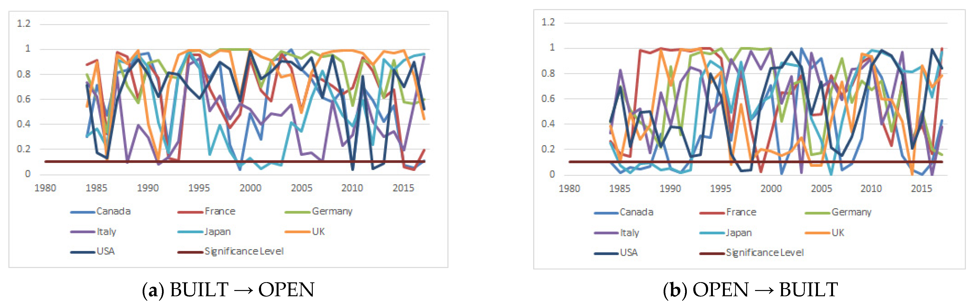
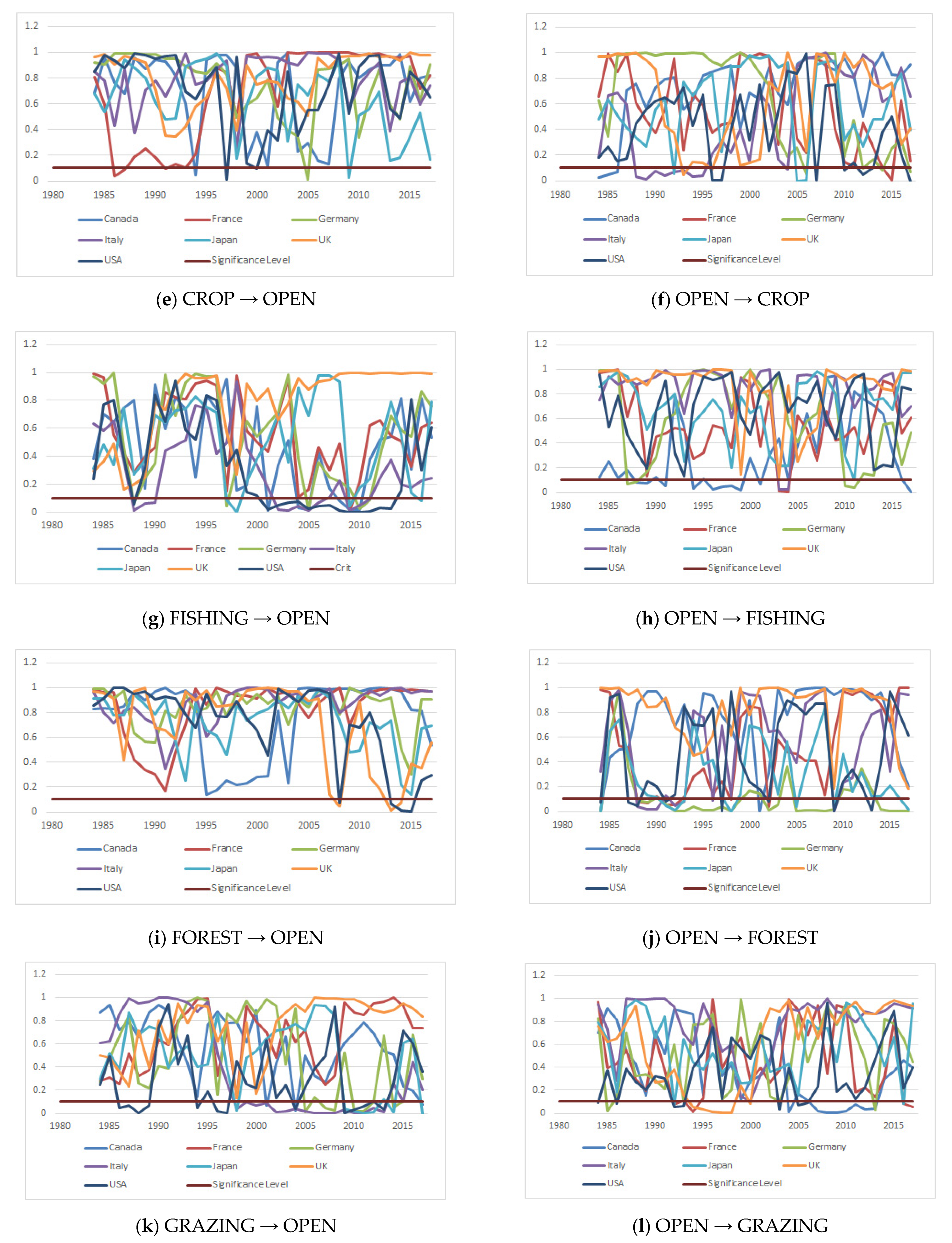
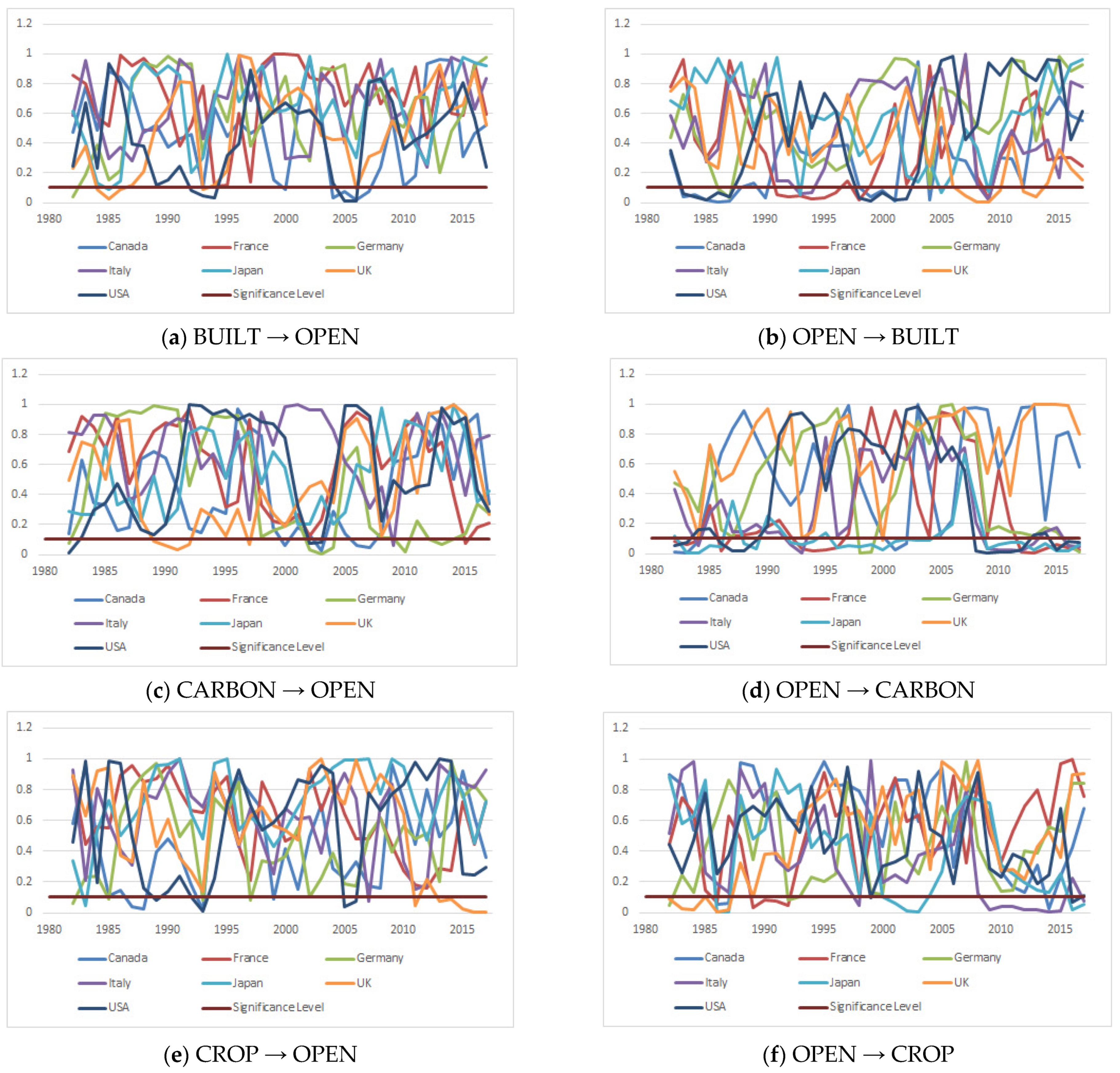
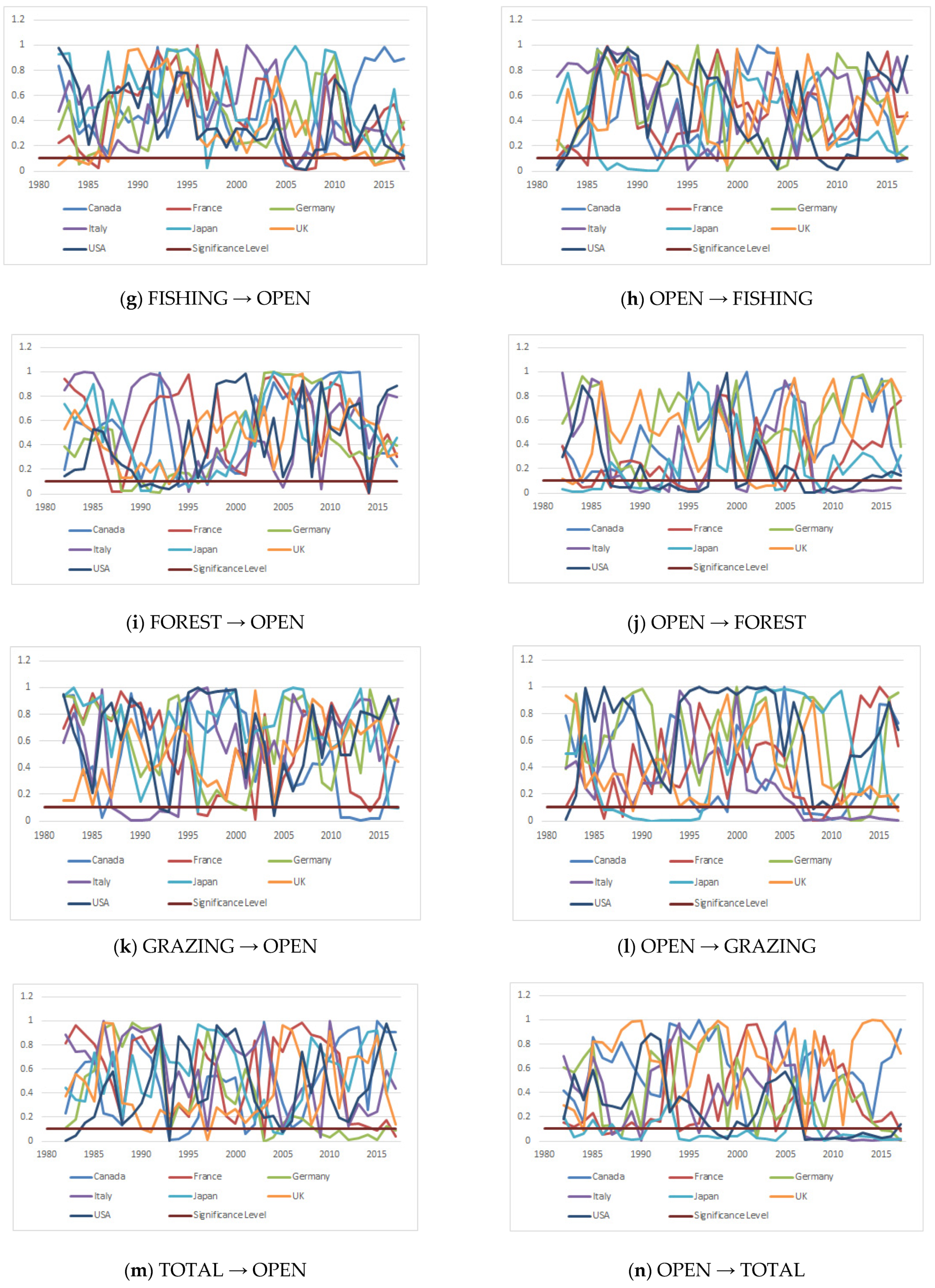
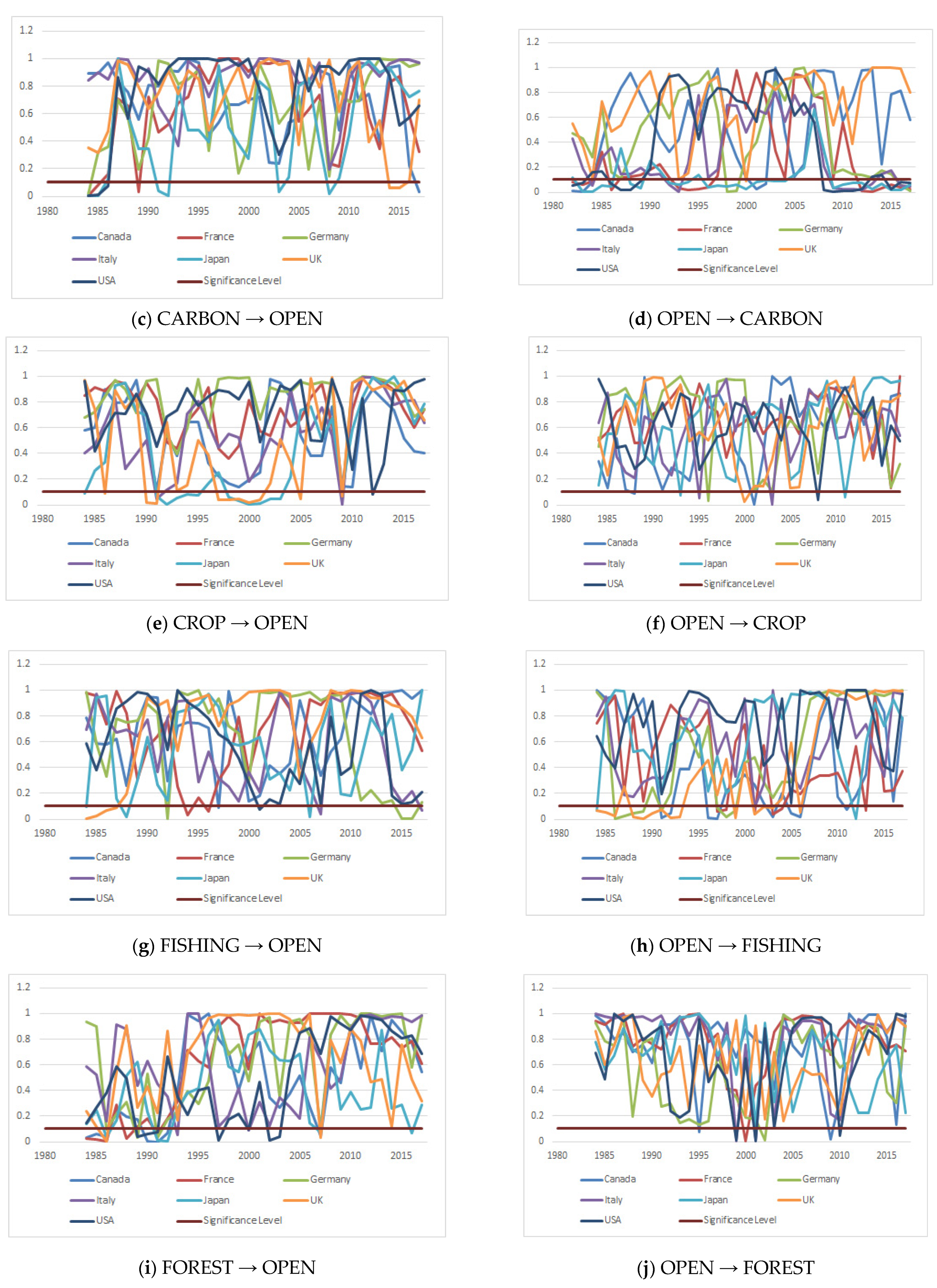
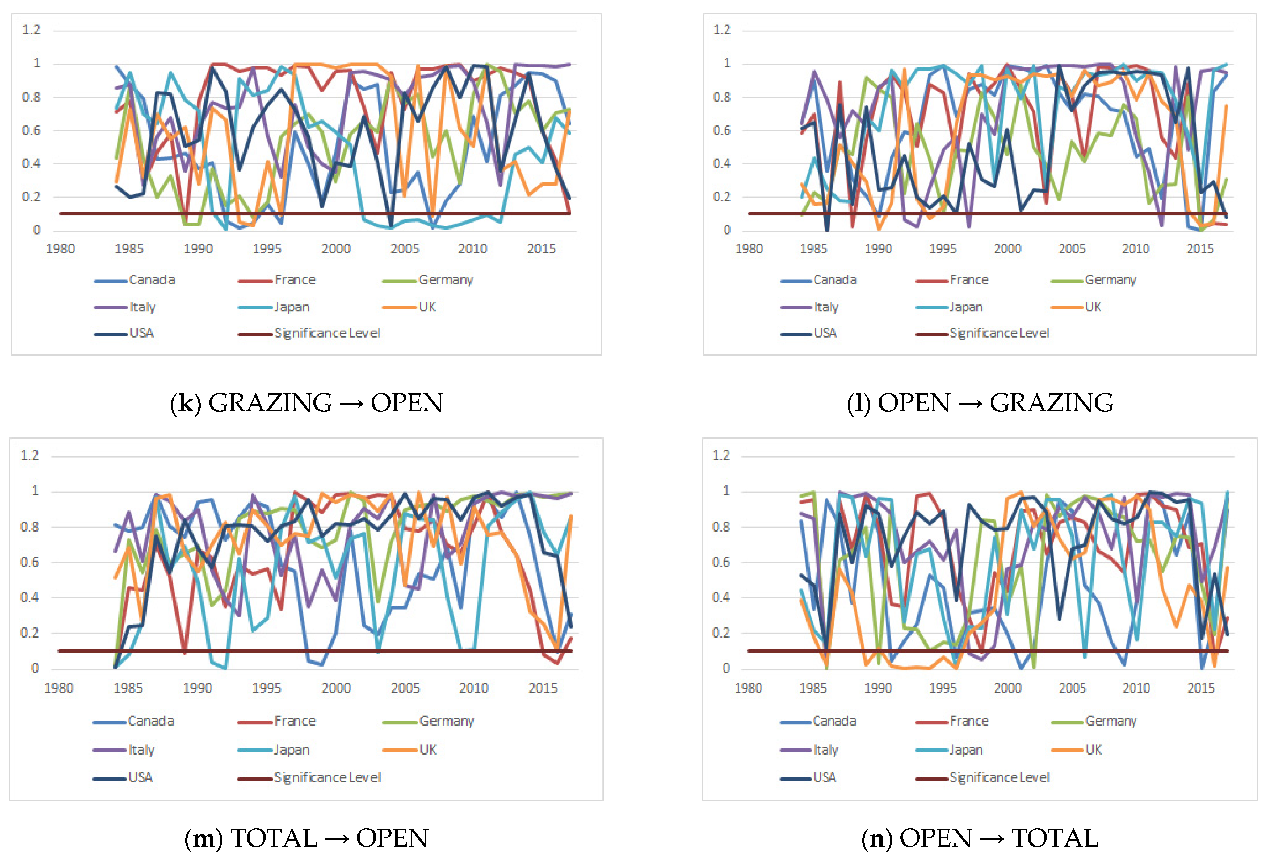
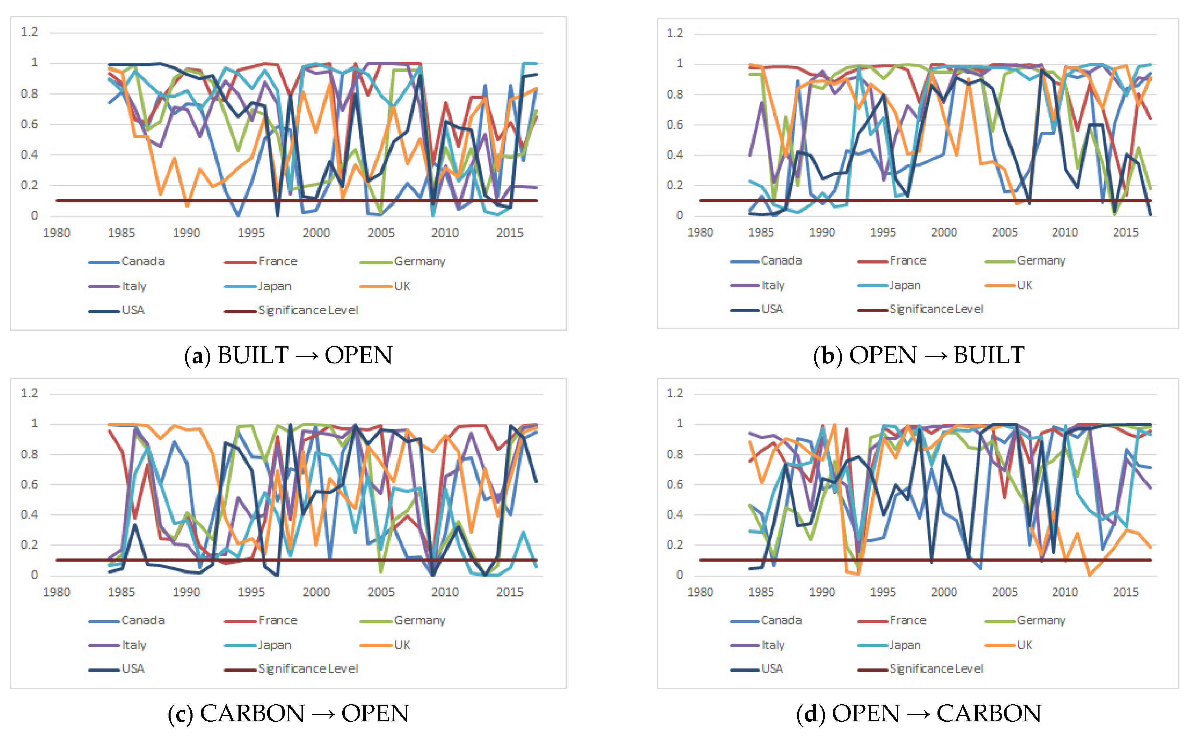
- In the OPEN → BUILT causality relationship in Annex 2, where the results of dynamic symmetric causality analysis are included, a strong causality relationship is observed in almost all countries in 2009. This date, on the other hand, can be interpreted as the effect of both the collapse experienced in all world economies after the 2008 global crisis and the recovery efforts afterward. Again, it is seen that there was a strong causality relationship in all countries in 1986 between many variables, especially the OPEN → CROP causality relationship. The year 1986 was the year of the Chernobyl nuclear power plant explosion, which is seen as the biggest environmental disaster in the history of the world.
- ➢
- If one examines Annex 3, which includes the results of dynamic asymmetric causality analysis between positive shocks, there is a strong causal relationship between many variables in Canada in 2015. As the reason for this, it is thought that the federal elections held in Canada in 2015 will have significant effects in terms of both environmental and economic policies.
- ➢
- Looking at Annex 4, which includes the results of dynamic asymmetric causality analysis between negative shocks, the year 2014 in Germany draws attention due to the strong causality relationship between many variables. The year 2014 is the period when an armament budget of 100 billion Euros was accepted for the modernization of the army in Germany after the Crimean conflict between Ukraine and Russia. It is estimated that this budget will create effects between variables, especially in the economic field.
5. Conclusions
- From CARBON to OPEN in Canada (14.874 test statistics value at 1% significance level) and Germany (16.436 test statistics value at 5% significance).
- From OPEN to CARBON in Italy (4.451 test statistics value at 1% significance level) and Japan (4.785 test statistics value at 5% significance).
- From OPEN to CROP for Germany (8.379 test statistics value at 10% significance level) and the UK (13.918 test statistics value at 5% significance level).
- From OPEN to FISHING for the UK (2.681 test statistics value at 5% significance level).
- From FOREST to OPEN for Japan (3.008 test statistics value at 5% significance level).
- From OPEN to FOREST for France (8.194 test statistics value at 1% significance level), Germany (10.694 test statistics value at 1% significance level), the UK (4.550 test statistics value at 1% significance level), and the USA (15.705 test statistics value at 5% significance level).
- From GRAZING to OPEN for only Germany (19.706 test statistics value at 1% significance level).
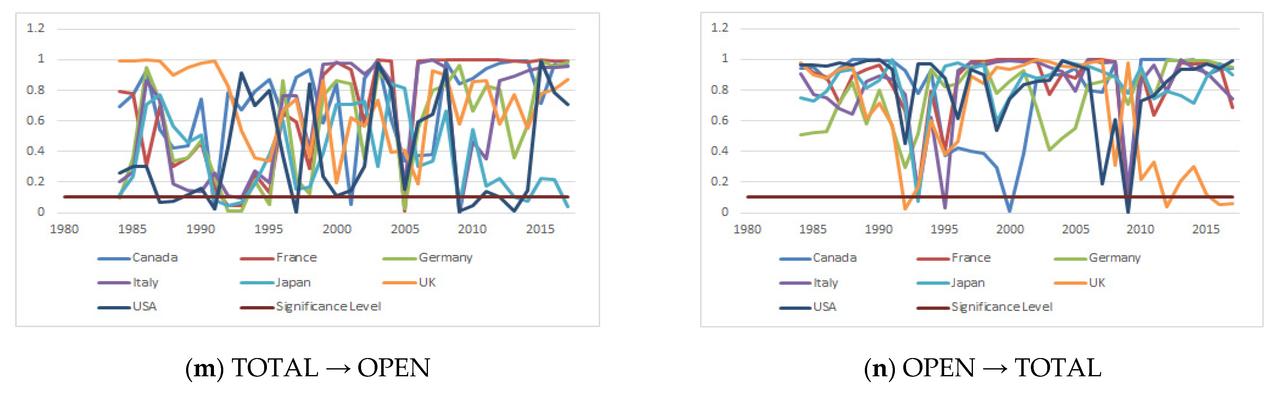
- From TOTAL to OPEN for Canada (3.001 test statistics value at 10% significance level) and Germany (11.595 test statistics value at 1% significance level).
- From OPEN to TOTAL for France (8.483 test statistics value at 10% significance level), Italy (3.649 test statistics value at 1% significance level), and Japan (25.416 test statistics value at 1% significance level).
- For positive shocks, we found a one-way causality that runs from GRAZING to OPEN for Canada (3.742 test statistics value at 1% significance level) and the UK (7.640 test statistics value at 10% significance level).
- For negative shocks, we conclude that there is a unidirectional causality that runs from FISHING to OPEN for Italy (33.333 test statistics value at 10% significance level), and from FOREST to OPEN for Japan (21.487 test statistics value at 10% significance level).
Author Contributions
Funding
Institutional Review Board Statement
Informed Consent Statement
Data Availability Statement
Conflicts of Interest
Appendix A. Results of Symmetric and Asymmetric Panel Causality Tests

| H0: BUILT ↛ OPEN | Symmetric Causality | Positive Shocks | Negative Shocks | |||
|---|---|---|---|---|---|---|
| Test Stat. | Bootstrap p-Value | Test Stat. | Bootstrap p-Value | Test Stat. | Bootstrap p-Value | |
| Canada | 0.038 | 0.777 | 0.889 | 0.946 | 5.941 | 0.841 |
| France | 2.394 | 0.957 | 2.594 | 0.994 | 4.056 | 1.000 |
| Germany | 10.918 | 0.332 | 19.490 | 0.275 | 6.148 | 0.965 |
| Italy | 0.226 | 0.528 | 6.065 | 0.870 | 3.423 | 1.000 |
| Japan | 0.014 | 0.876 | 0.752 | 0.986 | 0.085 | 0.999 |
| UK | 0.230 | 0.539 | 0.897 | 0.998 | 5.769 | 0.963 |
| USA | 6.045 | 0.129 | 3.710 | 0.850 | 1.464 | 0.906 |
| H0: OPEN ↛ BUILT | ||||||
| Canada | 1.038 | 0.892 | 4.206 | 0.365 | 0.048 | 0.998 |
| France | 1.677 | 0.847 | 6.271 | 0.785 | 0.984 | 0.999 |
| Germany | 6.134 | 0.972 | 6.572 | 0.975 | 2.538 | 0.989 |
| Italy | 0.680 | 0.215 | 0.299 | 0.957 | 2.455 | 0.993 |
| Japan | 0.067 | 0.949 | 1.776 | 0.945 | 2.997 | 0.926 |
| UK | 0.029 | 0.886 | 8.777 | 0.743 | 2.011 | 0.993 |
| USA | 20.158 | 0.286 | 0.927 | 0.900 | 3.919 | 0.423 |
| H0: CARBON ↛ OPEN | ||||||
| Canada | 14.874 * | 0.000 | 1.238 | 0.336 | 2.457 | 0.944 |
| France | 3.133 | 0.608 | 1.314 | 0.940 | 3.239 | 0.998 |
| Germany | 16.436 ** | 0.025 | 0.254 | 0.826 | 2.539 | 1.000 |
| Italy | 0.041 | 0.804 | 0.315 | 0.999 | 2.890 | 0.971 |
| Japan | 1.652 | 0.223 | 0.054 | 0.960 | 13.135 | 0.964 |
| UK | 0.080 | 0.744 | 4.292 | 0.734 | 1.483 | 1.000 |
| USA | 0.000 | 0.993 | 0.139 | 0.996 | 11.313 | 0.985 |
| H0: OPEN ↛ CARBON | ||||||
| Canada | 0.031 | 0.729 | 3.980 | 0.169 | 0.472 | 0.997 |
| France | 5.022 | 0.290 | 0.808 | 0.999 | 2.220 | 0.725 |
| Germany | 1.042 | 0.991 | 7.225 | 0.922 | 4.887 | 0.933 |
| Italy | 4.451 * | 0.007 | 3.487 | 0.949 | 1.337 | 0.978 |
| Japan | 4.785 ** | 0.013 | 3.827 | 0.423 | 0.051 | 1.000 |
| UK | 2.329 | 0.877 | 1.120 | 0.903 | 0.203 | 0.999 |
| USA | 14.974 | 0.102 | 2.054 | 0.979 | 4.398 | 0.995 |
| H0: CROP ↛ OPEN | ||||||
| Canada | 0.216 | 0.597 | 0.685 | 0.926 | 1.370 | 0.997 |
| France | 0.061 | 0.814 | 2.386 | 0.948 | 11.483 | 0.932 |
| Germany | 0.017 | 0.901 | 12.899 | 0.526 | 7.082 | 0.963 |
| Italy | 1.411 | 0.755 | 4.093 | 0.726 | 3.350 | 0.993 |
| Japan | 0.539 | 1.000 | 0.061 | 0.899 | 9.460 | 0.552 |
| UK | 0.082 | 0.895 | 3.093 | 0.857 | 4.296 | 0.999 |
| USA | 2.839 | 0.260 | 1.916 | 0.726 | 0.030 | 0.975 |
| H0: OPEN ↛ CROP | ||||||
| Canada | 0.015 | 0.911 | 3.238 | 0.590 | 2.685 | 0.930 |
| France | 0.027 | 0.883 | 10.965 | 0.832 | 3.562 | 0.848 |
| Germany | 8.379 *** | 0.054 | 9.166 | 0.934 | 3.651 | 0.931 |
| Italy | 2.164 | 0.426 | 0.059 | 0.983 | 10.648 | 0.639 |
| Japan | 9.127 | 0.909 | 0.579 | 0.697 | 0.136 | 0.677 |
| UK | 13.918 ** | 0.047 | 6.342 | 0.373 | 5.367 | 0.998 |
| USA | 1.242 | 0.317 | 0.262 | 0.783 | 0.461 | 0.479 |
| H0: FISHING ↛ OPEN | ||||||
| Canada | 0.170 | 0.918 | 0.009 | 0.985 | 5.061 | 0.922 |
| France | 2.066 | 0.384 | 0.273 | 0.985 | 16.961 | 0.694 |
| Germany | 1.482 | 0.837 | 3.190 | 0.932 | 8.921 | 0.811 |
| Italy | 0.904 | 0.182 | 2.147 | 0.668 | 33.333 *** | 0.093 |
| Japan | 0.002 | 0.972 | 0.068 | 0.820 | 12.134 | 0.775 |
| UK | 0.016 | 0.842 | 5.236 | 0.602 | 5.640 | 0.997 |
| USA | 0.032 | 0.993 | 0.005 | 0.986 | 3.009 | 0.886 |
| H0: OPEN ↛ FISHING | ||||||
| Canada | 0.001 | 0.999 | 5.017 | 0.776 | 0.196 | 0.937 |
| France | 0.792 | 0.961 | 9.463 | 0.739 | 1.940 | 0.949 |
| Germany | 0.718 | 0.894 | 2.640 | 1.000 | 3.403 | 0.554 |
| Italy | 0.313 | 0.780 | 3.859 | 0.628 | 0.035 | 0.997 |
| Japan | 2.375 | 0.773 | 1.010 | 0.954 | 0.241 | 0.858 |
| UK | 2.681 ** | 0.015 | 2.610 | 0.908 | 0.332 | 0.999 |
| USA | 1.076 | 0.981 | 1.879 | 0.973 | 0.101 | 0.997 |
| H0: FOREST ↛ OPEN | ||||||
| Canada | 1.129 | 0.285 | 0.293 | 0.645 | 3.940 | 1.000 |
| France | 0.999 | 0.518 | 0.034 | 1.000 | 4.252 | 1.000 |
| Germany | 0.836 | 0.317 | 2.074 | 0.999 | 22.297 | 0.533 |
| Italy | 0.028 | 0.948 | 0.021 | 1.000 | 5.619 | 0.922 |
| Japan | 3.008 ** | 0.014 | 0.116 | 0.962 | 21.487 *** | 0.061 |
| UK | 1.005 | 0.450 | 0.265 | 1.000 | 1.109 | 1.000 |
| USA | 0.111 | 0.568 | 0.046 | 0.997 | 20.257 | 0.815 |
| H0: OPEN ↛ FOREST | ||||||
| Canada | 10.488 | 0.109 | 4.949 | 0.646 | 0.003 | 1.000 |
| France | 8.194 * | 0.001 | 0.494 | 0.999 | 0.276 | 1.000 |
| Germany | 10.694 * | 0.006 | 2.079 | 1.000 | 5.239 | 0.960 |
| Italy | 0.009 | 1.000 | 0.170 | 1.000 | 1.036 | 1.000 |
| Japan | 0.880 | 0.569 | 6.115 | 0.571 | 0.635 | 0.974 |
| UK | 4.550 * | 0.003 | 0.616 | 0.979 | 1.204 | 1.000 |
| USA | 15.705 ** | 0.021 | 1.137 | 0.853 | 0.342 | 0.997 |
| H0: GRAZING ↛ OPEN | ||||||
| Canada | 0.589 | 0.799 | 3.742 * | 0.003 | 14.973 | 0.732 |
| France | 10.334 | 0.724 | 0.001 | 0.997 | 10.545 | 0.980 |
| Germany | 19.706 * | 0.002 | 3.641 | 0.598 | 1.816 | 0.985 |
| Italy | 2.014 | 0.928 | 0.881 | 0.984 | 8.449 | 0.941 |
| Japan | 0.002 | 0.985 | 0.409 | 0.358 | 8.777 | 0.469 |
| UK | 0.068 | 0.846 | 7.640 *** | 0.093 | 5.800 | 0.984 |
| USA | 0.216 | 1.000 | 4.465 | 0.161 | 19.451 | 0.245 |
| H0: OPEN ↛ GRAZING | ||||||
| Canada | 0.324 | 0.999 | 2.542 | 0.455 | 6.433 | 0.411 |
| France | 5.870 | 0.683 | 1.584 | 0.985 | 8.819 | 0.633 |
| Germany | 0.021 | 0.981 | 21.641 | 0.258 | 2.575 | 0.721 |
| Italy | 3.535 | 0.414 | 2.444 | 0.998 | 0.965 | 0.993 |
| Japan | 0.007 | 1.000 | 10.318 | 0.540 | 1.418 | 0.853 |
| UK | 0.704 | 0.497 | 0.090 | 0.788 | 6.319 | 0.940 |
| USA | 4.358 | 1.000 | 2.410 | 0.933 | 1.466 | 0.457 |
| H0: TOTAL ↛ OPEN | ||||||
| Canada | 3.001 *** | 0.051 | 0.015 | 0.976 | 4.440 | 0.997 |
| France | 1.381 | 0.476 | 1.268 | 0.949 | 9.233 | 0.998 |
| Germany | 11.595 * | 0.009 | 0.859 | 0.999 | 6.524 | 1.000 |
| Italy | 0.008 | 0.894 | 0.351 | 0.998 | 3.711 | 0.980 |
| Japan | 3.426 | 0.176 | 0.072 | 0.910 | 16.839 | 0.889 |
| UK | 0.166 | 0.745 | 2.919 | 0.885 | 3.304 | 1.000 |
| USA | 0.837 | 0.339 | 1.375 | 0.882 | 8.307 | 0.991 |
| H0: OPEN ↛ TOTAL | ||||||
| Canada | 1.943 | 0.863 | 5.193 | 0.465 | 2.445 | 0.941 |
| France | 8.483 *** | 0.058 | 0.844 | 0.966 | 0.124 | 1.000 |
| Germany | 0.844 | 0.950 | 11.598 | 0.939 | 4.109 | 0.985 |
| Italy | 3.649 * | 0.000 | 1.910 | 0.980 | 1.626 | 0.995 |
| Japan | 25.416 * | 0.000 | 5.133 | 0.270 | 0.003 | 1.000 |
| UK | 3.773 | 0.756 | 1.000 | 0.963 | 0.399 | 1.000 |
| USA | 11.960 | 0.175 | 1.566 | 0.967 | 0.038 | 0.998 |
Appendix B. Results of Dynamic Symmetric Panel Causality Test
| Direction of Causality | Canada | France | Germany | Italy | Japan | UK | USA |
|---|---|---|---|---|---|---|---|
| BUILT → OPEN | 2000-2004-2005-2006-2007 | - | 1982 | - | 1985 | 1984-1985-1986-1993-2006 | 1992-1993-1994-2005-2006 |
| OPEN → BUILT | 1983-1984-1985-1986-1987-1990-1999-2000-2001-2004-2009 | 1991-1992-1993-1994-1995-1996-1998-2009 | 1986-1987-2004 | 1993-1994-2009 | 1993-2005-2009 | 2007-2008-2009-2010-2012-2013 | 1983-1984-1985-1986-1987-1998-1999-2000-2001-2002 |
| CARBON → OPEN | 2000-2003-2006-2007 | 2015 | 1982-2002-2003-2004-2010-2013 | 2009 | - | 1989-1990-1991-1992-1997 | 1982-2002-2003 |
| OPEN → CARBON | 1982-1983-1984-2001-2002 | 1982-1983-1984-1986-1993-1994-1995-1996-2012-2013-2014-2015-2016-2017 | 1998-1999-2016-2017 | 1984-1992-1993-2009-2010-2011-2012-2013-2016-2017 | 1983-1984-1985-1986-1988-1989-1992-1993-1994-1996-1997-1998-1999-2000-2001-2002-2003-2004-2009-2010-2011-2012-2013-2014-2015-2016-2017 | 2000 | 1982-1983-1986-1987-1988-1989-2008-2009-2010-2011-2012-2015-2016-2017 |
| CROP → OPEN | 1987-1988-1993-1999 | - | 1982-1985-1993-1997 | 2007 | 1983 | 2011-2013-2014-2015-2016-2017 | 1989-1993-2005-2006 |
| OPEN → CROP | 1986-1987-2014 | 1986-1989-1990-1991-1992 | 1982-1992 | 1998-2009-2010-2011-2012-2013-2014-2015-2017 | 1986-1987-2001-2002-2003-2016-2017 | 1982-1983-1984-1986-1987 | 1999-2016 |
| FISHING → OPEN | 2005-2006 | 1985-1986-2005-2006-2007-2008 | 1984-2014 | 1987-2006-2017 | 1997-2017 | 1982-1984-1985-1987-2008-2011-2014-2015-2016 | 2006-2007 |
| OPEN → FISHING | 1982-1992-2016 | 1985 | 1999-2004-2005-2017 | 1995-1998-2006 | 1987-1988-1989-1990-1991-1992 | 1999 | 1982-2004-2009-2010 |
| Forest → OPEN | 1994-2014 | 1987-1988-2014 | 1988-1989-1991-1992-1996 | 1995-1997-2005-2009 | 1990-1991-1993-1995-1997 | 1993 | 1990-1991-1992-1993-1994-2014 |
| OPEN → Forest | 1984-1994 | 1984-1985-1987-1994-1995-1996-2005-2008-2009 | 1990-2001 | 1989-1990-1991-1992-1993-1996-2000-2001-2008-2009-2010-2011-2012-2013-2014-2015-2016-2017 | 1982-1983-1984-1985-1986-1989-1990-1991-1992-2004-2005-2009 | 1983-2001-2002-2003-2004 | 1987-1988-1989-1991-1992-1993-1994-1995-1996-1997-2000-2001-2007-2008-2009-2010-2011-2012 |
| GRAZING → OPEN | 1986-2011-2012-2013-2014-2015 | 1996-1997-2002-2004-2014 | 2001 | 1988-1989-1990-1991-1992-1993-1994 | 1996-2017 | - | 1992-1993-2004 |
| OPEN → GRAZING | 1996-1999-2007-2008-2009-2010-2011 | 1986-1988-2008-2009 | 2012-2013-2014 | 2007-2008-2009-2010-2011-2012-2013-2014-2015-2016-2017 | 1986-1987-1988-1989-1990-1991-1992-1993-1994-1995-1996 | 1989-2017 | 1982-2008-2010 |
| TOTAL → OPEN | 1993-1994-1995-2001 | 2003-2015-2017 | 1993-2003-2004-2009-2010-2011-2012-2013-2014-2015-2017 | 1997-2009 | 2004-2005 | 1991-1997 | 1982-1983-1993-2005 |
| OPEN → TOTAL | 2001-2002 | 1986-1987-1988-1990-1994-2004-2007-2017 | 1988-1999-2002-2009-2015-2016-2017 | 1987-1988-1990-1996-2007-2008-2009-2011-2012-2013-2014-2015-2016-2017 | 1983-1984-1986-1988-1989-1989-1990-1994-1995-1996-1997-1998-1999-2000-2001-2002-2003-2004-2005-2009-2010-2011-2012-2013-2014-2015-2016-2017 | 1984-2007 | 1998-1999-2007-2008-2009-2010-2011-2012-2013-2014-2015-2016 |
Appendix C. Results of Dynamic Asymmetric Panel Causality Test between Positive Shocks
| Direction of Causality | Canada | France | Germany | Italy | Japan | UK | USA |
|---|---|---|---|---|---|---|---|
| BUILT → OPEN | 1999-2010-2015-2016 | 2015-2016 | - | 1988-1991 | 1999-2001-2002-2003 | - | 2010-2012-2013 |
| OPEN → BUILT | 1985-1986-1987-1988-1990-1991-2001-2007-2008-2014-2015-2016 | 1999 | - | 2003-2016 | 1985-1986-1987-1988- 1989-1990-1991-1992-2006 | 1996-2004-2005-2014 | 1997-1998 |
| CARBON → OPEN | 2017 | 1984-1985-1989 | 1984 | - | 1984-1985-1991- 1992-2003-2008 | 2014-2015 | 1984-1985-1986 |
| OPEN → CARBON | 1984-2000-2015 | - | 1996-1997-1998-2004-2014 | 1999 | 1985-2000-2010 | 1988-1989-1990-1991-1992-1993-1994-1996 | - |
| CROP → OPEN | - | - | 2009 | 1991-2009 | 1984-1991-1992- 1993-1994-1995- 1998-1999-2000- 2001-2002-2003 | 1986-1990-1991-1997-1998-1999-2000-2001-2005-2009 | 2012 |
| OPEN → CROP | 1988-2001 | - | 1996 | 1995-2003 | 1993-2011 | 2000 | 2008 |
| FISHING → OPEN | 1997 | 1994-1996 | 1992-2015-2016 | 2007-2017 | 1984-1988-2006 | 1984-1985-1986-1987 | 2001 |
| OPEN → FISHING | 1991-1992-1996-1997-2003-2005-2006-2011 | 1997-1998-2001-2003-2004-2013 | 1986-1987-1988-1989-1991-1997-1998-1999 | 2001 | 1984-2012 | 1984-1985-1986-1988-1989-1990-1991-1992-1993-1999-2001-2002-2003-2006 | - |
| FOREST → OPEN | 1984-1985-1986-1990-1991-1992-2007 | 1984-1985-1986-1988-1991 | 1986-1989-1991-2007 | 1993-2000 | 1986-1991-1992-2007-2016 | 1986-2007 | 1989-1990-1991-1997-2000-2002-2003 |
| OPEN → FOREST | 1995-2009 | 2000 | 2002 | 1999-2001 | - | - | 1999-2001-2010 |
| GRAZING → OPEN | 1992-1993-1994-1996-2007 | 1989 | 1989-1990-1994 | - | 1992-2002-2003-2004- 2005-2006-2007- 2008-2009-2010-2011-2012 | 1993-1994-1996-2007 | 2004 |
| OPEN → GRAZING | 1990-2014-2015 | 1986-1988-2015-2016-2017 | 1984-2015-2016 | 1992-1993-1997-2012 | - | 1990-1994-2015-2016 | 1986-2017 |
| TOTAL → OPEN | 1998-1999-2016 | 1984-1989-2015-2016 | 1984 | - | 1984-1985-1991- 1992-2003 | - | 1984 |
| OPEN → TOTAL | 1991-1996-2001-2009-2015 | 1986-1998-2016 | 1986-1990-2002 | 1986-1997-1998 | 1996-2006 | 1986-1989-1991-1992-1993-1994-1995-1996-2016 | - |
Appendix D. Results of Dynamic Asymmetric Panel Causality Test between Negative Shocks
| Direction of Causality | Canada | France | Germany | Italy | Japan | UK | USA |
|---|---|---|---|---|---|---|---|
| BUILT → OPEN | 1994-1999-2000-2004-2005-2006-2011-2012 | - | 2005 | 2009-2011-2014 | 2009- 2013- 2014- 2015 | 1990 | 1997-2009-2014-2015 |
| OPEN → BUILT | 1984-1986-1987-1990-2013 | - | 1986-2014 | - | 1986- 1987- 1988- 1989- 1991- 1992 | 2006 | 1984-1985-1986-1987-2007-2014-2017 |
| CARBON → OPEN | 1991-2009 | 1993-1994 | 1984-2005-2013-2014 | 2009 | 1984- 1985- 1992- 2012- 2013- 2014- 2015- 2017 | 1984-1985-1987-1988-1989-1990-1991-1992-1996-1997-2009-2013 | - |
| OPEN → CARBON | 1986-2003 | 1993 | 1993 | 2008 | - | 1992-1993-2010-2012-2013 | 1984-1985-1999 |
| CROP → OPEN | 1994 | 1986-1987-1991 | 2005 | - | 2009 | - | 1997-2000 |
| OPEN → CROP | 1984-1985-1986 | 2015 | 2006-2012-2014-2017 | 1988-1989-1990-1991-1992-1993-1994-1995-2004 | 1992- 2005-2006 | 1993-1996 | 1996-1997-2007-2010-2012-2017 |
| FISHING → OPEN | 2001-2004-2005-2008-2009-2010 | 2009 | 1988-1997-2005-2010-2011 | 1988-1989-1990-2002-2003-2004-2005-2006-2009-2010-2011 | 1997- 1998- 2009-2016 | 1988-2001-2002-2003-2004-2005-2006-2007-2008-2009-2010-2011-2012-2013 | - |
| OPEN → FISHING | 1988-1989-1991-1994-1996-1997-1998-1999-2001-2017 | 2003-2004 | 1987-1988-2010-2011 | - | - | - | - |
| FOREST → OPEN | - | - | - | - | - | 2008-2013-2014 | 2008-2013-2014-2015 |
| OPEN → FOREST | 1984-2001 | 1988-1989-1991-1992-1998-2002 | 1984-1988-1989-1991-1992-1993-1994-1995-1996-1997-1998-1999-2002-2003-2005-2006-2007-2008-2009-2014-2015-2016-2017 | 1988-1989-1990-1992-1993-1996-2009 | 1984-1991- 1992-1993- 1998- 2005- 2009- 2017 | - | 1984-1987-1988-1991-1997-2002-2009-2013 |
| GRAZING → OPEN | 2001-2004-2017 | - | 2005-2007-2008-2010-2011-2012-2014 | 1998-1999-2000-2001-2002-2003-2005-2006-2007-2008-2009-2010-2011-2012-2013 | 1998- 2009- 2010- 2011- 2012- 2014- 2017 | - | 1986-1987-1988-1989-1994-1996-1997-2004-2009-2010-2011-2013 |
| OPEN → GRAZING | 2004-2007-2008-2009-2010-2011-2012-2013 | 1992-1994-2016-2017 | 1985-2013 | - | 1992-2016 | 1994-1995-1996-1997-1998-2000 | 1984-1986-1992-1993-2003-2005-2006 |
| TOTAL → OPEN | 1991-2001 | 1992-1993-2005 | 1984-1992-1993-1995-2005 | 1993-2009 | 1991- 1992- 1993- 2009- 2014- 2017 | - | 1987-1988-1991-1997-2009-2010-2013 |
| OPEN → TOTAL | 2000 | 2009 | - | 1995 | 1993 | 1992-2012-2016-2017 | 2009 |
References
- Moran, D.D.; Lenzen, M.; Kanemoto, K.; Geschke, A. Does ecologically unequal exchange occur? Ecol. Econ. 2013, 89, 177–186. [Google Scholar] [CrossRef]
- Wackernagel, M.; Rees, W. Our Ecological Footprint: Reducing Human Impact on the Earth; New Society Publishers: Gabriola Island, BC, Canada, 1996. [Google Scholar]
- Aitken, A.C. On Least-squares and Linear Combinations of Observations. In Proceedings of the Royal Society of Edinburgh; Cambridge University Press: Cambridge, UK, 1936; Volume 55, pp. 42–48. [Google Scholar]
- Andersson, J.O.; ve Lindroth, M. Ecologically unsustainable trade. Ecol. Econ. 2001, 37, 113–122. [Google Scholar] [CrossRef]
- Dam, T.A.; Pasche, M.; Werlich, N. Trade patterns and the ecological footprint a theory-based empirical approach. In Jena Economic Research Papers; No. 2017-005; Friedrich Schiller University Jena: Jena, Germany, 2017. [Google Scholar]
- Destek, M.A.; Sarkodie, S.A. Investigation of Environmental Kuznets Curve for Ecological Footprint: The Role of Energy And Financial Development. Sci. Total Environ. 2019, 650, 2483–2489. [Google Scholar] [CrossRef]
- Granger, C.W.; Yoon, G. Hidden Cointegration; Economics Working Paper (2002-02); University of California: San Diego, CA, USA, 2002. [Google Scholar]
- Proops, J.L.R.; Atkinson, G.; Schlotheim, B.F.V.; Simon, S. Analysıs International Trade and The Sustainability Footprint: A Practical Criterion For İts Assessment. Ecol. Econ. 1999, 28, 75–97. [Google Scholar] [CrossRef]
- Rehman, A.; Radulescu, M.; Ma, H.; Dagar, V.; Hussain, I.; Khan, M.K. The Impact of Globalization, Energy Use, and Trade on Ecological Footprint in Pakistan: Does Environmental Sustainability Exist? Energies 2021, 14, 5234. [Google Scholar] [CrossRef]
- Udemba, E.N. Ascertainment of Ecological Footprint and Environmental Kuznets in China. In Assessment of Ecological Footprints. Environmental Footprints and Eco-Design of Products and Processes; Muthu, S.S., Ed.; Springer: Singapore, 2021. [Google Scholar] [CrossRef]
- Phillips, P.C.; Shi, S.; Yu, J. Testing for multiple bubbles: Historical episodes of exuberance and collapse in the S&P 500. Int. Econ. Rev. 2015, 56, 1043–1078. [Google Scholar]
- Gao, J.; Tian, M. Analysis of over-consumption of natural resources and the ecological trade deficit in Chin abased on ecological footprints. Ecol. Indic. 2016, 61, 899–904. [Google Scholar] [CrossRef]
- Choi, E.; Heshmati, A.; ve Cho, Y. An Empirical Study of the Relationship between CO2 Emissions, Economic Growth and Openness; IZA Discussion Paper Series 5304; IZA: Bonn, Germany, 2010. [Google Scholar]
- Al-Mulali, U.; Weng-Wai, C.; Low, S.T.; Mohammed, A.H. Investigating the environmental kuznets curve (EKC) hypothesis by utilizing the ecological footprint as an indicator of environmental degradation. Ecol. Indic. 2014, 48, 315–323. [Google Scholar] [CrossRef]
- Ali, S.; Yusop, Z.; Meo, M.S. Asymmetric openness-environment nexus in most open OIC countries: New evidence from quantile-on-quantile (QQ) estimation. Environ. Sci. Pollut. Res. 2022, 29, 26352–26370. [Google Scholar] [CrossRef]
- Usman, M.; Kousar, R.; Yaseen, M.R.; Makhdum, M.S.A. An empirical nexus between economic growth, energy utilization, trade policy, and ecological footprint: A continent-wise comparison in upper-middle-income countries. Environ. Sci. Pollut. Res. 2020, 27, 38995–39018. [Google Scholar] [CrossRef]
- Ansari, M.A.; Ahmad, M.R.; Siddique, S.; Mansoor, K. An environment Kuznets curve for ecological footprint: Evidence from GCC countries. Carbon Manag. 2020, 11, 355–368. [Google Scholar] [CrossRef]
- Fotros, M.H.; Maaboudi, R. The Impact of Trade Openness on CO2 Emissions in Iran, 1971–2005. 2010. Available online: https://www.gtap.agecon.purdue.edu/resources/download/5112.pdf (accessed on 14 February 2022).
- Kónya, L. Exports and growth: Granger causality analysis on OECD countries with a panel data approach. Econ. Model. 2006, 23, 978–992. [Google Scholar] [CrossRef]
- Erdoğan, S.; Gedikli, A.; Kırca, M. A note on time-varying causality between natural gas consumption and economic growth in Turkey. Resour. Policy 2019, 64, 101504. [Google Scholar] [CrossRef]
- Jorgenson, A.K.; Rice, J. Structural dynamics of international trade and material consumption: A cross-national study of the ecological footprints of less-developed Countries. J. World Syst. 2005, 11, 57–77. [Google Scholar] [CrossRef] [Green Version]
- Ghita, S.I.; Saseanu, A.S.; Gogonea, R.M.; ve Huidumac-Petrescu, C.E. Perspectives of ecological footprint in european context under the ımpact of ınformation society and sustainable development. Sustainability 2018, 10, 3224. [Google Scholar] [CrossRef] [Green Version]
- Zellner, A. An efficient method of estimating seemingly unrelated regressions and tests for aggregation bias. J. Am. Stat. Assoc. 1962, 57, 348–368. [Google Scholar] [CrossRef]
- Granger, C.W. Investigating causal relations by econometric models and cross-spectral methods. Econom. J. Econom. Soc. 1969, 37, 424–438. [Google Scholar] [CrossRef]
- Hatemi-j, A. Asymmetric causality tests with an application. Empir. Econ. 2012, 43, 447–456. [Google Scholar] [CrossRef]
- Yilanci, V.; Aydin, M. Oil prices and stock prices: An asymmetric panel causality approach. J. Appl. Res. Financ. Econ. 2016, 2, 9–19. [Google Scholar]
- Dogan, E.; Ulucak, R.; Kocak, E.; Isik, C. The Use of Ecological Footprint in Estimating the Environmental Kuznets Curve Hypothesis for BRICST by Considering Cross-Section Dependence and Heterogeneity. Sci. Total Environ. 2020, 723, 138063. [Google Scholar] [CrossRef]
- Sim, N.; Zhou, H. Oil prices, US stock return, and the dependence between their quantiles. J. Bank. Financ. 2015, 55, 1–8. [Google Scholar] [CrossRef]
- Hervieux, M.-S.; Darné, O. Environmental Kuznets curve and ecological footprint: A time series analysis. Econ. Bull. 2015, 35, 814–826. [Google Scholar]
- Alam, S. Globalization, poverty and environmental degradation: Sustainable development in Pakistan. J. Sustain. Dev. 2010, 3, 103–114. [Google Scholar] [CrossRef] [Green Version]
- Saqib, M.; Benhmad, F. Does ecological footprint matter for the shape of the environmental Kuznets curve? Evidence from European countries. Environ. Sci. Pollut. Res. 2021, 28, 13634–13648. [Google Scholar] [CrossRef]
- Yilanci, V.; Pata, U.K.; Cutcu, I. Testing the Persistence of Shocks on Ecological Footprint and Sub-accounts: Evidence from the Big Ten Emerging Markets. Int. J. Environ. Res. 2022, 16, 10. [Google Scholar] [CrossRef]
- Moran, D.D.; Wackernagel, M.C.; Kitzes, J.A.; Heumann, B.W.; Phan, D.; Goldfinger, S.H. Trading spaces: Calculating embodied ecological footprints in international tradeusing a product land use matrix (PLUM). Ecol. Econ. 2009, 68, 1938–1951. [Google Scholar] [CrossRef]


| BUILT | |||||||||
|---|---|---|---|---|---|---|---|---|---|
| Countries | Mean | Median | Maximum | Minimum | Std. Dev. | Skewness | Kurtosis | Jarque-Bera | Probability |
| Canada | 0.062 | 0.061 | 0.098 | 0.037 | 0.015 | 0.379 | 2.297 | 2.137 | 0.343 |
| France | 0.134 | 0.143 | 0.166 | 0.081 | 0.024 | −0.659 | 2.165 | 4.872 | 0.088 *** |
| Germany | 0.109 | 0.106 | 0.144 | 0.073 | 0.020 | 0.002 | 1.772 | 3.017 | 0.221 |
| Italy | 0.048 | 0.047 | 0.056 | 0.037 | 0.005 | −0.111 | 2.115 | 1.663 | 0.435 |
| Japan | 0.065 | 0.064 | 0.078 | 0.054 | 0.007 | 0.075 | 1.799 | 2.933 | 0.231 |
| UK | 0.128 | 0.136 | 0.153 | 0.076 | 0.022 | −0.937 | 2.602 | 7.334 | 0.026 ** |
| USA | 0.057 | 0.057 | 0.078 | 0.038 | 0.011 | 0.019 | 1.900 | 2.424 | 0.298 |
| CARBON | |||||||||
| Countries | Mean | Median | Maximum | Minimum | Std. Dev. | Skewness | Kurtosis | Jarque-Bera | Probability |
| Canada | 5.217 | 5.340 | 6.035 | 4.270 | 0.446 | −0.267 | 2.150 | 2.014 | 0.365 |
| France | 3.139 | 3.078 | 3.980 | 2.611 | 0.338 | 0.619 | 2.664 | 3.291 | 0.193 |
| Germany | 4.192 | 4.115 | 5.414 | 3.176 | 0.639 | 0.077 | 1.739 | 3.227 | 0.199 |
| Italy | 2.947 | 2.838 | 3.730 | 2.383 | 0.403 | 0.426 | 2.016 | 3.391 | 0.183 |
| Japan | 3.423 | 3.536 | 3.894 | 2.713 | 0.318 | −0.674 | 2.393 | 4.372 | 0.112 |
| UK | 3.798 | 3.811 | 4.780 | 2.645 | 0.480 | −0.232 | 2.863 | 0.468 | 0.791 |
| USA | 7.116 | 7.253 | 8.335 | 5.742 | 0.667 | −0.511 | 2.562 | 2.471 | 0.291 |
| CROP | |||||||||
| Countries | Mean | Median | Maximum | Minimum | Std. Dev. | Skewness | Kurtosis | Jarque-Bera | Probability |
| Canada | 1.172 | 1.186 | 1.648 | 0.651 | 0.240 | −0.179 | 2.241 | 1.407 | 0.495 |
| France | 0.881 | 0.882 | 1.057 | 0.672 | 0.083 | −0.180 | 3.025 | 0.261 | 0.878 |
| Germany | 0.856 | 0.840 | 1.052 | 0.704 | 0.077 | 0.471 | 2.835 | 1.832 | 0.400 |
| Italy | 0.882 | 0.884 | 1.050 | 0.758 | 0.067 | 0.277 | 2.848 | 0.658 | 0.720 |
| Japan | 0.482 | 0.483 | 0.547 | 0.406 | 0.039 | −0.197 | 2.000 | 2.311 | 0.315 |
| UK | 0.732 | 0.736 | 0.814 | 0.630 | 0.045 | −0.292 | 2.270 | 1.746 | 0.418 |
| USA | 0.864 | 0.882 | 1.090 | 0.501 | 0.121 | −1.017 | 4.363 | 11.983 | 0.003 * |
| FISHING | |||||||||
| Countries | Mean | Median | Maximum | Minimum | Std. Dev. | Skewness | Kurtosis | Jarque-Bera | Probability |
| Canada | 0.334 | 0.240 | 0.645 | 0.124 | 0.183 | 0.403 | 1.567 | 5.410 | 0.067 *** |
| France | 0.216 | 0.210 | 0.256 | 0.170 | 0.025 | −0.005 | 1.745 | 3.148 | 0.207 |
| Germany | 0.097 | 0.071 | 0.223 | 0.046 | 0.053 | 1.125 | 3.030 | 10.127 | 0.006 * |
| Italy | 0.106 | 0.111 | 0.141 | 0.065 | 0.023 | −0.350 | 1.879 | 3.491 | 0.175 |
| Japan | 0.467 | 0.493 | 0.612 | 0.280 | 0.082 | −0.642 | 2.578 | 3.652 | 0.161 |
| UK | 0.184 | 0.164 | 0.412 | 0.079 | 0.095 | 0.987 | 3.057 | 7.806 | 0.020 |
| USA | 0.116 | 0.117 | 0.143 | 0.091 | 0.014 | −0.001 | 1.963 | 2.152 | 0.341 |
| FOREST | |||||||||
| Countries | Mean | Median | Maximum | Minimum | Std. Dev. | Skewness | Kurtosis | Jarque-Bera | Probability |
| Canada | 1.673 | 1.673 | 2.365 | 0.858 | 0.397 | 0.025 | 1.961 | 2.165 | 0.339 |
| France | 0.638 | 0.609 | 0.839 | 0.510 | 0.087 | 0.498 | 2.097 | 3.611 | 0.164 |
| Germany | 0.558 | 0.545 | 1.025 | 0.372 | 0.091 | 2.731 | 15.885 | 391.720 | 0.000 * |
| Italy | 0.422 | 0.439 | 0.574 | 0.230 | 0.095 | −0.096 | 1.870 | 2.626 | 0.269 |
| Japan | 0.412 | 0.447 | 0.661 | 0.223 | 0.125 | 0.022 | 1.938 | 2.258 | 0.323 |
| UK | 0.509 | 0.505 | 0.610 | 0.386 | 0.060 | 0.062 | 1.874 | 2.568 | 0.277 |
| USA | 1.163 | 1.238 | 1.423 | 0.735 | 0.193 | −0.988 | 2.618 | 8.094 | 0.017 ** |
| GRAZING | |||||||||
| Countries | Mean | Median | Maximum | Minimum | Std. Dev. | Skewness | Kurtosis | Jarque-Bera | Probability |
| Canada | 0.499 | 0.490 | 0.771 | 0.313 | 0.142 | 0.605 | 2.267 | 4.003 | 0.135 |
| France | 0.377 | 0.401 | 0.506 | 0.237 | 0.081 | −0.211 | 1.717 | 3.646 | 0.162 |
| Germany | 0.191 | 0.195 | 0.266 | 0.128 | 0.032 | 0.038 | 2.189 | 1.326 | 0.515 |
| Italy | 0.442 | 0.462 | 0.563 | 0.296 | 0.076 | −0.553 | 2.262 | 3.531 | 0.171 |
| Japan | 0.160 | 0.168 | 0.273 | 0.097 | 0.047 | 0.371 | 2.605 | 1.416 | 0.493 |
| UK | 0.371 | 0.344 | 0.626 | 0.236 | 0.095 | 0.982 | 3.530 | 8.272 | 0.016 ** |
| USA | 0.396 | 0.395 | 0.526 | 0.294 | 0.061 | 0.169 | 2.221 | 1.443 | 0.486 |
| TOTAL | |||||||||
| Countries | Mean | Median | Maximum | Minimum | Std. Dev. | Skewness | Kurtosis | Jarque-Bera | Probability |
| Canada | 8.958 | 8.829 | 10.371 | 7.858 | 0.706 | 0.391 | 2.043 | 3.055 | 0.217 |
| France | 5.385 | 5.402 | 6.292 | 4.429 | 0.409 | −0.094 | 2.770 | 0.177 | 0.915 |
| Germany | 6.002 | 5.860 | 7.380 | 4.703 | 0.784 | 0.014 | 1.578 | 4.043 | 0.132 |
| Italy | 4.847 | 4.848 | 5.805 | 4.056 | 0.543 | 0.226 | 1.687 | 3.857 | 0.145 |
| Japan | 5.009 | 5.050 | 5.758 | 4.343 | 0.371 | −0.013 | 2.180 | 1.348 | 0.510 |
| UK | 5.722 | 5.774 | 7.081 | 4.201 | 0.647 | −0.135 | 3.212 | 0.234 | 0.889 |
| USA | 9.712 | 9.816 | 11.072 | 8.036 | 0.830 | −0.654 | 2.579 | 3.772 | 0.152 |
| OPEN | |||||||||
| Countries | Mean | Median | Maximum | Minimum | Std. Dev. | Skewness | Kurtosis | Jarque-Bera | Probability |
| Canada | 58.939 | 58.458 | 82.765 | 40.824 | 11.403 | 0.268 | 2.002 | 2.568 | 0.277 |
| France | 47.409 | 45.332 | 62.962 | 31.419 | 8.499 | 0.106 | 2.094 | 1.729 | 0.421 |
| Germany | 54.766 | 46.053 | 87.237 | 30.733 | 18.477 | 0.598 | 1.898 | 5.295 | 0.071 *** |
| Italy | 44.220 | 43.609 | 58.604 | 30.099 | 7.724 | 0.085 | 2.050 | 1.862 | 0.394 |
| Japan | 23.793 | 23.387 | 37.431 | 15.810 | 5.957 | 0.585 | 2.230 | 3.922 | 0.141 |
| UK | 52.298 | 51.731 | 62.432 | 41.341 | 5.008 | 0.019 | 2.615 | 0.299 | 0.861 |
| USA | 21.392 | 20.583 | 30.956 | 10.757 | 5.392 | 0.006 | 2.282 | 1.030 | 0.598 |
Publisher’s Note: MDPI stays neutral with regard to jurisdictional claims in published maps and institutional affiliations. |
© 2022 by the authors. Licensee MDPI, Basel, Switzerland. This article is an open access article distributed under the terms and conditions of the Creative Commons Attribution (CC BY) license (https://creativecommons.org/licenses/by/4.0/).
Share and Cite
Yılancı, V.; Çütcü, İ.; Araci, S. The Causality Relationship between Trade and Environment in G7 Countries: Evidence from Dynamic Symmetric and Asymmetric Bootstrap Panel Causality Tests. Mathematics 2022, 10, 2553. https://doi.org/10.3390/math10152553
Yılancı V, Çütcü İ, Araci S. The Causality Relationship between Trade and Environment in G7 Countries: Evidence from Dynamic Symmetric and Asymmetric Bootstrap Panel Causality Tests. Mathematics. 2022; 10(15):2553. https://doi.org/10.3390/math10152553
Chicago/Turabian StyleYılancı, Veli, İbrahim Çütcü, and Serkan Araci. 2022. "The Causality Relationship between Trade and Environment in G7 Countries: Evidence from Dynamic Symmetric and Asymmetric Bootstrap Panel Causality Tests" Mathematics 10, no. 15: 2553. https://doi.org/10.3390/math10152553
APA StyleYılancı, V., Çütcü, İ., & Araci, S. (2022). The Causality Relationship between Trade and Environment in G7 Countries: Evidence from Dynamic Symmetric and Asymmetric Bootstrap Panel Causality Tests. Mathematics, 10(15), 2553. https://doi.org/10.3390/math10152553