Article

The Internet Shopping Optimization Problem with Multiple Item Units (ISHOP-U): Formulation, Instances, NP-Completeness, and Evolutionary Optimization

by
Fernando Ornelas
1,
Alejandro Santiago
1,*,
Salvador Ibarra Martínez
1,
Mirna Patricia Ponce-Flores
1,
Jesús David Terán-Villanueva
1,
Fausto Balderas
2,
José Antonio Castán Rocha
1,
Alejandro H. García
1,
Julio Laria-Menchaca
1 and
Mayra Guadalupe Treviño-Berrones
1
1
Faculty of Engineering “Arturo Narro Siller”, Autonomous University of Tamaulipas, Centro Universitario Tampico-Madero, Tampico 89339, Tamaulipas, Mexico
2
Tecnológico Nacional de México, Instituto Tecnológico de Ciudad Madero, División de Estudios de Posgrado e Investigación, Juventino Rosas S/N, Cd. Madero C.P. 89440, Mexico
*
Author to whom correspondence should be addressed.
Mathematics 2022, 10(14), 2513; https://doi.org/10.3390/math10142513
Submission received: 11 June 2022 / Revised: 7 July 2022 / Accepted: 11 July 2022 / Published: 19 July 2022

Abstract

:
In this work, we investigate the variant of the Internet Shopping Optimization Problem (ISHOP) that considers different item units. This variant is more challenging than the original problem. The original ISHOP is already known as a combinatorial NP-hard problem. In this work, we present a formal proof that the ISHOP variant considering different item units belongs to the NP-Hard complexity class. The abovementioned variant is familiar to companies and consumers who need to purchase more than one unit of a specific product to satisfy their requirements. For example, companies buy different quantities of construction materials, medical equipment, office supplies, or chemical components. We propose two new evolutionary operators (crossover and mutation) and an unfeasible solution repair method for the studied ISHOP variant. Furthermore, we produce a new benchmark of 15 synthetic instances where item prices follow a random uniform distribution. Finally, to assess our evolutionary operators, we implemented two Evolutionary Algorithms, a Genetic Algorithm (GA) and a Cellular Genetic Algorithm (CGA), and an experimental evaluation against a Water Cycle Algorithm (WCA) from the state-of-the-art. Experimental results show that our proposed GA performs well with statistical significance.

1. Introduction

The purchase of products on the internet has become a fundamental activity worldwide. According to Business Insider [1], in 2022, online sales are expected to reach the first trillion dollars, boosted by the COVID-19 pandemic, which increases the sales projection for E-commerce. Hence, there is a practical interest in optimizing these kinds of problems. The pioneering work of Blazewicz et al. [2] proves that the problem of finding the minimum price for a given set of products in a given set of stores is NP-hard [3], and it is called the Internet Shopping Problem (ISHOP). Since [2] different variants of the ISHOP appear in the state-of-the-art, such as price discounts [4], budget limits [5], delivery constraints [6], trusted shopping [7], and considering individual shipping costs per product [8]. After analyzing the present variants in the state-of-the-art, we found an opportunity to improve those models by considering multiple unit purchases. Few works of the state-of-the-art consider the need of a buyer to purchase more than one unit of a particular product [9,10], which is an essential requirement when purchasing. Therefore, this work focus on the above situation, proving the variant is also NP-Hard. We call the variant the Internet Shopping Problem with item Units (ISHOP-U). Moreover, we propose as a solution method two new Evolutionary Algorithms for the ISHOP-U. The remainder of the paper’s organization is as follows. In Section 2, we review the variants in the state-of-the-art and the original ISHOP problem. Section 3 presents our formulation for the ISHOP-U, as well as the proof that ISHOP-U ∈ NP-hard. Section 5 shows the two proposed Evolutionary Algorithms for the ISHOP-U. Section 6 present our experimental setup, and Section 7 presents the results and their discussion. Finally, Section 8 contains our conclusions.

2. Problem State-of-the-Art

This section reviews the different Internet Shopping Optimization Problem (ISHOP) formulations and variants in the current state-of-the-art. The section uses a standard mathematical notation for the different problem formulations.

2.1. The original Internet Shopping Optimization Problem (ISHOP)

Here, we present the formal definition of the ISHOP given by Blazewicz et al. in [2]. Given a set of products N = { 1 , 2 , , n } to buy from m stores, where each store has a subset N i | 1 i m of available products. Additionally, every product j N has a specific cost C j , i at store i, with a single delivery cost d i for any combination of products to be shipped from the store i. The problem consists of finding a multiset X = { X 1 , X 2 , , X n } , where every set has a cardinality | X i | equal to the number of selected products from store i; thus, every product j N must be available in the multiset X. The objective is to minimize the final purchase and delivery costs, formulated as:
F ( X ) = i = 1 m δ ( | X i | ) d i + j X i C j , i
where the function δ ( | X i | ) returns 1 in case | X i | 1 and zero otherwise. As we can see, this formulation only considers a single product unit in N for purchase.

2.2. Internet Shopping Optimization Problem Sensitive to Price Discounts

In [4], Blazewicz et al. modified the original objective function of ISHOP to consider price discounts. The authors prove that this problem variant is also NP-hard. The mathematical formulation of the problem is very similar to the original ISHOP. Here, we show its formulation using this paper notation:
F ( X ) = i = 1 m f i δ ( | X i | ) d i + j X i C j , i
where f i is a price discount function for the store i. The formulation is generic, and any promotion or discount in a specific store can be modeled. For example, different discount functions can be combined into the problem as shops without discounts, shops with discounts on a specific checkout price range, pay for one item, and take the second for free. The authors propose two discount functions in [11]; they consider a discount or free shipping for customers exceeding particular spending. Using the above idea, the authors proposed two discount functions: (i) apply the discount over the product prices and (ii) apply the discount over the delivery cost.

2.3. Budgeted Internet Shopping Optimization Problem

Marszałkowski introduces the ISHOP problem restricted to a budget in [5]. It is a slight modification to the original ISHOP, adding the following constraint.
i = 1 m δ ( | x i | ) d i + j X i C j , i P
where P is a restricting budget, and the author does not present experimental results for the problem; instead, he proves the problem variant is NP-hard.

2.4. Internet Shopping Optimization Problem with Delivery Constraints

In [6], Chung models the delivery time in two ways. The first is a restriction, where the store delivery times should not exceed a particular delivery time d t m a x . The following equation shows the delivery constraint added to the original ISHOP:
i = 1 m d t i d t m a x
where d t i is the maximum time for the i store to deliver the latest product in the set  X i .
The second model is a bi-objective optimization problem, where the first objective is minimizing the classical ISHOP problem, and the second objective is to minimize the maximum delivery time as:
max i = 1 m { d t i }
These formulations consider different delivery times for every product in every shop. Although interesting, we consider that these approaches have issues. In the multi-objective case, it is clear that the objectives are not in conflict; most delivery services generally do not wait to have all customer product items simultaneously to deliver them together; additionally, delivery times usually have no significant effect on the final monetary cost. In the constraint case, preprocessing should do the trick, removing the items from stores with unwanted delivery times.

2.5. Trusted Internet Shopping Optimization Problem

Musial and Lopez-Loces modeled consumer confidence over a particular seller in online stores [7]. They accomplish this by adding two factors to classical ISHOP. The first is the overpay factor O P a y i for the i seller, which returns values between one and m a x O p , usually, m a x O p = 1.4, meaning consumers pay up to 40% more of the market price for a product of a trusted seller. The second is a veto factor v i for all the i sellers, which returns one when the seller is not banned and otherwise, avoiding those sellers in the optimization process. The formulation of the problem is as follows:
F ( X ) = i = 1 m δ ( | X i | ) d i + j X i C j , i O p a y i v i
Note that the overpay factor O p a y i and veto factor v i can be modeled in several different manners as the consumer requires. The authors include proof that the problem is NP-hard.

2.6. Internet Shopping Problem with Shipping Costs

In [8], Huacuja et al. slightly modified the original ISHOP problem to consider an individual shipping cost per product in the following equation:
F ( X ) = i = 1 m j X i C j , i + d i
Here, the authors add a delivery cost for each product bought in the store i. We consider that this scenario is more realistic in industrial logistics, where every product increases the shipping cost. However, this scenario is not standard on regular internet purchases, where the entire purchase has a single delivery cost. Additionally, the authors present a memetic algorithm to solve their proposed ISHOP variant.

2.7. Multiple Item Units in the State-of-the-Art

Sadollah et al. are the first in the literature to modify the original ISHOP problem to consider different product item units in their formulation [12]. They use two matrices of functions, d and c, for the delivery and unit prices, respectively. The subindices of the functions give information about what store and what product applies. For example, d i , j means the delivery price function of the product j on the store i. Both functions receive the quantity of the product to buy as a parameter from the candidate solution matrix q. The following function shows the formulation:
F ( X ) = i = 1 m j X i q i , j d i , j ( q i , j ) + c i , j ( q i , j )
The above formulation use two mandatory restrictions: (i) the quantity of product q i , j needs to be available in the store i, (ii) the total sum of the purchased product quantities i = 1 m j X i q i , j needs to be equal to the total required units per product. Sadollah et al. consider a third constraint: do not exceed a specific budget. The above formulation has the advantage of specifying individual promotions for delivery and product prices for different product quantities. On the other side, the disadvantage is their increased complexity. According to the authors, their proposed Water Cycle algorithm performs the best result in their formulation.

3. Proposed ISHOP with Item Units (ISHOP-U)

This section formally describes our proposed ISHOP variant considering multiple item units. Additionally, we present the formal proof that this problem variant is NP-Hard.

3.1. ISHOP-U Definition

Let L = { l 1 , l 2 , , l n } be a set of required units to buy for n products, where l k is the number of units to buy of product k; D = { d 1 , d 2 , , d m } is a set of delivery prices for m stores; A = { a 1 , 1 , , a i , j , , a m , n } is a set of available units per store, where a i , j represents the availability of units in store i of product j; and a set of product prices C = { c 1 , 1 , , c i , j , , c m , n } , where c i , j represents the cost of product j in store i. The ISHOP-U objective function is as follows:
F ( S ) = i = 1 m j = 1 n s i , j c i , j + y i d i
Subject to:
y i = 1 , j = 1 n s i , j 0 0 , o t h e r w i s e
s i , j a i , j
i = 1 m s i , j = l j
where S = { s 1 , 1 , , s i , j , , s m , n } is a feasible solution, and s i , j represents the number of units to buy of product j in store i. The binary variable y i returns one if any product is bought from store i and zero otherwise. The computational complexity of the objective function is equal to O ( m n ) as in the original ISHOP formulation [2].
We consider that our problem definition is more challenging than the original ISHOP because the same product can be bought in different stores and quantities. In the next section, we prove this variant hardness.

3.2. ISHOP-U Is NP-Hard

In computational complexity theory, the two fundamental classes of decision problems are (i) problems that can be decided in polynomial time by a deterministic Turing machine (P class) and (ii) problems that are verified in polynomial time by a non-deterministic Turing machine (NP class). The third class of problems within NP is the NP-complete (NPC), and their complexity is related to the entire NP class [13]. A decision problem π * is NP-complete iff (i) π * NP and (ii) π NP , π can be polynomial transformed ( p ) to π * . However, proving that π NP , π p π * could be very complicated. Thus, we can use a simplified approach, which is to prove that there exists π NPC such that π p π * , then, by extension, π NP , π p π * . Therefore, we will follow the next steps to prove ISHOP-U ∈ NPC [3]:
  • Show that ISHOP-U ∈ NP;
  • Select a known π NPC;
  • Construct a polynomial transformation such that π p ISHOP-U;
  • Prove that the transformed instances of π to ISHOP-U remain as yes instance if the original instance is a yes instance;
  • Prove that the p can be computed in polynomial time.
Although the ISHOP-U is originally an optimization problem, we can easily convert any optimization problem to a decision problem by imposing a bounded value. For example, is there any purchase configuration that produces a cost of 150 or lower, yes or no? From now on, we use the equivalence between the Turing machine and algorithm in our statements. We prove that the decision version of ISHOP-U∈ NP requires two conditions: (i) rhere exists a non-deterministic Turing machine that constructs a candidate solution in polynomial time, and (ii) there exists a polynomial algorithm that evaluates and verifies if the candidate solution produces a yes or no. We show the non-deterministic construction and polynomial verification in Algorithms 1 and 2, respectively. By analyzing the complexity of Algorithm 1 it is clear that the number of operations is equal to O ( m n ) , which is a polynomial time. The complexity of Algorithm 2 is also bounded by O ( m n ) , because of the cost of the feasible verification in Lines 1 to 13.
Algorithm 1 Non-deterministic polynomial certificate construction.
1:
for i = 1 to m do
2:
       for  j = 1 to n do
3:
            s i , j random integer [ 0 , a i , j ]
4:
       end for
5:
end for
Algorithm 2 Polynomial certificate verification.
1:
for j = 1 to n do
2:
       s u m 0
3:
      for  i = 1 to m do
4:
            if  s i , j > a i , j  then
5:
              return NO
6:
            else
7:
               s u m s u m + s i , j
8:
            end if
9:
        end for
10:
      if  s u m l j  then
11:
            return NO
12:
      end if
13:
end for
14:
if F ( S ) is bounded by the given value then
15:
      return YES
16:
else
17:
      return NO
18:
end if
Continuing with the proof, we select as our reference NP-complete problem π the original ISHOP problem, already proven by Blazewicz et al. [2]. Thus, the transformation ISHOP   p ISHOP-U is shown as follows. For the ISHOP-U, every product to acquire will be bought as a single unit l j L , l j = 1 and will be available in a single unit for every shop a i , j A , a i , j = 1 if the product j is available in the subset N i of available products in the original ISHOP. Finally, the set of delivery costs D = { d 1 , d 2 , , d m } and the matrix of prices C will be equal for both problems.
Now, let us assume we have a candidate yes solution to the original ISHOP problem. Then, in the transformed problem, we have at least availability for every product j N i in the same i stores, guaranteed by a i , j = 1 , with the same delivery and store prices. The above guarantees that the computed value will be the same in both problems. Otherwise, when the objective value is unbounded or unfeasible, the answer will be no for both problems because the transformed version guarantees the same computed value as the original.
The necessary operations to transform the subsets N i into matrix A are polynomial, bounded by the matrix size n m and the maximum possible availability in N, which is also n m (when every store has every product). Finally, once proven that ISHOP-U ∈NP and ISHOP     p ISHOP-U, it means that ISHOP-U ∈ NPC. Thus, even this simplified version of the ISHOP-U is NP-complete when the individual item units are equal to one. Therefore, the optimization version of the ISHOP-U is NP-hard [3].

4. ISHOP-U Numeric Example

This section presents a numeric example of the ISHOP-U problem when computing a candidate solution. In this example, we have different books labeled from A to E. Their costs and shipping prices are listed in Table 1, and their available units per store appear in Table 2.
Once we define the products’ price and their respective available units per store, we must know the number of units the customer requires for each product. The Table 3 shows the required units to buy.
Knowing the book’s availability and the number of units required by the customer, the formulation of a feasible solution can be as in Table 4.
Finally, the objective function of the problem is the multiplication between the individual cost of a book by the units assigned to the store, plus the sum of the shipping costs in each store (note that if two products or more are from the same store, the shipping cost is sum only once). The candidate solution example gives an objective value of 961.

5. Proposed Evolutionary Algorithms

This section describes our proposed Evolutionary Algorithms (EAs) for the Internet Shopping Optimization Problem with item Units (ISHOP-U).

5.1. Evolutionary Operators
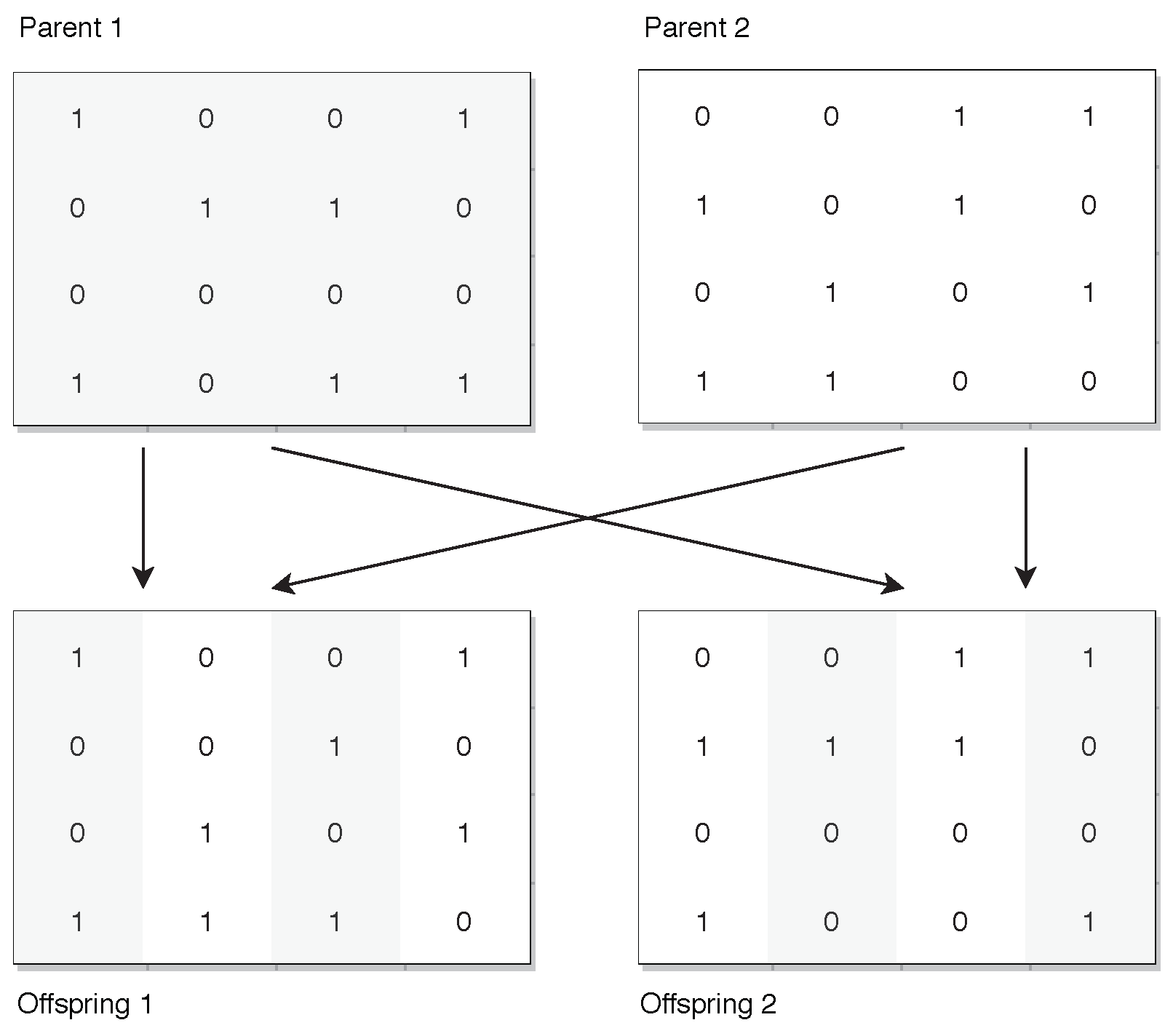
First, we introduce the proposed evolutionary operators of crossover and mutation and the unfeasible solution repair method for the ISHOP-U.

5.1.1. Crossover

The purpose of the crossover operator is to exploit the search space regions near promissory solutions. Our proposed crossover operator is similar to the principle of uniform recombination. For each j column, the crossover algorithm selects one parent randomly out of two possible parents. The selected parent copies its j column in the first offspring, and the non-selected parent copies its jth column to the second offspring. The crossover is graphically shown below (Figure 1).
The main advantage of the above crossover operator is that the offspring solutions are always feasible because the required item units for the jth product are preserved as in their original parents. Another advantage is that both parent solutions contribute similarly to the offspring genes, speeding up the gene stability in the population (exploitation).
The complexity of the crossover operator is linear and is equal to visiting every position of the matrix candidate solution O ( n m ) .

5.1.2. Mutation

The mutation operator is used to diversify the search, exploring new search space regions. The proposed mutation operator uses a mutation probability p m of changing the jth product demand in the ith store. The procedure is shown in Algorithm 3. The loops in Lines 1 and 2 control the indices j and i for the columns and rows in S, respectively. At every position s i , j , a random number r a n d U [ 0 , 1 ] is generated; if r a n d p m , then the value of s i , j is perturbed. The perturbation method changes the value of s i , j for a random value between zero and the minimum, between the required units for the product and their original value.
Algorithm 3 Proposed mutation operator for the ISHOP with item units.
1:
for j = 1 to n do
2:
      for  i = 1 to m do
3:
            if  r a n d p m  then
4:
              a Number of units required for the product j
5:
              b a i , j
6:
             if  a < b  then
7:
                a b a
8:
             else
9:
                a b b
10:
             end if
11:
              s i , j random integer [ 0 , a b ]
12:
            end if
13:
      end for
14:
end for
The proposed mutation process avoids the effect of adding unnecessary units of products by selecting an upper bound for s i , j , the minimum between the available units a i , j in the store i and the total required units l j of j product. Once the mutation finishes, the solutions are commonly unfeasible. Therefore, we repair the solutions in a separate algorithm, adding more diversity to the process.
The complexity of the mutation operator is linear and is equal to visiting every position of the matrix candidate solution O ( n m ) .

5.1.3. Solution Repair

Our proposed Algorithm 4 repairs unfeasible solutions, producing feasible and more diverse solutions. After the perturbation process in Algorithm 3, the candidate solution could be unfeasible. The core idea behind Algorithm 4 is that the sum of the elements in the jth column has to equal the total number of units required l j for the jth product. Consequently, the main loop in Algorithm 4 controls the j index for the products/columns and a second inner loop controls the i index for the stores/rows.
Algorithm 4 Proposed solution repair for the ISHOP with item units.
1:
for j = 1 to n do
2:
      s u m 0
3:
     for  i = 1 to m do
4:
        if  s i , j > a i , j  then
5:
            s i , j a i , j
6:
        end if
7:
         s u m s u m + s i , j
8:
     end for
9:
     while  s u m < l j  do
10:
        Select a random store i with available units
11:
         s i , j s i , j + 1
12:
         s u m s u m + 1
13:
     end while
14:
     while  s u m > l j  do
15:
        Select a random store i where s i , j > 0
16:
         s i , j s i , j 1
17:
         s u m s u m 1
18:
     end while
19:
end for
At every j column, the sum of the selected units to buy from the stores should equal the total required units l j (Line 9). If the sum is lower than the required units, the repair procedure selects random stores to buy units from which still have available units. In case the sum is greater than the total required units l j (Line 14), the repair procedure will randomly remove individual units of the j column from an i store, where the number of required units is higher than zero ( s i , j > 0 ).

5.2. Genetic Algorithm

Genetic Algorithms (GAs) are a popular optimization technique for combinatorial and continuous problems [14]. GAs evolve a population of initial random candidate solutions, through sexual reproduction and mutations, as in Darwinian evolution. Figure 2 shows the generic framework of GAs.
The first step in a GA is to select individuals for reproduction from the population, also known as parent selection, and the second step is to use the recombination operator of crossover (Section 5.1.1) and mutation (Section 5.1.2) to produce new individuals. Finally, a process called environmental selection removes the individuals with the worst fitness, leaving only the ones with the best objective values; in our case, the ones with the lowest final purchase price. Each iteration of the main loop is called a generation and usually produces an equal number of new individuals as in the initial population. Environmental selection is responsible for keeping the population size constant and selecting the best-fitted individuals. Our proposed GA follows the abovementioned principles using our proposed crossover, mutation, and repair methods for the ISHOP-U.

5.3. Cellular Genetic Algorithm

Cellular Genetic Algorithms (CGAs) are a variant of the canonical GAs with a structured population. Canonical GAs use a panmictic population, where individuals can mate with any other in the population. On the contrary, CGAs restrict the possible mate partners based on a small proximity neighborhood. The CGAs neighborhoods overlap, providing exploration in the search space (diversification), while exploitation takes place inside each proximity neighborhood (intensification) [15,16]. The idea of using a non-panmictic population is to have a higher genetic differentiation, avoiding stagnation in the search. Figure 3 shows the most used neighborhoods in CGAs with the population structured as a grid.
Analogously, CGA follows the core evolutionary operations of a canonical GA (selection, crossover, mutation). Figure 4 shows the pseudocode of the CGA, where the difference lies in managing a structured population. A common approach is to replace the solutions of the current grid population with their corresponding ones in the offspring grid population if these outperform them. At every generation, the positions in the grid (see Figure 3) are visited in sequential order from the first individual to the last one ( P o p S i z e ). Then, the algorithm selects individuals for recombining exclusively from their current neighborhood. After the crossover procedure, a single solution is mutated, evaluated, and store in its equivalent grid position in an auxiliary offspring population. Unlike GAs that use an environmental selection over the current and offspring populations, The CGA’s replacement method is similar to the one used in Differential Evolution [17].

6. Experimental Setup

This section describes the studied set of instances (Section 6.1), the tuning of the proposed evolutionary algorithms (Section 6.2), the algorithms for comparison (Section 6.5), and the statistical validations of the experiment (Section 6.6).

6.1. Proposed Synthetic Benchmark

To evaluate our proposed formulation, we generate a set of synthetic instances of different sizes for the ISHOP-U of three subsets with five instances: a small (10 products with 25 stores), a medium (25 products with 50 stores), and a large (50 products with 100 stores). The delivery prices vary within the range [0, 10], while the product prices oscillate in the range [5, 50] for all the instances. The prices follow a random uniform distribution. The benchmark of 15 synthetic instances can be download from [18]. The generation of a new instance starts by requesting the following:
  • The number of products and their required units;
  • The number of stores;
  • The maximum and minimum values for product costs;
  • The maximum and minimum for the delivery costs.
A store’s available units are random between 0 and the maximum required units. After this, each store has a random delivery cost and product price between their minimum and maximum value. Large instances consist of 2500 entries with 50 products in 100 stores, medium instances contain 625 entries with 25 products in 50 stores, and small instances have 125 entries with 10 products in 25 stores. All instances have a cost per product between 5 and 50 and a delivery cost between 0 and 10.

6.2. Evolutionary Algorithms Tuning

The parameter setting of the proposed algorithms was configured through exhaustive experimentation. We evaluate different combinations of recombination p r = { 1.0 , 0.9 , 0.8 , 0.7 , 0.6 } and mutation p m = { 0.05 , 0.10 , 0.15 , 0.20 , 0.25 } probabilities. The above produces a total of 25 possible configurations in the studied EAs. After evaluating the 25 configurations in both algorithms (GA and CGA), we conclude that the same best configuration is p r = 1.0 , p m = 0.05 . The population size of the algorithms is fixed to 100, a commonly used setting in the EAs literature. As a stop condition, we set a maximum of 25,000 objective function evaluations, equivalent to 250 generations in EAs with a population size of 100. The parameter settings are summarized in Table 5.

6.3. Sensitivity Analysis

To analyze the parameter sensitivity behavior of the proposed EAs, we perform a parameter analysis using as a reference the best parameter setting ( p r = 1.0 , p m = 0.05 ). We graphically analyze the median fitness evolution (on 100 independent runs) for all configurations. First, we analyze the crossover rate sensitivity, using parameters p r = { 1.0 , 0.9 , 0.8 , 0.7 , 0.6 } in Figure 5 for the GA. Here, we can see that the GA’s sensitivity to the crossover rate is low. For the instances Small 1 and Small 2 , all configurations converge, and for the instances Large 1 and Large 2 , the final performances differ. Clearly, the best crossover rate for the GA is p r = 1.0 in Figure 5.
The GA is very sensitive to the mutation rate. We graphically show the fitness evolution for the mutation rates p m = { 0.05 , 0.10 , 0.15 , 0.20 , 0.25 } in Figure 6. The graphical analysis shows that the lower the mutation rate, the faster the algorithm convergence to the best final performance. This behavior is directly related to the aggressive mutation mechanism described in Section 5.1.2. After applying a mutation, there is a huge possibility that the solution would be unfeasible. The solution would thus need to be repaired, diversifying it more. Therefore, the higher the mutation rate, the higher the elitist genetic information lost. Based on the results in Section 7 we recommend elitism to solve the ISHOP-U.
Figure 7 concentrates the graphical results for crossover and mutation rates sensitivity analysis for CGA. The results for CGA are consistent with the results found for GA. The best crossover rate is p r = 1.0 , and the best mutation rate is p m = 0.05 . Although both algorithms’ convergence speeds and final performances are different, their sensitivity behavior to the parameters is comparable. All the crossover rates in the CGA equally converge for the instances Small 1 and Small 2 . While for Large 1 and Large 5 , the convergence speed and final performance differ. The CGA is also very sensitive to the mutation rates; the lower the mutation rate, the best the convergence speed and final performance.

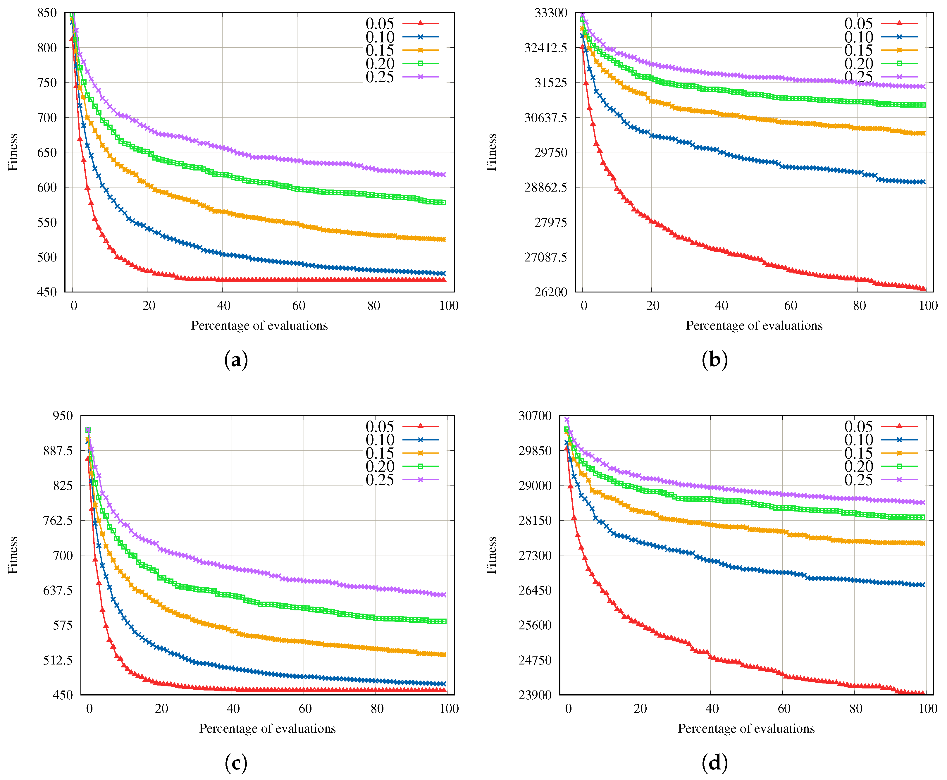
6.4. Convergence Analysis

In this section, we analyze the convergence of the two proposed EAs. We select four representative instances of the synthetic benchmark to carry on our analysis (Small 1 , Small 2 , Large 1 , Large 5 ), the ones with the lowest and highest IQR results in the primary experimentation. We plot the fitness evolution during the search of the GA and CGA in Figure 8, sampling every 250 objective function evaluations (100 points) in the graphs. Figure 8 shows that both algorithms converge at almost the same values for Small 1 and Small 2 instances; the instances have a search space of size 25 10 (10 products in 25 stores), sufficient for a satisfactory convergence on the 25,000 function evaluations in both EAs. However, to achieve convergence in Large 1 and Large 5 , which have a search space 100 50 (50 products in 100 stores), 25,000 evaluations are not enough. The GA achieves the best result on Large 1 and Large 2 .
With these results, we can conclude that the difference in the final achieved quality between the GA and CGA increases with the size of the search space. The bigger the search space, the more significant the difference in their final performances.

6.5. Algorithms for Comparison

In order to validate the competitive performance of the two proposed EAs, we reproduce the best representative algorithm from the ISHOP-U in the state-of-the-art: the Water Cycle Algorithm proposed by Sadollah et al. [9]. We use as a base for the ISHOP-U problem implementation the original Ali Sadollah (2022) Water Cycle Algorithm (WCA), Unconstrained Discrete Version 2, available at https://www.mathworks.com/matlabcentral/fileexchange/58011-water-cycle-algorithm-wca-unconstrained-discrete-version-2 (accessed on 10 June 2022). The WCA parameter settings are tuned as recommended by the author.

6.6. Statistical Validations

Due to the stochastic nature of the algorithms, we perform 100 independent executions on every instance from the proposed synthetic benchmark in Section 6.1.
Recently, the research community has presented concerns and criticism about the Null Hypothesis Statistical Tests (NHST), as stated in [19]. Among the main criticisms, we find two: (i) the NHST gives no direct information about the superiority of an algorithm over another one, only looking for a significative difference, and (ii) the ability to reject the null hypothesis with many experimental observations even with a tiny difference, also known as effect size. Therefore, to avoid the drawbacks of using NHST, we perform Bayesian statistical tests [20]. The Bayesian paradigm computes a distribution of the parameter of interest (performance) for making statements about the difference in the distributions of the comparison algorithms. To assess statistical significance, in a pairwise comparison between the algorithms, we performed the Bayesian Wilcoxon signed-rank test [21], which is an extension of the classical non-parametric Wilcoxon signed-rank test [22], evaluating for a significance level of α = 0.95 . Comparing two algorithms using the Bayesian Wilcoxon signed-rank test produces three probabilities as output: l e f t , r o p e , and r i g h t , where l e f t is the probability that differences lie in [ , r ] , r o p e in [ r , r ] , and right in [ r , ] , representing negative, equivalent, and positive differences, respectively, with regard to the rope value r. Given two optimization algorithms for minimization A and B, the first column being the data of A and the data of B the second column for the Bayesian test, we have four possible outcomes:
  • l e f t 0.95 : in this case, algorithm A outperforms B because their differences have a significant probability of being negative.
  • r i g h t 0.95 : in this case, algorithm B outperforms A because their differences have a significant probability of being positive.
  • r o p e 0.95 : in this case, algorithm A and B are equivalent.
  • When none of the above cases are true, the test does not have enough information, making an undecided statement.
We added to the results in Table 6 the statistical information between every algorithm (column A) and the WCA (column B) using the symbols §, †, ≈, and ? when the WCA is statistically outperformed, when the WCA statistically outperforms, when the algorithms are statistical equivalent, and for undecided cases, respectively. In addition, we compute the median values and their Interquartile Ranges (IQR) obtained by the GA, CGA, and WCA as central tendency and dispersion measures, respectively.
To analyze the performance of the algorithms in a multicomparison, we perform the Bayesian Friedman test [23], which is an extension of the Friedman non-parametric test [22,24]. Finally, to compare the global performance of the studied algorithms, we present the mean ranks produced by the Bayesian Friedman test.

7. Results and Discussion

The experimental results from Table 6 show the median ( x ˜ ) and IQR values for the main experiment. The best results are highlighted in dark gray, while the second-best are in light gray. From Table 6, it is clear that the GA outperforms the CGA in almost every instance from the synthetic benchmark. The underlying reason for these results could be the difference between the GA environmental selection and the CGA replacement policy. Canonical GAs tend to be more elitist, joining the current population with the offspring, thus removing the worst-fitted individuals. While CGAs depends on the replacement policy, in our case, the offspring can only replace an individual of the same position in the grid (if better fitted). Regarding the performance of the proposed EAs against the WCA, we see a clear tendency of the WCA to achieve best-median values when the instance size is considerably big (at least 50 products and 100 stores). In other words, EAs tend to be more diverse than WCA, but that extreme diversity plays against their performance on ISHOP-U large instances. We could confirm that less diversity is favorable because CGA is more diverse than canonical EAs and performs the worst. However, the Bayesian test shows indecision in the large instance set, and it is impossible to state that WCA outperforms the GA and CGA in the large instance set for a significant level of 95%. Furthermore, we compute the Bayesian Friedman test, confirming a 95% of statistical significance and computing the mean rankings as follows: in first place is the GA with 1.36, in second place is the CGA with 2.08, and in third place is the WCA with 2.56. The computed Friedman mean ranks are consistent with the number of times the GA and the CGA outperform the WCA with statistical significance (symbol §) in Table 6.

8. Conclusions

This work investigates the Internet Shopping Optimization Problem with item Units (ISHOP-U). We prove the ISHOP-U decision version is NP-complete, even in the simple case of one unit per product. Therefore, the optimization version of ISHOP-U is NP-hard. We propose two new evolutionary operators for the ISHOP-U, one for recombination and the other for mutation. Additionally, we propose one repair method for unfeasible solutions. We evaluated the proposed operators on two Evolutionary Algorithms, the GA and the CGA. The assessment of the implementations of both algorithms is compared against the results of a Water Cycle Algorithm, and both algorithms outperform it with statistical significance. Finally, based on the obtained results, we recommend more elitist and fewer diversity algorithms to solve the ISHOP-U.

Author Contributions

Conceptualization, A.S. and J.D.T.-V.; methodology, F.B. and J.L.-M.; software, F.O., A.S. and A.H.G.; validation, A.S., J.D.T.-V. and A.H.G.; formal analysis, A.S., F.B. and J.A.C.R.; investigation, J.L.-M. and M.G.T.-B.; resources, S.I.M. and J.A.C.R.; data curation, F.O., M.P.P.-F. and A.S.; writing—original draft preparation, S.I.M., M.P.P.-F., J.A.C.R. and J.L.-M.; writing—review and editing, A.H.G. and M.G.T.-B.; visualization, A.S. and M.P.P.-F.; supervision, A.S.; project administration, S.I.M.; funding acquisition, J.A.C.R. All authors have read and agreed to the published version of the manuscript.

Funding

A. Santiago would like to acknowledge the Mexican Council of Science and Technology (CONACyT Mexico) for the SNI salary award under the record 83525. The APC was funded by the Universidad Autónoma de Tamaulipas.

Institutional Review Board Statement

Not applicable.

Informed Consent Statement

Not applicable.

Data Availability Statement

The benchmark instances for this study are available at https://github.com/AASantiago/SchedulingInstances, accessed on 10 June 2022.

Conflicts of Interest

The authors declare no conflict of interest. The funders had no role in the design of the study; in the collection, analyses, or interpretation of data; in the writing of the manuscript, or in the decision to publish the results.

Abbreviations

The following abbreviations are used in this manuscript:
CGACellular Genetic Algorithm
EAEvolutionary Algorithm
GAGenetic Algorithm
ISHOPInternet Shopping Optimization Problem
ISHOP-UInternet Shopping Optimization Problem with item Units
WCAWater Cycle Algorithm
§ Statistically superior to WCA
?Statistical indecision to WCA
p Polynomial transformation

References

  1. Dailey, N. 2022 is Expected to be the First Trillion-Dollar Year for Online Sales, Largely Thanks to the COVID-19 Pandemic. 2021. Available online: https://www.businessinsider.com/ecommerce-sales-first-trillion-dollar-year-2022-covid-pandemic-adobe-2021-3?r=US&IR=T (accessed on 5 April 2021).
  2. Błazewicz, J.; Kovalyov, M.; Musiał, J.; Urbański, A.; Wojciechowski, A. Internet shopping optimization problem. Int. J. Appl. Math. Comput. Sci. 2010, 20, 385–390. [Google Scholar] [CrossRef] [Green Version]
  3. Garey, M.; Johnson, D. Computers and Intractability: A Guide to the Theory of NP-Completeness; Freeman, W.H., Ed.; W. H. Freeman and Company: New York, NY, USA, 1979. [Google Scholar]
  4. Blazewicz, J.; Bouvry, P.; Kovalyov, M.Y.; Musial, J. Internet shopping with price sensitive discounts. 4OR 2014, 12, 35–48, Erratum in 4OR 2014, 12, 403–406. [Google Scholar] [CrossRef] [Green Version]
  5. Marszalkowski, J. Budgeted Internet Shopping Optimization Problem. In Proceedings of the 7th Multidisciplinary International Conference on Scheduling: Theory and Applications (MISTA 2015), Prague, Czech Republic, 25–28 August 2015; pp. 885–887. [Google Scholar]
  6. Chung, J.B. Internet shopping optimization problem with delivery constraints. J. Distrib. Sci. 2017, 15, 15–20. [Google Scholar] [CrossRef]
  7. Musial, J.; Lopez-Loces, M.C. Trustworthy Online Shopping with Price Impact. Found. Comput. Decis. Sci. 2017, 42, 121–136. [Google Scholar] [CrossRef] [Green Version]
  8. Huacuja, H.J.F.; Morales, M.Á.G.; Locés, M.C.L.; Santillán, C.G.G.; Reyes, L.C.; Rodríguez, M.L.M. Optimization of the Internet Shopping Problem with Shipping Costs. In Fuzzy Logic Hybrid Extensions of Neural and Optimization Algorithms: Theory and Applications; Castillo, O., Melin, P., Eds.; Springer International Publishing: Cham, Swizerland, 2021; pp. 249–255. [Google Scholar] [CrossRef]
  9. Sayyaadi, H.; Sadollah, A.; Yadav, A.; Yadav, N. Stability and iterative convergence of water cycle algorithm for computationally expensive and combinatorial Internet shopping optimisation problems. J. Exp. Theor. Artif. Intell. 2019, 31, 701–721. [Google Scholar] [CrossRef]
  10. Józefczyk, J.; Ławrynowicz, M. Heuristic algorithms for the Internet shopping optimization problem with price sensitivity discounts. Kybernetes 2018, 47, 831–852. [Google Scholar] [CrossRef]
  11. Blazewicz, J.; Cheriere, N.; Dutot, P.F.; Musial, J.; Trystram, D. Novel dual discounting functions for the Internet shopping optimization problem: New algorithms. J. Sched. 2016, 19, 245–255. [Google Scholar] [CrossRef] [Green Version]
  12. Sadollah, A.; Gao, K.; Barzegar, A.; Su, R. Improved model of combinatorial Internet shopping optimization problem using evolutionary algorithms. In Proceedings of the 2016 14th International Conference on Control, Automation, Robotics and Vision (ICARCV), Phuket, Thailand, 13–15 November 2016; pp. 1–5. [Google Scholar] [CrossRef]
  13. Sipser, M. Introduction to the Theory of Computation, 3rd ed.; Course Technology: Boston, MA, USA, 2013. [Google Scholar]
  14. Reeves, C.R. Genetic Algorithms. In Handbook of Metaheuristics; Gendreau, M., Potvin, J.Y., Eds.; Springer: Boston, MA, USA, 2010; pp. 109–139. [Google Scholar] [CrossRef]
  15. Alba, E.; Dorronsoro, B. Cellular Genetic Algorithms; Springer Science & Business Media: Berlin/Heidelberg, Germany, 2009; Volume 42. [Google Scholar]
  16. Alba, E.; Dorronsoro, B. The exploration/exploitation tradeoff in dynamic cellular genetic algorithms. IEEE Trans. Evol. Comput. 2005, 9, 126–142. [Google Scholar] [CrossRef] [Green Version]
  17. Kenneth Price, R.M.S.; Lampinen, J.A. The Differential Evolution Algorithm. In Differential Evolution: A Practical Approach to Global Optimization; Springer: Berlin/Heidelberg, Germany, 2005; pp. 37–134. [Google Scholar] [CrossRef]
  18. Santiago, A.; Terán-Villanueva, J.D.; Martínez, S.I.; Ornelas, F.; Ponce-Flores, M. Benchmark Instances for: The Internet Shopping Optimization Problem with Item Units (ISHOP-U): Formulation, Instances, NP-Completeness, and Evolutionary Algorithms. 2021. Available online: https://github.com/AASantiago/ISHOP-U-Instances (accessed on 5 April 2021).
  19. Carrasco, J.; García, S.; Rueda, M.; Das, S.; Herrera, F. Recent trends in the use of statistical tests for comparing swarm and evolutionary computing algorithms: Practical guidelines and a critical review. Swarm Evol. Comput. 2020, 54, 100665. [Google Scholar] [CrossRef] [Green Version]
  20. Benavoli, A.; Corani, G.; Demšar, J.; Zaffalon, M. Time for a Change: A Tutorial for Comparing Multiple Classifiers through Bayesian Analysis. J. Mach. Learn. Res. 2017, 18, 1–36. [Google Scholar]
  21. Benavoli, A.; Corani, G.; Mangili, F.; Zaffalon, M.; Ruggeri, F. A Bayesian Wilcoxon signed-rank test based on the Dirichlet process. In Proceedings of the International Conference on Machine Learning, PMLR, Bejing, China, 22–24 June 2014; pp. 1026–1034. [Google Scholar]
  22. Corder, G.W.; Foreman, D.I. Nonparametric Statistics for Non-Statisticians; John Wiley & Sons, Inc.: Hoboken, NJ, USA, 2011. [Google Scholar]
  23. Benavoli, A.; Corani, G.; Mangili, F.; Zaffalon, M. A Bayesian Nonparametric Procedure for Comparing Algorithms. In Proceedings of the International Conference on Machine Learning, PMLR, Lille, France, 7–9 July 2015; pp. 1264–1272. [Google Scholar]
  24. Santiago, A.; Ponce-Flores, M.; Terán-Villanueva, J.D.; Balderas, F.; Martínez, S.I.; Rocha, J.A.C.; Menchaca, J.L.; Berrones, M.G.T. Energy Idle Aware Stochastic Lexicographic Local Searches for Precedence-Constraint Task List Scheduling on Heterogeneous Systems. Energies 2021, 14, 3473. [Google Scholar] [CrossRef]
Figure 1. Graphical representation of the proposed crossover for the ISHOP with item units.
Mathematics 10 02513 g001
Figure 2. Genetic Algorithm (GA) framework.
Mathematics 10 02513 g002
Figure 3. Common neighborhoods in Cellular Genetic Algorithms, a black square represent the current solution, black circles their neighbor solutions.
Mathematics 10 02513 g003
Figure 4. Cellular Genetic Algorithm (CGA) framework.
Mathematics 10 02513 g004
Figure 5. Crossover rate sensitivity for the GA. (a) Instance 1 from the small set (Small 1 ). (b) Instance 1 from the large set Large 1 . (c) Instance 2 from the small set (Small 2 ). (d) Instance 5 from the large set (Large 5 ).
Mathematics 10 02513 g005
Figure 6. Mutation rate sensitivity GA. (a) Instance 1 from the small set (Small 1 ). (b) Instance 1 from the large set (Large 1 ). (c) Instance 2 from the small set (Small 2 ). (d) Instance 5 from the large set (Large 5 ).
Mathematics 10 02513 g006
Figure 7. Crossover and mutation rates fitness evolution for the CGA. (a) Instance Small 1 crossover rates. (b) Instance Large 1 crossover rates. (c) Instance Small 2 crossover rates. (d) Instance Large 5 crossover rates. (e) Instance Small 1 mutation rates. (f) Instance Large 1 mutation rates. (g) Instance Small 2 mutation rates. (h) Instance Large 5 mutation rates.
Mathematics 10 02513 g007
Figure 8. Comparison of the fitness evolution of the GA and CGA for some representative instances. (a) Instance 1 from the small set (Small 1 ). (b) Instance 5 from the large set (Large 5 ). (c) Instance 2 from the small set (Small 2 ). (d) Instance 1 from the large set (Large 1 ).
Mathematics 10 02513 g008
Table 1. Book prices and delivery costs offered by six Internet stores.
ABCDEDelivery
Store 1183929485910
Store 2244523544415
Store 3224523535315
Store 4284017574610
Store 5244224475910
Store 6274820555315
Table 2. Available book units offered in the six Internet stores.
ABCDE
Store 133258
Store 246874
Store 324547
Store 487862
Store 562383
Store 678932
Table 3. Units required of books (A–E) by the customer.
ABCDE
Units46872
Table 4. Feasible candidate solution.
ABCDE
Store 133000
Store 200802
Store 300000
Store 403000
Store 510070
Store 600000
Table 5. Parameter setting for GA and CGA algorithms.
GACGA
Population size:100100
MaxEvaluations:25,00025,000
Selection:Binary TournamentBinary Tournament
Neighborhood:L5
Recombination: p r = 1.0 , See Section 5.1.1 p r = 1.0 , See Section 5.1.1
Mutation: p m = 0.05 , See Algorithm 3 p m = 0.05 , See Algorithm 3
Table 6. Median and IQR of the GA, CGA, and RS over 100 independent runs. Dark and light gray emphasize the best and second-best results, respectively.
GACGAWCA
Instance x ˜ IQR x ˜ IQR x ˜ IQR
Small 1 467.04  § 0.0467.04  § 0.0580.1747.03
Small 2 457.64  § 0.41458.05  § 0.69552.141.57
Small 3 585.75  § 0.0587.85  § 2.84726.4152.11
Small 4 479.69  § 1.47483.07  § 4.43576.0141.8
Small 5 520.69  § 0.97522.88  § 3.35605.3535.26
Medium 1 3505.7  § 128.353709.77  § 133.444107.11244.68
Medium 2 4728.01  § 140.844943.86  § 134.125383.6307.62
Medium 3 5234.51  § 169.265486.86  § 166.025866.06349.54
Medium 4 4861.51  § 149.795111.59  § 152.315497.51278.68
Medium 5 5646.67  § 182.275934.77  § 168.396333.05336.3
Large 1 26,415.55  ? 522.6226,886.7  ? 521.8425,711.61042.82
Large 2 22,002.78  ? 469.422,462.82  ? 494.0121,675.881047.13
Large 3 21,983.9  ? 523.4222,487.28  ? 457.8921,869.36731.65
Large 4 24,172.27  ? 479.0924,620.75  ? 542.3624,202.27875.79
Large 5 24,039.28  ? 536.1524,543.6  ? 475.823,875.341000.51
§—Statistically superior to WCA; ? —Statistical indecision to WCA.
Publisher’s Note: MDPI stays neutral with regard to jurisdictional claims in published maps and institutional affiliations.

