Article

Multisensor Fusion Estimation for Systems with Uncertain Measurements, Based on Reduced Dimension Hypercomplex Techniques

by
Rosa M. Fernández-Alcalá
*,
José D. Jiménez-López
,
Jesús Navarro-Moreno
and
Juan C. Ruiz-Molina
Department of Statistics and Operations Research, University of Jaén, Paraje Las Lagunillas, 23071 Jaén, Spain
*
Author to whom correspondence should be addressed.
Mathematics 2022, 10(14), 2495; https://doi.org/10.3390/math10142495
Submission received: 8 June 2022 / Revised: 5 July 2022 / Accepted: 15 July 2022 / Published: 18 July 2022

Abstract

:
The prediction and smoothing fusion problems in multisensor systems with mixed uncertainties and correlated noises are addressed in the tessarine domain, under T k -properness conditions. Bernoulli distributed random tessarine processes are introduced to describe one-step randomly delayed and missing measurements. Centralized and distributed fusion methods are applied in a T k -proper setting, k = 1 , 2 , which considerably reduce the dimension of the processes involved. As a consequence, efficient centralized and distributed fusion prediction and smoothing algorithms are devised with a lower computational cost than that derived from a real formalism. The performance of these algorithms is analyzed by using numerical simulations where different uncertainty situations are considered: updated/delayed and missing measurements.

1. Introduction

Multisensor systems and data fusion techniques are receiving increasing research and practical attention due to their ability to provide more robust estimation procedures than those that use a single sensor, as well as their broad applications in fields such as robotics, image processing, autonomous navigation, and smart homes, among others [1,2,3,4,5]. In estimation problems from noisy sensor measurements, the best known and most widely applied procedure is the Kalman filter and its different extensions, which are based on a state–space system (see, for example, [5,6,7,8]).
Of great interest are those systems that incorporate the effect of possible uncertainties into the measurements caused by physical failures in the sensors and measurement noises as well as failures in data transmission, all of which result in random delayed and missing measurements.
These uncertainties can be modeled by using stochastic parameters, being widely spread to consider Bernoulli distributed random processes. In these uncertainty scenarios, an extensive literature exists on the design of efficient recursive estimation algorithms (see, e g., [9,10,11,12,13,14,15], and references therein).
Depending on how raw data from different sensors are processed, two fundamental multisensor information fusion approaches are used: centralized and distributed fusion methods. In the centralized fusion structure, data coming from multiple sources are directly sent to a single fusion center, where the optimal estimator can be obtained, whereas in the distributed fusion strategy, these data are independently transmitted to individual nodes where local estimators are computed and sent in a second layer to the fusion center, producing robust and reliable estimators with a lower computational cost. These two approaches have been extensively studied in the real field, and both centralized and distributed fusion estimation algorithms have been designed under different initial hypotheses. Specifically, when the signal to be estimated is modeled by a state–space model with uncertain measurements, filtering, prediction, and smoothing algorithms have been proposed in [9,10,11] from a centralized fusion perspective and in [13,14,15] by applying distributed fusion techniques.
Alternatively, the multisensor fusion estimation problem has also been analyzed by using 4D hypercomplex algebras [16,17,18,19,20,21,22,23]. These algebras appear to be a natural extension of complex algebras comprising a real part and three imaginary parts, which gives rise to ideal structures for describing phenomena in the real physical world. Moreover, the use of these algebras in different practical problems has revealed their supremacy over their treatment in the real space [24,25,26,27]. In this field, quaternions have been the most common 4D hypercomplex algebra in signal processing, since they have the desirable property of being a normed division algebra. Unlike quaternions, tessarines constitute a commutative algebra which facilitates the extension of the main results obtained in the real and complex fields to the four-dimensional case, and the use of tessarines as a signal processing tool has been gaining popularity in the last few years [22,23,28].
In general, the most suitable processing for these signals is the widely linear processing (WL) based on four-dimensional augmented vectors given by the signal itself and its three principal conjugations. Nevertheless, some properness properties related to the vanishing of the complementary functions make it possible to determine the type of processing to be used, which is based on reduced-dimensional processes that lead to computational savings without losing accuracy. This computational cost reduction cannot be achieved from a real formalism [24,29,30,31].
In the tessarine domain, two types of properness have recently been introduced, namely T 1 and T 2 -properness [24,32], and they have been satisfactorily applied in multisensor fusion estimation problems with uncertainties in the measurements [22,23]. In [22], T k -proper, k = 1 , 2 , centralized fusion algorithms of reduced dimension are proposed for the computation of the optimal (in the least-squares sense) filter, predictor, and fixed-point smoother of the state in systems with random one-step delays and correlated noises. In [23], a more general problem with random sensor delays and missing measurements is analyzed. Under T k -properness conditions, k = 1 , 2 , the authors have devised computationally efficient centralized and distributed fusion filtering algorithms by considering the LS distributed weighted fusion criterion. However, the prediction and smoothing problems remain to be solved.
Therefore, our aim in this paper is to address the prediction and smoothing problems under T k -properness conditions, k = 1 , 2 , from both centralized and distributed approaches. As in [23], the state to be estimated is assumed to be observed through a state–space model with correlated noises, where measurements may be updated, one-step delayed, or contain only noise according to Bernoulli tessarine random variables. In this setting, both centralized and distributed fusion prediction and smoothing algorithms are provided. The advantage of these algorithms is that they have a lower computational load than their counterparts derived from a real processing. The behavior of these algorithms is numerically analyzed for different uncertainty scenarios by means of simulation examples, in which the prediction and smoothing results are also compared with the filter.
With this purpose, the remainder of the paper is structured as follows: Section 2 presents the basic concepts and properties regarding the signal processing in the tessarine field. In Section 3, the multisensor fusion estimation problem for systems with random one-step sensor delays and missing measurements is formulated in the tessarine domain, by considering a T k -proper scenario, k = 1 , 2 . Section 4 and Section 5 provide, respectively, the T k -proper distributed and centralized fusion estimation algorithms for the computation of the corresponding prediction and smoothing estimators, as well as their mean square errors. Specifically, in Section 4, the least squares (LS) local estimators are first determined, and in a second layer, a weighted linear combination of these local estimators, in LS sense, is used to generate the distributed fusion estimators.
Afterwards, Section 6 includes numerical simulations to illustrate the performance of the proposed algorithms in different settings: both T 1 -proper and T 2 -proper scenarios, different uncertainty situations (one-step delay, missing measurements, and mixed uncertainties), centralized and distributed fusion methods, and different prediction and smoothing problems. Finally, the main conclusions of the paper are drawn in Section 7. For the sake of readability, all the proofs have been moved to Appendix A, Appendix B, Appendix C and Appendix D.
Notation: The notation used throughout this paper is fairly standard. The superscripts “*”, “ T ”, and “ H ” denote the tessarine conjugate, transpose, and Hermitian transpose. Boldface uppercase letters refer to matrices, boldface lowercase letters refer to column vectors, and lightface lowercase letters are used for scalar quantities. In particular, 0 n × m represents the n × m zero matrix, I n is the identity matrix of dimension n, and 1 n (respectively, 0 n ) is the column vector of dimension n whose elements are all 1 (respectively, 0). Moreover, Z , R and T represent the set of integer, real, and tessarine numbers, respectively. Then, A R n × m (respectively, A T n × m ) indicates that A is a real (respectively, tessarine) n × m matrix, and a R n (respectively, a T n ) means that a is a n-dimensional real (respectively, tessarine) vector. Additionally, E [ · ] and Cov ( · ) are the expectation and covariance operators, respectively; diag ( · ) is a diagonal (or block diagonal) matrix with entries (block entries) on the main diagonal. Finally, “∘” and “⊗” symbolize the Hadamard and Kronecker products, respectively, and δ t s , is the Kronecker delta function.

2. Tessarine Processing

The tessarine domain is a commutative extension of the complex domain comprising a real part and three imaginary parts [28]. In this section, the main concepts and properties present in the tessarine domain are established.
Note that, unless otherwise stated, all the random variables are assumed to have zero-mean throughout this paper.
Definition 1.
A tessarine random signal vector x ( t ) T n can be defined as a stochastic process of the form [32]
x ( t ) = x r ( t ) + η x η ( t ) + η x η ( t ) + η x η ( t ) , t Z ,
with x ν ( t ) R n , for ν = r , η , η , η , real random signal vectors, and the triad { η , η , η } satisfying the following identities:
η η = η , η η = η , η η = η , η 2 = η 2 = 1 , η 2 = 1 .
Definition 2.
The pseudo-autocorrelation function of x ( t ) T n is defined as R x ( t , s ) = E [ x ( t ) x H ( s ) ] , t , s Z , and the pseudo-cross-correlation function of x ( t ) , y ( t ) T n as R x y ( t , s ) = E [ x ( t ) y H ( s ) ] , t , s Z .
Given a random signal x ( t ) T n , the real vector formed by its components is denoted by
x r ( t ) = x r T ( t ) , x η T ( t ) , x η T ( t ) , x η T ( t ) T , t Z .
Moreover, the conjugate of x ( t ) is defined as
x * ( t ) = x r ( t ) η x η ( t ) + η x η ( t ) η x η ( t ) ,
and the following auxiliary tessarines are introduced:
x η ( t ) = x r ( t ) + η x η ( t ) η x η ( t ) η x η ( t ) , x η ( t ) = x r ( t ) η x η ( t ) η x η ( t ) + η x η ( t ) .
For a complete description of the second-order statistics of x ( t ) , the augmented tessarine signal vector x ¯ ( t ) = [ x T ( t ) , x * T ( t ) , x η T ( t ) , x η T ( t ) ] T might be defined, which satisfies the following relationship with x r ( t ) :
x ¯ ( t ) = 2 T x r ( t ) ,
where T = 1 2 A I n , with
A = 1 η η η 1 η η η 1 η η η 1 η η η ,
and where T H T = I 4 n .
In this context, based on the vanishing of the different pseudo-correlation functions R x x ν ( t , s ) , ν = * , η , η ,29,32] introduced two interesting types of properness, named T 1 and T 2 -properness, which are included in the following definition.
Definition 3.
A random signal x ( t ) T n is T 1 -proper (respectively, T 2 -proper) if, and only if, R x x ν ( t , s ) , with ν = * , η , η (respectively, ν = η , η ), vanish t , s Z .
Analogously, two random signals x ( t ) T n 1 and y ( t ) T n 2 are cross T 1 -proper, (respectively, cross T 2 -proper) if, and only if, R x y ν ( t , s ) , with ν = * , η , η (respectively, ν = η , η ), vanish t , s Z .
Finally, x ( t ) and y ( t ) are jointly T 1 -proper (respectively, jointly T 2 -proper) if, and only if, they are T 1 -proper (respectively, T 2 -proper) and cross T 1 -proper (respectively, cross T 2 -proper).
Note that the T 1 and T 2 -properness properties have a direct impact on the signal processing approach. Thus, the optimal linear processing in the tessarine domain is the widely linear (WL) processing that entails operating on the augmented tessarine vector x ¯ ( t ) T 4 n . Nevertheless, under T k -properness conditions, k = 1 , 2 , the WL processing is reduced to a T k -proper linear processing, which implies a considerable reduction in the dimension of the processes involved. Particularly, T 1 -proper linear processing considers the tessarine random signal itself, x ( t ) T n , and T 2 -proper linear processing takes into account the 2 n -dimensional augmented vector given by the signal and its conjugate [29].
Definition 4.
Given two random tessarine signal vectors x ( t ) , y ( s ) T n , the productbetween them is defined as
x ( t ) y ( s ) = x r ( t ) y r ( s ) + η x η ( t ) y η ( s ) + η x η ( t ) y η ( s ) + η x η ( t ) y η ( s ) .
Property 1.
The augmented vector of x ( t ) y ( s ) is x ( t ) y ( s ) ¯ = D x ( t ) y ¯ ( s ) , where D x ( t ) = T diag ( x r ( t ) ) T H .

3. Problem Statement

Consider a networked system given by an n-dimensional tessarine state x ( t ) T n which is observed from R sensors, each of which provides measurements z ( i ) ( t ) T n , i = 1 , , R , perturbed by additive noises. Specifically, this system is assumed to be described by the following state–space model:
x ( t + 1 ) = F 1 ( t ) x ( t ) + F 2 ( t ) x * ( t ) + F 3 ( t ) x η ( t ) + F 4 ( t ) x η ( t ) + u ( t ) , t 0 , z ( i ) ( t ) = x ( t ) + v ( i ) ( t ) , t 1 , i = 1 , , R ,
where F j ( t ) T n × n , j = 1 , , 4 , are deterministic matrices, and u ( t ) , v ( i ) ( t ) T n are correlated tessarine white noises with pseudo-variances Q ( t ) and R ( i ) ( t ) , respectively, and E [ u ( t ) v ( i ) H ( s ) ] = S ( i ) ( t ) δ t , s . Moreover, v ( i ) ( t ) is independent of v ( j ) ( t ) , for any two sensors i j , and the initial state x ( 0 ) , with E [ x ( 0 ) x H ( 0 ) ] = P 0 , is independent of u ( t ) and v ( i ) ( t ) , for t 0 , i = 1 , , R .
Remark 1.
Unlike the state–space systems considered in the conventional linear processing, which only use the information supplied by the signal itself, the state equation in (1) captures the full second-order information available in the state transmission.
The measurements available from each sensor are assumed to be affected by random network-induced delay and missing measurements, according to the following model:
y ( i ) ( t ) = γ 1 ( i ) ( t ) z ( i ) ( t ) + γ 2 ( i ) ( t ) z ( i ) ( t 1 ) + ( 1 n γ 1 ( i ) ( t ) γ 2 ( i ) ( t ) ) v ( i ) ( t ) , t 2 , y ( i ) ( 1 ) = z ( i ) ( 1 ) .
For each sensor i = 1 , , R and, for j = 1 , 2 , γ j ( i ) ( t ) = [ γ j 1 ( i ) ( t ) , , γ j n ( i ) ( t ) ] T T n is a tessarine random vector whose elements γ j m ( i ) ( t ) , for m = 1 , , n , are composed of independent Bernoulli random variables, γ j m , ν ( i ) ( t ) , with ν = r , η , η , η , with known probabilities p j m , ν ( i ) ( t ) , which indicate whether the corresponding component of the available measurement is updated ( γ 1 m , ν ( i ) ( t ) = 1 ), one-step delayed ( γ 2 m , ν ( i ) ( t ) = 1 ), or only contains noise ( γ 1 m , ν ( i ) ( t ) = γ 2 m , ν ( i ) ( t ) = 0 ).
The following hypotheses on the Bernoulli random variables are assumed:
  • For each i = 1 , , R , m = 1 , , n , ν = r , η , η , η , they must satisfy that γ 1 m , ν ( i ) ( t ) + γ 2 m , ν ( i ) ( t ) = 1 or γ 1 m , ν ( i ) ( t ) + γ 2 m , ν ( i ) ( t ) = 0 at every instant of time, i.e., if one of them takes the value 0, the other one is 1, or both are 0.
  • p 1 m , ν ( i ) ( t ) + p 2 m , ν ( i ) ( t ) 1 , for every i = 1 , , R , m = 1 , , n , ν = r , η , η , η .
  • For each sensor i = 1 , R , and j = 1 , 2 , γ j ( i ) ( t ) and γ j ( i ) ( s ) are independent for s t , and also γ j ( i ) ( t ) and γ j ( l ) ( t ) are independent for i l .
  • γ j ( i ) ( t ) is independent of x ( t ) , u ( t ) and v ( l ) ( t ) , for any i , l = 1 , , R .
In this setting, we consider the optimal (in the least-squares sense) linear estimation problem of the state x ( t ) on the basis of the measurements available from the R sensors: { y ( i ) ( 1 ) , , y ( i ) ( s ) } , i = 1 , , R .
To exploit the complete second-order statistical information available, the augmented statistics should be considered. With this purpose, the following WL model is defined from (1), (2), and Property 1:
x ¯ ( t + 1 ) = Φ ¯ ( t ) x ¯ ( t ) + u ¯ ( t ) , t 0 ,
z ¯ ( i ) ( t ) = x ¯ ( t ) + v ¯ ( i ) ( t ) , t 1 ,
y ¯ ( i ) ( t ) = D γ 1 ( i ) ( t ) z ¯ ( i ) ( t ) + D γ 2 ( i ) ( t ) z ¯ ( i ) ( t 1 ) + D 1 γ 1 ( i ) γ 2 ( i ) ( t ) v ¯ ( i ) ( t ) , t 2 ,
with y ¯ ( i ) ( 1 ) = z ¯ ( i ) ( 1 ) , and where
Φ ¯ ( t ) = F 1 ( t ) F 2 ( t ) F 3 ( t ) F 4 ( t ) F 2 * ( t ) F 1 * ( t ) F 4 * ( t ) F 3 * ( t ) F 3 η ( t ) F 4 η ( t ) F 1 η ( t ) F 2 η ( t ) F 4 η ( t ) F 3 η ( t ) F 2 η ( t ) F 1 η ( t ) .
Moreover, E u ¯ ( t ) u ¯ H ( t ) = Q ¯ ( t ) , E v ¯ ( i ) ( t ) v ¯ ( i ) H ( t ) = R ¯ ( i ) ( t ) , E u ¯ ( t ) v ¯ ( i ) H ( t ) = S ¯ ( i ) ( t ) , and E x ¯ ( 0 ) x ¯ H ( 0 ) = P ¯ 0 .
By considering that x ( t ) and y ( i ) ( t ) are jointly T k -proper, the available measurement Equation (5) can be rewritten in a reduced dimension form as follows:
y k ( i ) ( t ) = D k γ 1 ( i ) ( t ) z ¯ ( i ) ( t ) + D k γ 2 ( i ) ( t ) z ¯ ( i ) ( t 1 ) + D k 1 γ 1 ( i ) γ 2 ( i ) ( t ) v ¯ ( i ) ( t ) , t 2 ,
with y k ( i ) ( 1 ) = I k n , 0 k n × ( 4 k ) n z ¯ ( i ) ( 1 ) , and where
D k γ j ( i ) ( t ) = T k diag γ j ( i ) r ( t ) T H , i = 1 , , R , j = 1 , 2 , D k 1 γ 1 ( i ) γ 2 ( i ) ( t ) = T k diag 1 4 n γ 1 ( i ) r ( t ) γ 2 ( i ) r ( t ) T H , i = 1 , , R ,
with
T k = 1 2 B k I n ,
and
B k = 1 η η η , for k = 1 1 η η η 1 η η η , for k = 2 .
Moreover,
Π k γ j ( i ) ( t ) = E D k γ j ( i ) ( t ) = Π k j ( i ) ( t ) , 0 k n × ( 4 k ) n , i = 1 , , R , j = 1 , 2 , Π k 1 γ 1 ( i ) γ 2 ( i ) ( t ) = E D k 1 γ 1 ( i ) γ 2 ( i ) ( t ) = I k n Π k 1 ( i ) ( t ) Π k 2 ( i ) ( t ) , 0 k n × ( 4 k ) n , i = 1 , , R ,
where
Π 1 j ( i ) ( t ) = diag p j 1 , r ( i ) ( t ) , , p j n , r ( i ) ( t ) , i = 1 , , R , j = 1 , 2 , Π 2 j ( i ) ( t ) = 1 2 Π a j ( i ) ( t ) Π b j ( i ) ( t ) Π b j ( i ) ( t ) Π a j ( i ) ( t ) , i = 1 , , R , j = 1 , 2 ,
with
Π a j ( i ) ( t ) = diag p j 1 , r ( i ) ( t ) + p j 1 , η ( i ) ( t ) , , p j n , r ( i ) ( t ) + p j n , η ( i ) ( t ) , i = 1 , , R , j = 1 , 2 , Π b j ( i ) ( t ) = diag p j 1 , r ( i ) ( t ) p j 1 , η ( i ) ( t ) , , p j n , r ( i ) ( t ) p j n , η ( i ) ( t ) , i = 1 , , R , j = 1 , 2 .
Remark 2.
Note that the T k -properness means a reduction in the dimension of the available measurements by a half (if k = 2 ) or by a quarter (if k = 1 ).
Analagously, in a T 1 -proper setting, the processes x ¯ ( t ) , u ¯ ( t ) z ¯ ( i ) ( t ) , v ¯ ( i ) ( t ) and Φ ¯ ( t ) can be replaced by x 1 ( t ) x ( t ) , u 1 ( t ) u ( t ) , z 1 ( i ) ( t ) z ( i ) ( t ) , v 1 ( i ) ( t ) v ( i ) ( t ) , and Φ 1 ( t ) F 1 ( t ) ; and, in a T 2 -proper settings, they can be replaced by x 2 ( t ) x ( t ) , x H ( t ) T , u 2 ( t ) u ( t ) , u H ( t ) T , z 2 ( i ) ( t ) z ( i ) ( t ) , z ( i ) H ( t ) T , v 2 ( i ) ( t ) v ( i ) ( t ) , v ( i ) H ( t ) T and Φ 2 ( t ) = F 1 ( t ) F 2 ( t ) F 2 * ( t ) F 1 * ( t ) .
Furthermore, E u k ( t ) u k ( i ) H ( t ) = Q k ( i ) ( t ) , E v k ( t ) v k ( i ) H ( t ) = R k ( i ) ( t ) , E u k ( t ) v k ( i ) H ( t ) = S k ( i ) ( t ) , and E x k ( 0 ) x k H ( 0 ) = P 0 k .
This reduction in dimension results in computational savings in the estimation algorithms proposed, which cannot be attained from a real formalism.
In [23], conditions on the state–space model (3) which guarantee the T k -properness, for k = 1 , 2 , of the processes involved are provided.
Then, by considering T k -proper conditions, our aim is to obtain the LS linear estimator of the state x ( t ) from the set of measurements { y k ( i ) ( 1 ) , , y k ( i ) ( s ) } , i = 1 , , R . Recently, this problem has been solved for the case of t = s (filtering problem), providing both T k -proper centralized and distributed fusion filtering algorithms with similar performance to that obtained from a vectorial real approach but with a lower computational cost [23]. In this paper, this approach is extended to tackle the prediction (case t > s ) and smoothing (case t < s ) problems by using both centralized and distributed methods.

4. T k -Proper Distributed Fusion LS Linear Estimation

In this section, the distributed fusion LS linear estimation problem is addressed under T k -proper conditions.
The distributed fusion method consists of two steps: First, the measurements of each sensor are used to generate local LS linear estimators. Then, similar to the distributed fusion method used in [23], a fusion criterion based on weighted matrices in the LS sense is applied to generate the distributed fusion LS linear estimator as a linear combination of the local estimators. Next, these two steps are carried out.

4.1. Local T k -Proper LS Linear Estimation Algorithms

Consider the multisensor system given by (3), (4) and (6). The local T k -proper LS linear estimator of x ( t ) , denoted by x ^ ( i ) T k ( t | s ) is obtained by extracting the first n components of x ^ k ( i ) ( t | s ) , where x ^ k ( i ) ( t | s ) is given by the projection of x ¯ ( t ) onto the set of measurements { y k ( i ) ( 1 ) , , y k ( i ) ( s ) } , for k = 1 , 2 , under T k -proper conditions.
Theorems 1–3 provide the algorithms to compute the LS linear estimator, x ^ k ( i ) ( t | s ) , as well as their mean square errors, P k ( i ) ( t | s ) , for the filtering, prediction, and smoothing estimation problems. It should be remarked that the formulas of the LS linear filtering algorithm given in Theorem 1 were devised in [23]. They are included in this section without proof since they are used to initialize the LS linear prediction and smoothing algorithms. The proof of Theorems 2 and 3 are deferred to Appendix A and Appendix B, respectively.
Theorem 1
(Local LS linear filter). For each sensor i = 1 , , R , the optimal filter, x ^ k ( i ) ( t | t ) , obtained from the system defined by Equations (3), (4) and (6), is computed through the following recursive expressions:
x ^ k ( i ) ( t | t ) = x ^ k ( i ) ( t | t 1 ) + L k ( i ) ( t ) ϵ k ( i ) ( t ) , t 1 ,
where x ^ k ( i ) ( t + 1 | t ) can be recursively calculated as
x ^ k ( i ) ( t + 1 | t ) = Φ k ( t ) x ^ k ( i ) ( t | t ) + H k ( i ) ( t ) ϵ k ( i ) ( t ) , t 1 ,
with x ^ k ( i ) ( 1 | 0 ) = x ^ k ( i ) ( 0 | 0 ) = 0 k n as the initial conditions.
The innovations, ϵ k ( i ) ( t ) , satisfy the recursive equation:
ϵ k ( i ) ( t ) = y k ( i ) ( t ) Π k 1 ( i ) ( t ) x ^ k ( i ) ( t | t 1 ) Π k 2 ( i ) ( t ) x ^ k ( i ) ( t 1 | t 1 ) + G k ( i ) ( t 1 ) ϵ k ( i ) ( t 1 ) , t 2 ,
with ϵ k ( i ) ( 1 ) = y k ( i ) ( 1 ) as the initial condition, and G k ( i ) ( t ) = R k ( i ) ( t ) I k n Π k 2 ( i ) ( t ) Ω k ( i ) 1 ( t ) .
Moreover, L k ( i ) ( t ) = Θ k ( i ) ( t ) Ω k ( i ) 1 ( t ) and H k ( i ) ( t ) = S k ( i ) ( t ) I k n Π k 2 ( i ) ( t ) Ω k ( i ) 1 ( t ) , where the matrices Θ k ( i ) ( t ) are obtained by this expression:
Θ k ( i ) ( t ) = P k ( i ) ( t | t 1 ) Π k 1 ( i ) ( t ) + Φ k ( t 1 ) P k ( i ) ( t 1 | t 1 ) Π k 2 ( i ) ( t ) H k ( i ) ( t 1 ) Θ k ( i ) ( t 1 ) + G k ( i ) ( t 1 ) Ω k ( i ) ( t 1 ) H Π k 2 ( i ) ( t ) + S k ( i ) ( t 1 ) Φ k ( t 1 ) Θ k ( i ) ( t 1 ) G k ( i ) H ( t 1 ) Π k 2 ( i ) ( t ) , t 2 ; Θ k ( i ) ( 1 ) = D k ( 1 ) ,
with
D k ( 1 ) = I k n , 0 k n × ( 4 k ) n D ¯ ( 1 ) I k n , 0 k n × ( 4 k ) n T ,
and D ¯ ( t ) obtained from the recursive formula:
D ¯ ( t ) = Φ ¯ ( t 1 ) D ¯ ( t 1 ) Φ ¯ H ( t 1 ) + Q ¯ ( t 1 ) , t 1 ; D ¯ ( 0 ) = P ¯ 0 .
The pseudo-covariance matrix of the innovations, Ω k ( i ) ( t ) , is computed as follows:
Ω k ( i ) ( t ) = Ψ 1 k ( i ) ( t ) + Ψ 2 k ( i ) ( t ) + Ψ 2 k ( i ) H ( t ) + Ψ 3 k ( i ) ( t ) + Ψ 4 k ( i ) ( t ) + Π k 1 ( i ) ( t ) P k ( i ) ( t | t 1 ) Π k 1 ( i ) ( t ) + Π k 1 ( i ) ( t ) J k ( i ) ( t 1 ) Π k 2 ( i ) ( t ) + Π k 2 ( i ) ( t ) J k ( i ) H ( t 1 ) Π k 1 ( i ) ( t ) + Π k 2 ( i ) ( t ) P k ( i ) ( t 1 | t 1 ) Θ k ( i ) ( t 1 ) G k ( i ) H ( t 1 ) G k ( i ) ( t 1 ) Θ k ( i ) H ( t 1 ) G k ( i ) ( t 1 ) Ω k ( i ) ( t 1 ) G k ( i ) H ( t 1 ) Π k 2 ( i ) ( t ) , t 2 ; Ω k ( i ) ( 1 ) = D k ( 1 ) + R k ( i ) ( 1 ) ,
with
Ψ 1 k ( i ) ( t ) = T k Cov γ 1 ( i ) r ( t ) T H D ¯ ( t ) T T k H , Ψ 2 k ( i ) ( t ) = T k Cov γ 1 ( i ) r ( t ) , γ 2 ( i ) r ( t ) T H Φ ¯ ( t 1 ) D ¯ ( t 1 ) + S ¯ ( i ) ( t 1 ) T T k H , Ψ 3 k ( i ) ( t ) = T k Cov γ 2 ( i ) r ( t ) T H D ¯ ( t 1 ) T T k H , Ψ 4 k ( i ) ( t ) = T k E 1 γ 2 ( i ) r ( t ) 1 γ 2 ( i ) r ( t ) T T H R ¯ ( i ) ( t ) T T k H + T k E γ 2 ( i ) r ( t ) γ 2 ( i ) r T ( t ) T H R ¯ ( i ) ( t 1 ) T T k H ,
and
J k ( i ) ( t ) = Φ k ( t ) P k ( i ) ( t | t ) H k ( i ) ( t ) Θ k ( i ) H ( t ) Φ k ( t ) Θ k ( i ) ( t ) G k H ( t ) + S k ( i ) ( t ) H k ( i ) ( t ) Ω k ( i ) ( t ) G k ( i ) H ( t ) .
Finally, the pseudo-covariance matrices of the filtering errors, P k ( i ) ( t | t ) , are obtained from the following recursive formula:
P k ( i ) ( t | t ) = P k ( i ) ( t | t 1 ) Θ k ( i ) ( t ) Ω k ( i ) 1 ( t ) Θ k ( i ) H ( t ) , t 1 ,
with P k ( i ) ( t + 1 | t ) , calculated by the equation
P k ( i ) ( t + 1 | t ) = Φ k ( t ) P k ( i ) ( t | t ) Φ k H ( t ) Φ k ( t ) Θ k ( i ) ( t ) H k ( i ) H ( t ) H k ( i ) ( t ) Θ k ( i ) H ( t ) Φ k H ( t ) H k ( i ) ( t ) Ω k ( i ) ( t ) H k ( i ) H ( t ) + Q k ( t ) , t 1 ,
and the initial conditions: P k ( i ) ( 0 | 0 ) = P 0 k , P k ( i ) ( 1 | 0 ) = D k ( 1 ) .
Theorem 2
(Local LS linear predictor). For each sensor i = 1 , , R , the optimal predictor, x ^ k ( i ) ( t | s ) , t > s , obtained from the system defined by Equations (3), (4) and (6), is computed as follows:
x ^ k ( i ) ( t | s ) = Φ k ( t 1 ) x ^ k ( i ) ( t 1 | s ) , t > s + 1 ,
with the initial condition: the one-step predictor, x ^ k ( i ) ( s + 1 | s ) , given in Theorem 1.
Moreover, the pseudo-covariance matrices of the prediction errors, P k ( i ) ( t | s ) , satisfy the following recursive formula:
P k ( i ) ( t | s ) = Φ k ( t 1 ) P k ( i ) ( t 1 | s ) Φ k H ( t 1 ) + Q k ( t 1 ) , t > s + 1 ,
with the initial condition: the one-step prediction error, P k ( i ) ( s + 1 | s ) , calculated from Theorem 1.
Theorem 3
(Local LS linear smoother). For each sensor i = 1 , , R , the optimal smoother x ^ k ( i ) ( t | s ) , t < s , obtained from the system defined by Equations (3), (4) and (6), is computed through the following recursive formulas:
x ^ k ( i ) ( t | s ) = x ^ k ( i ) ( t | s 1 ) + L k ( i ) ( t , s ) ϵ k ( i ) ( s ) , s > t ,
with the initial condition: the filter, x ^ k ( i ) ( t | t ) , computed from Theorem 1. The innovations ϵ k ( i ) ( s ) are recursively computed from (9), and L k ( i ) ( t , s ) = Θ k ( i ) ( t , s ) Ω k ( i ) 1 ( s ) , with Ω k ( i ) ( s ) given by (13), and
Θ k ( i ) ( t , s ) = E k ( i ) ( t | s 1 ) A k ( i ) H ( s 1 ) Θ k ( i ) ( t , s 1 ) B k ( i ) H ( s 1 ) ,
with the initial condition: Θ k ( i ) ( t , t ) = Θ k ( i ) ( t ) , computed from (10), and A k ( i ) ( s ) = Π k 1 ( i ) ( s + 1 ) Φ k ( s ) + Π k 2 ( i ) ( s + 1 ) , B k ( i ) ( s ) = Π k 1 ( i ) ( s + 1 ) H k ( i ) ( s ) + Π k 2 ( i ) ( s + 1 ) G k ( i ) ( s ) , and
E k ( i ) ( t , s ) = E k ( i ) ( t | s 1 ) Φ k H ( s 1 ) Θ k ( i ) ( t , s 1 ) H k ( i ) H ( s 1 ) Θ k ( i ) ( t , s ) L k ( i ) H ( s 1 ) ,
with the initial condition: E k ( i ) ( t , t ) = P k ( i ) ( t | t ) , computed from Theorem 1.
Finally, the pseudo-covariance matrices of the smoothing errors, P k ( i ) ( t | s ) , satisfy the following recursive formula:
P k ( i ) ( t | s ) = P k ( i ) ( t | s 1 ) Θ k ( i ) ( t , s ) Ω k ( i ) 1 ( s ) Θ k ( i ) H ( t , s ) , s > t ,
with the initial condition: the local LS filtering error, P k ( i ) ( t | t ) , given in Theorem 1.

4.2. Distributed T k -Proper LS Linear Estimation Algorithms

Now, to determine the distributed LS linear estimators under T k -proper conditions, a linear combination of the local LS linear estimators x ^ k ( 1 ) ( t | s ) , , x ^ k ( R ) ( t | s ) computed in Section 4.1 is considered to obtain the distributed LS linear estimator x ^ k D ( t | s ) . The weights of this linear combination are those that minimize the mean square error. Then, the distributed T k -proper LS linear estimator x ^ D T k ( t | s ) is obtained by extracting the first n-components from x ^ k D ( t | s ) .
By applying the LS optimality criterion, the distributed fusion LS linear estimator, x ^ k D ( t | s ) , can be expressed by the form
x ^ k D ( t | s ) = J k ( t , s ) K k 1 ( t , s ) x ^ k ( t | s ) ,
where x ^ ( t | s ) = x ^ k ( 1 ) T ( t | s ) , , x ^ k ( R ) T ( t | s ) T , and
J k ( t , s ) = E x k ( t ) x ^ k H ( t | s ) = K k ( 11 ) ( t , s ) , , K k ( R R ) ( t , s ) , K k ( t , s ) = E x ^ k ( t | s ) x ^ k H ( t | s ) = K k ( i j ) ( t , s ) i , j = 1 , , R ,
with K k ( i j ) ( t , s ) = E x ^ k ( i ) ( t | s ) x ^ k ( j ) H ( t | s ) .
Moreover, the associated error pseudo-covariance matrix, P k D ( t | s ) , satisfies the equation
P k D ( t | s ) = D k ( t ) J k ( t , s ) K k 1 ( t , s ) J k H ( t , s ) ,
with D k ( t ) = I k n , 0 k n × ( 4 k ) n D ¯ ( t ) I k n , 0 k n × ( 4 k ) n T , and D ¯ ( t ) given in (12).
Therefore, the distributed T k -proper LS linear estimators can be completely determined from the local LS linear estimators x ^ k ( i ) ( t | s ) of each sensor i = 1 , , R , and the computation of their pseudo-cross-covariance matrices K k ( i j ) ( t , s ) .
The following theorems (Theorems 4–6) provide recursive formulas for the efficient computation of such matrices in the filtering, prediction, and smoothing problem, respectively. Note that the filtering pseudo-cross-covariance matrices presented in Theorem 4 were obtained in [23], and hence the proof is omitted. They have been included here because they are used in Theorems 5 and 6. The proof of these theorems for the prediction and smoothing problems are deferred to Appendix C and Appendix D, respectively.
Theorem 4
(Filtering pseudo-cross-covariance matrices). The pseudo-cross-covariance matrices of the local filters, K k ( i j ) ( t ) , are calculated as follows:
K k ( i j ) ( t ) = K k ( i j ) ( t , t 1 ) + N k ( i j ) ( t ) L k ( j ) H ( t ) + L k ( i ) ( t ) L k ( j i ) H ( t ) , t 1 ,
where K k ( i j ) ( t + 1 , t ) are the pseudo-cross-covariance matrices of the local one-step predictors, which satisfy the equation
K k ( i j ) ( t + 1 , t ) = Φ k ( t ) K k ( i j ) ( t ) Φ k H ( t ) + N k ( i j ) ( t ) H k ( j ) H ( t ) + H k ( i ) ( t ) L k ( j i ) H ( t + 1 , t ) , t 1 ,
with K k ( i j ) ( 1 , 0 ) = K k ( i j ) ( 0 ) = 0 k n × k n as the initial conditions.
Moreover, N k ( i j ) ( t ) = L k ( i j ) ( t ) + L k ( i ) ( t ) M k ( i j ) ( t ) , where
L k ( i j ) ( t ) = K k ( i i ) ( t , t 1 ) K k ( i j ) ( t , t 1 ) Π k 1 ( j ) ( t ) + Φ k ( t 1 ) K k ( i i ) ( t 1 ) K k ( i j ) ( t 1 ) Π k 2 ( j ) ( t ) + H k ( i ) ( t 1 ) Θ k ( i ) ( t 1 ) N k ( j i ) ( t 1 ) H Π k 2 ( j ) ( t ) + C k ( i ) ( t 1 ) Θ v k ( j i ) H ( t 1 ) L k ( i j ) ( t , t 1 ) G k ( j ) H ( t 1 ) Π k 2 ( j ) ( t ) , t 2 ,
with L k ( i j ) ( 1 ) = 0 k n × k n as the initial condition, and where C k ( i ) ( t ) = Φ k ( t ) L k ( i ) ( t ) + H k ( i ) ( t ) , Θ k ( i ) ( t ) is obtained from (10),
Θ v k ( i j ) ( t ) = R k ( i ) ( t ) I k n Π k 2 ( i ) ( t ) δ i j , t 2 ,
with Θ v k ( i j ) ( 1 ) = R k ( i ) ( 1 ) δ i j , and
L k ( i j ) ( t , t 1 ) = Φ k ( t 1 ) L k ( i j ) ( t 1 ) + C k ( i ) ( t 1 ) M k ( i j ) ( t 1 ) , t 2 ,
where
M k ( i j ) ( t ) = Π k 1 ( i ) ( t ) Θ k ( j ) ( t ) L k ( i j ) ( t ) + I k n Π k 2 ( i ) ( t ) Θ v k ( i j ) ( t ) + Π k 2 ( i ) ( t ) Θ k ( j ) ( t 1 , t ) + Θ v k ( i j ) ( t 1 , t ) L k ( i j ) ( t 1 , t ) G k ( i ) ( t 1 ) M k ( i j ) ( t 1 , t ) , t 2 ,
with M k ( i j ) ( 1 ) = D k ( 1 ) + R k ( i ) ( 1 ) δ i j as the initial condition, and where
Θ k ( i ) ( t 1 , t ) = D k ( t 1 ) K k ( i i ) ( t 1 ) A k ( i ) H ( t 1 ) Θ k ( i ) ( t 1 ) B k ( i ) H ( t 1 ) ,
Θ v k ( i j ) ( t 1 , t ) = S k ( i ) H ( t 1 ) Π k 1 ( j ) ( t ) + R k ( i ) ( t 1 ) Π k 2 ( i ) ( t ) δ i j Θ v k ( i j ) ( t 1 ) A k ( j ) ( t 1 ) L k ( j ) ( t 1 ) + B k ( j ) ( t 1 ) H ,
L k ( i j ) ( t 1 , t ) = K k ( i i ) ( t 1 ) K k ( i j ) ( t 1 ) A k ( j ) H ( t 1 ) N k ( i j ) ( t 1 ) B k ( j ) H ( t 1 ) + Θ k ( i ) ( t 1 ) H k ( i ) H ( t 1 ) Π k 1 ( j ) ( t ) + L k ( i ) ( t 1 ) Θ v k ( j i ) H ( t 1 ) Π k 2 ( j ) ( t ) ,
and
M k ( i j ) ( t 1 , t ) = Θ k ( i ) H ( t 1 ) A k ( j ) H ( t 1 ) + Π k 1 ( i ) ( t 1 ) S k ( i ) ( t 1 ) L k ( j i ) ( t , t 1 ) H Π k 1 ( j ) ( t ) + Θ v k ( j i ) ( t 1 ) N k ( j i ) ( t 1 ) G k ( j ) ( t 1 ) M k ( i j ) H ( t 1 ) H Π k 2 ( j ) ( t ) ,
for t 2 , and A k ( i ) ( t ) and B k ( i ) ( t ) defined in Theorem 3.
Theorem 5
(Prediction pseudo-cross-covariance matrices). The pseudo-cross-covariance matrices of the local predictors, K k ( i j ) ( t , s ) , for t > s + 1 , are computed through the equation:
K k ( i j ) ( t , s ) = Φ k ( t 1 ) K k ( i j ) ( t 1 , s ) Φ k H ( t 1 ) , t > s + 1 ,
with the initial condition: K k ( i j ) ( t + 1 , t ) , given in Theorem 4.
Theorem 6
(Smoothing pseudo-cross-covariance matrices). The pseudo-cross-covariance matrices of the local smoothers, K k ( i j ) ( t , s ) , for t < s , are obtained from the following equations:
K k ( i j ) ( t , s ) = K k ( i j ) ( t , s 1 ) + N k ( i j ) ( t , s ) L k ( j ) H ( t , s ) + L k ( i ) ( t , s ) L k ( i j ) H ( t , s ) , t < s ,
with the initial condition: K k ( i j ) ( t , t ) = K k ( i j ) ( t ) , given in Theorem 4, N k ( i j ) ( t , s ) = L k ( i j ) ( t , s ) + L k ( i ) ( t , s ) M k ( i j ) ( s ) , and
L k ( i j ) ( t , s ) = O k ( i i ) ( t , s 1 ) O k ( i j ) ( t , s 1 ) A k ( j ) H ( s 1 ) + Θ k ( i ) ( t , s 1 ) H k ( i ) H ( s 1 ) Π k 1 ( j ) ( s ) + L k ( i ) ( t , s 1 ) Θ v k ( j i ) H ( s 1 ) Π k 2 ( j ) ( s ) N k ( i j ) ( t , s 1 ) B k ( j ) H ( s 1 ) , t < s ,
with the initial condition: L k ( i j ) ( t , t ) = L k ( i j ) ( t ) , given in Theorem 4, and where
O k ( i j ) ( t , s ) = O k ( i j ) ( t , s 1 ) Φ k H ( s 1 ) + N k ( i j ) ( t , s 1 ) H k ( j ) H ( s 1 ) + N k ( i j ) ( t , s ) L k ( j ) H ( s ) + L k ( i ) ( t , s ) L k ( j i ) H ( s ) , t < s ,
with the initial condition: O k ( i j ) ( t , t ) = K k ( i j ) ( t ) , given in Theorem 4.

4.3. Computational Complexity

In this section, the computational complexity associated with the proposed distributed T k -proper LS linear estimation algorithms is analyzed.
First, it should be remarked that due to the isomorphism between the WL processing in the quaternion or tessarine domain and the R 4 processing, the three approaches are completely equivalent, and the same computational complexity is required in each of them. However, this equivalence vanishes under properness conditions when compared to their counterparts derived from real-valued processing.
Effectively, under T k , for k = 1 , 2 , properness conditions, the dimension of the observation vector is reduced 4/k times, which leads to estimation algorithms with a lower computational load with respect to the ones derived from a WL or R 4 approach (see [30] for further details). Specifically, for each iteration, this computational load is of order O ( 64 n 3 ) for the local LS linear algorithms devised from a real formalism, whereas this is of order O ( k 3 n 3 ) for the T k , for k = 1 , 2 , algorithms.
Moreover, the computational load for the distributed linear estimation algorithms obtained from a real formalism is of order O ( 64 R 3 n 3 ) , whereas this is of order O ( k 3 R 3 n 3 ) , k = 1 , 2 , for the distributed T k -proper LS linear estimation algorithms.

5. T k -Proper Centralized Fusion LS Linear Estimation

In this section, the centralized fusion estimation problem is addressed under T k -proper conditions. With this approach, the measurement data from each sensor are directly sent to the fusion center to be processed.
Therefore, let us define the stacking vector of the augmented real measurements as z ( t ) = z ¯ ( 1 ) T ( t ) , , z ¯ ( R ) T ( t ) T , and consider the following augmented state–space system under T k -proper conditions:
x ¯ ( t + 1 ) = Φ ¯ ( t ) x ¯ ( t ) + u ¯ ( t ) , t 0 , z ( t ) = Ξ n x ¯ ( t ) + v ( t ) , t 1 , y k ( t ) = D ¯ k γ 1 ( t ) z ( t ) + D ¯ k γ 2 ( t ) z ( t 1 ) + D ¯ k 1 γ 1 γ 2 ( t ) v ( t ) , t 2 ,
where y k ( 1 ) = Δ k z ( 1 ) , with Δ k = I R I k n , 0 k n × ( 4 k ) n . Moreover, Ξ n = 1 R I 4 n , D ¯ k γ j ( t ) = Υ k diag γ j r ( t ) Υ H , j = 1 , 2 , and D ¯ k 1 γ 1 γ 2 ( t ) = Υ k diag 1 4 R n γ 1 r ( t ) γ 2 r ( t ) Υ H , with γ j r ( t ) = γ j ( 1 ) r T ( t ) , , γ j ( R ) r T ( t ) T , Υ k = I R T k , and Υ = I R T .
Additionally, R ( t ) = E v ( t ) v H ( t ) = diag R ¯ ( 1 ) ( t ) , , R ¯ ( R ) ( t ) , E u ¯ ( t ) v H ( s ) = S ( t ) δ t s , with the matrix S ( t ) given by S ( t ) = S ¯ ( 1 ) ( t ) , , S ¯ ( R ) ( t ) , and
Π ¯ k γ j ( t ) = E D ¯ k γ j ( t ) = diag Π k γ j ( 1 ) ( t ) , , Π k γ j ( R ) ( t ) , j = 1 , 2 , Π ¯ k 1 γ 1 γ 2 ( t ) = E D ¯ k 1 γ 1 γ 2 ( t ) = diag Π k 1 γ 1 ( 1 ) γ 2 ( 1 ) ( t ) , , Π k 1 γ 1 ( R ) γ 2 ( R ) ( t ) ,
with Π k γ j ( i ) ( t ) and Π k 1 γ 1 ( i ) γ 2 ( i ) ( t ) , for i = 1 , , R , given in (7).
In this setting, the centralized fusion T k -proper LS linear estimator, x ^ T k ( t | s ) is the optimal LS linear estimator of the state x k ( t ) from the measurements { y k ( 1 ) , , y k ( s ) } . In a similar way to Section 4.1, this estimator is obtained by extracting the first n components of x ^ k ( t | s ) , where x ^ k ( t | s ) is given by the projection of x ¯ ( t ) onto the the set of measurements { y k ( i ) ( 1 ) , , y k ( i ) ( s ) } , for k = 1 , 2 , under T k -proper conditions.
Theorems 7–9 provide the algorithms to compute the centralized fusion T k -proper LS linear filtering, prediction, and smoothing estimators, x ^ T k ( t | s ) , as well as their mean square errors, P T k ( t | s ) . It should be mentioned that the centralized fusion T k -proper LS linear filtering algorithm presented in Theorem 7 was devised in [23], and it will be used in both the prediction and smoothing algorithms. The proof of these Theorems is obtained by following a similar reasoning to that of Theorems 1–9 on the state–space system (24).
Theorem 7
(Centralized fusion T k -proper LS linear filter). The optimal centralized fusion T k -proper LS linear filter, x ^ T k ( t | t ) , is obtained by extracting the first n components of x ^ k ( t | t ) , which is recursively calculated as follows:
x ^ k ( t | t ) = x ^ k ( t | t 1 ) + L k ( t ) ϵ k ( t ) t 1 ,
where x ^ k ( t + 1 | t ) can be recursively computed as
x ^ k ( t + 1 | t ) = Φ k ( t ) x ^ k ( t | t ) + H k ( t ) ϵ k ( t ) t 1 ,
with x ^ k ( 1 | 0 ) = x ^ k ( 0 | 0 ) = 0 k n as the initial conditions.
The innovations, ϵ k ( t ) , are obtained as follows:
ϵ k ( t ) = y k ( t ) Π k 1 ( t ) Ξ k x ^ k ( t | t 1 ) Π k 2 ( t ) Ξ k x ^ k ( t 1 | t 1 ) + G k ( t 1 ) ϵ k ( t 1 ) , t 2 ,
with ϵ k ( 1 ) = y k ( 1 ) as the initial condition, and Ξ k = 1 R I k n , G k ( t ) = R k ( t ) I k n R Π k 2 ( t ) Ω k 1 ( t ) , with R k ( t ) = diag R k ( 1 ) ( t ) , , R k ( R ) ( t ) .
Moreover, L k ( t ) = Θ k ( t ) Ω k 1 ( t ) , and H k ( t ) = S k ( t ) I k n R Π k 2 ( t ) Ω k 1 ( t ) , where S k ( t ) = [ S k ( 1 ) ( t ) , , S k ( R ) ( t ) ] and Π k j ( t ) = diag Π k j ( 1 ) ( t ) , , Π k j ( R ) ( t ) , for j = 1 , 2 , with Π k j ( i ) ( t ) given in (8).
The matrices Θ k ( t ) are computed from the equation
Θ k ( t ) = P k ( t | t 1 ) Ξ k T Π k 1 ( t ) + Φ k ( t 1 ) P k ( t 1 | t 1 ) Ξ k T Π k 2 ( t ) H k ( t 1 ) Ξ k Θ k ( t 1 ) + G k ( t 1 ) Ω k ( t 1 ) H Π k 2 ( t ) + S k ( t 1 ) Φ k ( t 1 ) Θ k ( t 1 ) G k H ( t 1 ) Π k 2 ( t ) , t 2 ; Θ ( 1 ) = 1 R T D k ( 1 ) ,
with D k ( 1 ) given in (11).
The pseudo-covariance matrix of the innovations, Ω k ( t ) , is obtained from the expression
Ω k ( t ) = Ψ 1 k ( t ) + Ψ 2 k ( t ) + Ψ 2 k H ( t ) + Ψ 3 k ( t ) + Ψ 4 k ( t ) + Π k 1 ( t ) Ξ k P k ( t | t 1 ) Ξ k T Π k 1 ( t ) + Π k 1 ( t ) J k ( t 1 ) Π k 2 ( t ) + Π k 2 ( t ) J k H ( t 1 ) Π k 1 ( t ) + Π k 2 ( t ) Ξ k P k ( t 1 | t 1 ) Ξ k T Ξ k Θ k ( t 1 ) G k H ( t 1 ) G k ( t 1 ) Θ k H ( t 1 ) Ξ k T G k ( t 1 ) Ω k ( t 1 ) G k H ( t 1 ) Π k 2 ( t ) , t 2 ; Ω k ( 1 ) = I R D k ( 1 ) + R k ( 1 ) ,
where
Ψ 1 k ( t ) = Υ k Cov γ 1 r ( t ) Υ H Ξ n D ¯ ( t ) Ξ n T Υ Υ k H , Ψ 2 k ( t ) = Υ k Cov γ 1 r ( t ) , γ 2 r ( t ) Υ H Ξ n Φ ¯ ( t 1 ) D ¯ ( t 1 ) Ξ n T + S ( t 1 ) Υ Υ k H , Ψ 3 k ( t ) = Υ k Cov γ 2 r ( t ) Υ H Ξ n D ¯ ( t 1 ) Ξ n T Υ Υ k H , Ψ 4 k ( t ) = Υ k E 1 4 R n γ 2 r ( t ) 1 4 R n γ 2 r ( t ) T Υ H R ( t ) Υ Υ k H + Υ k E γ 2 r ( t ) γ 2 r T ( t ) Υ H R ( t 1 ) Υ Υ k H ,
with D ¯ ( t ) computed in (12), and J k ( t ) given by
J k ( t ) = Ξ k Φ k ( t ) P k ( t | t ) H k ( t ) Θ k H ( t ) Ξ k H Φ k ( t ) Θ k ( t ) G k H ( t ) + S k ( t ) H k ( t ) Ω k ( t ) G k H ( t ) .
Finally, the filtering error pseudo-covariance matrix, P T k ( t | t ) , is obtained from P k ( t | t ) , recursively computed through the following equation:
P k ( t | t ) = P k ( t | t 1 ) Θ k ( t ) Ω k 1 ( t ) Θ k H ( t ) ,
with P k ( 0 | 0 ) = P 0 k as the initial condition, and
P k ( t + 1 | t ) = Φ k ( t ) P k ( t | t ) Φ k H ( t ) Φ k ( t ) Θ k ( t ) H k H ( t ) H k ( t ) Θ k H ( t ) Φ k H ( t ) H k ( t ) Ω k ( t ) H k H ( t ) + Q k ( t ) ,
with P k ( 1 | 0 ) = D k ( 1 ) as the initial condition.
Theorem 8
(Centralized fusion T k -proper LS linear predictor). The optimal centralized fusion T k -proper LS linear predictor, x ^ T k ( t | s ) , t > s , is obtained by extracting the first n components of x ^ k ( t | s ) , which satisfies the expression
x ^ k ( t | s ) = Φ k ( t 1 ) x ^ k ( t 1 | s ) , t > s + 1 ,
with the initial condition: the one-step predictor, x ^ k ( s + 1 | s ) , given in Theorem 7.
Moreover, the pseudo-covariance matrices of the prediction errors, P T k ( t | s ) , t > s , are obtained from P k ( t | s ) , which satisfies the following recursive formula:
P k ( t | s ) = Φ k ( t 1 ) P k ( t 1 | s ) Φ k H ( t 1 ) , t > s + 1 ,
with the initial condition: the pseudo covariance matrix of the one-step prediction error, P k ( s + 1 | s ) , computed from Theorem 7.
Theorem 9
(Centralized T k -proper LS linear smoother). The optimal centralized fusion T k -proper LS linear smoother, x ^ T k ( t | s ) , t < s , is obtained by extracting the first n components of x ^ k ( t | s ) , which satisfies the following expression:
x ^ k ( t | s ) = x ^ k ( t | s 1 ) + L k ( t , s ) ϵ k ( s ) , s > t ,
with the initial condition: the filter x ^ k ( t | t ) , computed from Theorem 7. The innovations ϵ k ( s ) are recursively computed from (25), and L k ( t , s ) = Θ k ( t , s ) Ω k 1 ( s ) , with Ω k ( s ) given by (26) and
Θ k ( t , s ) = E k ( t | s 1 ) A k H ( s 1 ) Θ k ( t , s 1 ) B k H ( s 1 ) ,
with the initial condition: Θ k ( t ) given in Theorem 7, and A k ( s ) = Π k 1 ( s + 1 ) Φ k ( s ) + Π k 2 ( s + 1 ) , B k ( s ) = Π k 1 ( s + 1 ) H k ( s ) + Π k 2 ( s + 1 ) G k ( s ) , and
E k ( t , s ) = E k ( t | s 1 ) Φ k H ( s 1 ) Θ k ( t , s 1 ) H k H ( s 1 ) Θ k ( t , s ) L k H ( s 1 ) ,
with E k ( t , t ) = P k ( t | t ) as the initial condition.
Finally, the pseudo-covariance matrix of the smoothing errors, P T k ( t | s ) , t < s are obtained from P k ( i ) ( t | s ) , which satisfies the following recursive formula:
P k ( t | s ) = P k ( t | s 1 ) Θ k ( t , s ) Ω k 1 ( s ) Θ k H ( t , s ) , s > t ,
with the initial condition: the pseudo-covariance matrix of the filtering error, P k ( t | t ) , given in Theorem 7.
Remark 3.
A similar analysis to the one performed in Section 4.3 on the computational complexity of the proposed algorithms can be performed here. In this case, the computational load for each iteration of the centralized LS linear estimation algorithms obtained from a real formalism is of order O ( 64 R 3 n 3 ) , whereas this is of order O ( k 3 R 3 n 3 ) , k = 1 , 2 , for the centralized T k -proper LS linear estimation algorithms.

6. Numerical Example

In this section, the behavior and effectiveness of the T k -proper distributed and centralized algorithms given in Section 4.2 and Section 5, respectively, are analyzed by means of two numerical examples.
In the first example, the performance of these algorithms is illustrated under different uncertainty scenarios. In the second example, a general setting that is intended to be adoptable for use in a variety of practical applications is considered to evaluate the better behavior of the proposed T k estimators over their counterparts in the quaternion domain.

6.1. Example 1

With the aim of assessing the performance of the proposed theoretical algorithms, prediction and smoothing estimates obtained through both centralized and distributed fusion algorithms are compared with the corresponding filtering ones and also compared with each other by considering different situations of uncertainty in the measurements and both T k - proper, with k = 1 , 2 , scenarios. With this purpose, a scalar tessarine signal x ( t ) T satisfying the following equation:
x ( t + 1 ) = F 1 ( t ) x ( t ) + u ( t ) , t 0 ,
is considered. The aim is to estimate x ( t ) from the measurements obtained from five sensors, modeled by the following measurement equation available at each sensor i = 1 , , 5 :
y ( i ) ( t ) = γ 1 ( i ) ( t ) z ( i ) ( t ) + γ 2 ( i ) ( t ) z ( i ) ( t 1 ) + ( 1 γ 1 ( i ) ( t ) γ 2 ( i ) ( t ) ) v ( i ) ( t ) , t 2 ; y ( i ) ( 1 ) = z ( i ) ( 1 ) ,
where the real measurement, z ( i ) ( t ) , satisfies the equation
z ( i ) ( t ) = x ( t ) + v ( i ) ( t ) , t 1 , i = 1 , , 5 .
In the state Equation (27), F 1 ( t ) = 0.9 + 0.3 η + 0.1 η + 0.1 η T , and the covariance matrices of the real state noise are given as follows:
E u r ( t ) u r T ( s ) = a 0 c 0 0 b 0 c c 0 a 0 0 c 0 b δ t s ,
with a = b = 0.9 , c = 0.3 , in the T 1 -proper case, and a = 0.9 , b = 0.6 , c = 0.3 , in the T 2 -proper case.
Moreover, in the measurement Equation (28) available, the parameters p j , ν ( i ) ( t ) of the Bernoulli random variables γ j , ν ( i ) ( t ) , for i = 1 , , 5 , j = 1 , 2 , and ν = r , η , η η , are assumed to be constant in time, that is, p j , ν ( i ) ( t ) = p j , ν ( i ) , and characterized as follows:
-
in the T 1 -proper scenario, p j , ν ( i ) = p j ( i ) , for all ν = r , η , η η , j = 1 , 2 , i = 1 , , 5 , and
-
in the T 2 -proper scenario, p j , r ( i ) = p j , η ( i ) , and p j , η ( i ) = p j , η ( i ) , for j = 1 , 2 , i = 1 , , 5 .
Furthermore, the correlation between the additive noises, u ( t ) and v ( i ) ( t ) , is obtained from the following relation between them:
v ( i ) ( t ) = α i u ( t ) + w ( i ) ( t ) , t 1 ,
with α 1 = 0.5 , α 2 = 0.3 , α 3 = 0.4 , α 4 = 0.6 , α 5 = 0.2 , and where u ( t ) and w ( i ) ( t ) are independent, and the real covariance matrices of the tessarine white Gaussian noises w ( i ) ( t ) are given by
E w ( i ) r ( t ) w ( i ) r T ( t ) = diag β i , β i β i , β i , t 1 ,
with β 1 = 3 , β 2 = 7 , β 3 = 15 , β 4 = 21 , β 5 = 25 .
To complete the conditions that guarantee the joint T k -properness between the state x ( t ) and measurements y ( i ) ( t ) , the variance matrix of the real initial state is assumed to be given as follows:
E x r ( 0 ) x r T ( 0 ) = d 0 f 0 0 e 0 f f 0 d 0 0 f 0 e ,
with d = e = 6 , f = 5.5 , in the T 1 -proper case, and d = 3 , e = 4 , f = 2.5 , in the T 2 -proper one.
Under the above conditions, and considering the hypotheses of independence established in Section 3 on the Bernoulli random variables, the initial state and the additive noises and the prediction and smoothing error variances have been computed for both centralized and distributed fusion estimation methods by considering different values of the Bernoulli parameters in the T 1 -proper scenario as well as in the T 2 -proper scenario. More specifically, the following six cases have been analyzed in each scenario:
  • In the T 1 -proper scenario:
    -
    Case 1: p 1 ( i ) = 0.2 , p 2 ( i ) = 0.8 , i = 1 , , 5 ;
    -
    Case 2: p 1 ( i ) = 0.8 , p 2 ( i ) = 0.2 , i = 1 , , 5 ;
    -
    Case 3: p 1 ( i ) = 0.25 , p 2 ( i ) = 0 , i = 1 , , 5 ;
    -
    Case 4: p 1 ( i ) = 0.75 , p 2 ( i ) = 0 , i = 1 , , 5 ;
    -
    Case 5: p 1 ( i ) = 0.1 , p 2 ( i ) = 0.1 , i = 1 , , 5 ;
    -
    Case 6: p 1 ( i ) = 0.3 , p 2 ( i ) = 0.3 , i = 1 , , 5 .
  • In the T 2 -proper scenario:
    -
    Case 1: p 1 , r ( i ) , p 1 , η ( i ) = ( 0.15 , 0.2 ) , p 2 , r ( i ) , p 2 , η ( i ) = ( 0.85 , 0.8 ) , i = 1 , , 5 ;
    -
    Case 2: p 1 , r ( i ) , p 1 , η ( i ) = ( 0.85 , 0.8 ) , p 2 , r ( i ) , p 2 , η ( i ) = ( 0.15 , 0.2 ) , i = 1 , , 5 ;
    -
    Case 3: p 1 , r ( i ) , p 1 , η ( i ) = ( 0.25 , 0.2 ) , p 2 , r ( i ) , p 2 , η ( i ) = ( 0 , 0 ) , i = 1 , , 5 ;
    -
    Case 4: p 1 , r ( i ) , p 1 , η ( i ) = ( 0.75 , 0.7 ) , p 2 , r ( i ) , p 2 , η ( i ) = ( 0 , 0 ) , i = 1 , , 5 ;
    -
    Case 5: p 1 , r ( i ) , p 1 , η ( i ) = ( 0.1 , 0.05 ) , p 2 , r ( i ) , p 2 , η ( i ) = ( 0.1 , 0.1 ) , i = 1 , , 5 ;
    -
    Case 6: p 1 , r ( i ) , p 1 , η ( i ) = ( 0.3 , 0.35 ) , p 2 , r ( i ) , p 2 , η ( i ) = ( 0.3 , 0.3 ) , i = 1 , , 5 .
Note that in each T k -proper scenario, for k = 1 , 2 , all the uncertainty situations are considered. Specifically, in Cases 1 and 2, since p 1 ( i ) + p 2 ( i ) = 1 , for all i = 1 , , 5 , in the T 1 -proper scenario, (respectively, p 1 , r ( i ) + p 2 , r ( i ) = p 1 , η ( i ) + p 2 , η ( i ) = 1 , for all i = 1 , , 5 , in the T 2 -proper scenario), they represent the delay situation in different levels. In other words, in Case 1, there is a greater probability that the corresponding measurement component is delayed one instant of time. In contrast, in Case 2 there is a high probability that the corresponding measurement component is updated. The situation of missing measurements is reflected in Cases 3 and 4, where it is more probable that the corresponding measurement component contains only noise in Case 3, and a signal plus noise in Case 4. Finally, in Cases 5 and 6, two situations of mixed uncertainties have been considered, which allow the performance of the estimators to be compared as the probability that the corresponding measurement component is delayed or updated increases.
As a measure of the accuracy of the estimators, the filtering, prediction, and smoothing error variances have been calculated and displayed versus time in Figure 1, Figure 2, Figure 3 and Figure 4; also, the mean of these error variances (whose calculus expressions are described in Table 1) have been shown in Table 2 and Table 3. Note that these measures allow us to compare the performance of the estimators. That is, those estimators whose error variances have the smaller value present a better performance than those with a greater error variance (same consideration for the mean of the error variances).
The error variances have been calculated for prediction and smoothing estimators, as well as for the filtering estimators in several stages, in all the cases previously described. By way of illustration, only one case for each situation of delay, missing measurements, and mixed uncertainties has been displayed in figures containing prediction errors (Figure 1 and Figure 3) as well as in figures drawing smoothing errors (Figure 1 and Figure 4), although the mean square errors for each case have been included in Table 2 and Table 3 for the T 1 and T 2 -proper scenarios, respectively. More specifically, the centralized and distributed fusion prediction error variances, P T k ( t + τ | t ) and P D T k ( t + τ | t ) , respectively, for τ = 1 , 2 , 3 , 4 , as well as the corresponding filtering ones, are displayed in Figure 1 for Cases 1, 3, and 5 in the T 1 -proper scenario and for the same Cases in the T 2 -proper scenario in Figure 3. Analogously, Figure 2 and Figure 4 depict the centralized and distributed fusion smoothing error variances, P T k ( t | t + τ ) and P D T k ( t | t + τ ) , respectively, for τ = 1 , 2 , 3 , 4 , as well as the corresponding filtering variances, for Cases 2, 4, and 6 in the T 1 -proper scenario (Figure 2), and for the same Cases in the T 2 -proper scenario (Figure 4).
Figure 1 and Figure 3 allow the centralized and distributed fusion prediction error variances to be compared with each other in each case and also with the corresponding filtering variances. So, it can be observed that on the one hand, the prediction error variances are greater than the corresponding filtering ones, and on the other hand, they also increase as τ (the number of the prediction stage) is greater. Analogously, from Figure 2 and Figure 4, we can confirm that smoothing algorithms provide better estimations than the corresponding filtering ones, and the accuracy of the smoothers also improves as τ (that is, as the number of measurements used to estimate the state) increases. Moreover, the centralized fusion algorithms provide better estimations than the corresponding distributed ones since they are optimal estimators versus the suboptimal ones obtained from the distributed fusion methods.
To compare the cases considered in each uncertainty situation, the means of the filtering, prediction and smoothing errors variances (whose calculus expressions are described in Table 1), are shown in Table 2 and Table 3 for the T 1 and T 2 -proper scenarios, respectively. In addition to the considerations drawn from Figure 1, Figure 2, Figure 3 and Figure 4, the following conclusions can be derived from Table 2, in the T 1 -proper scenario:
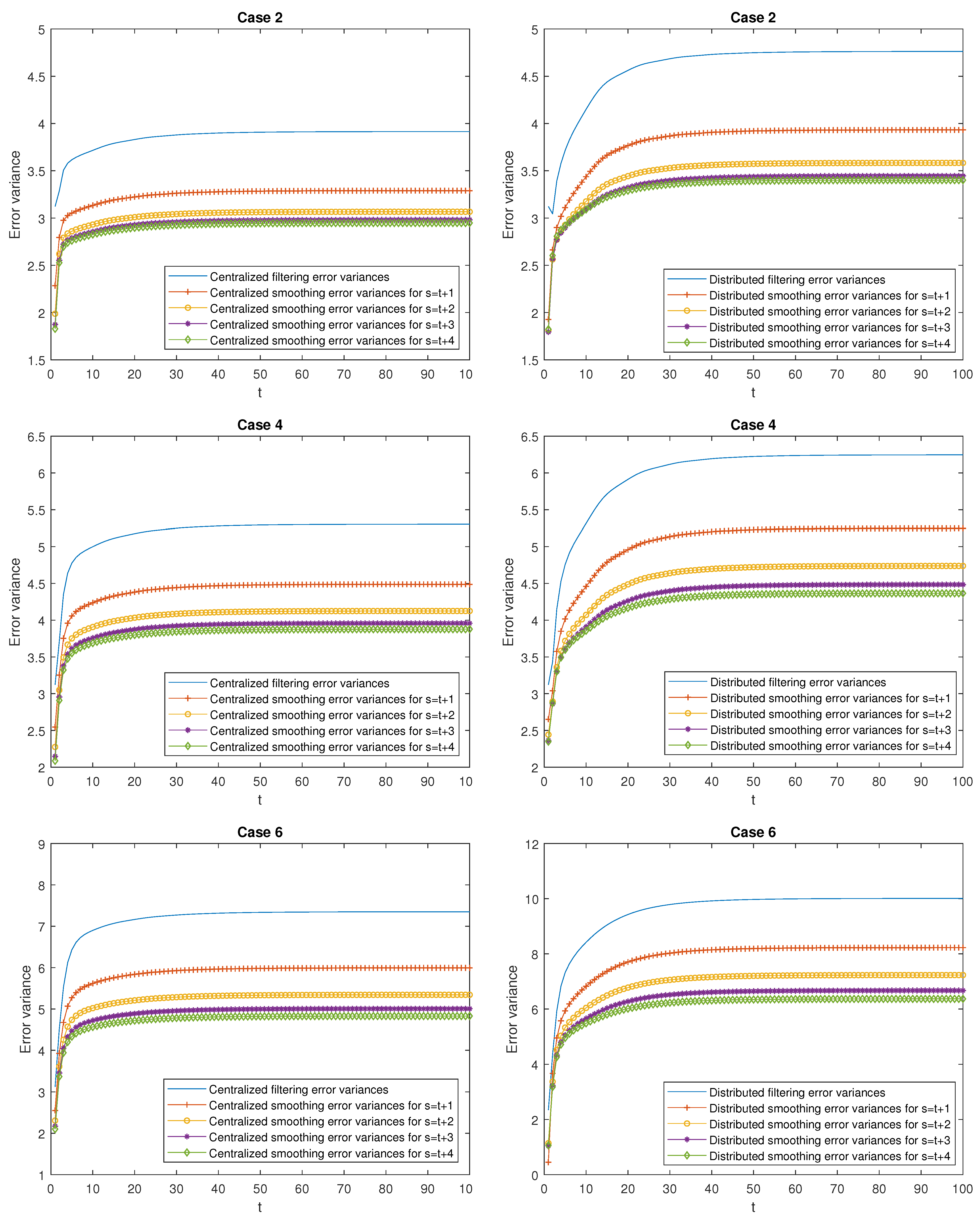
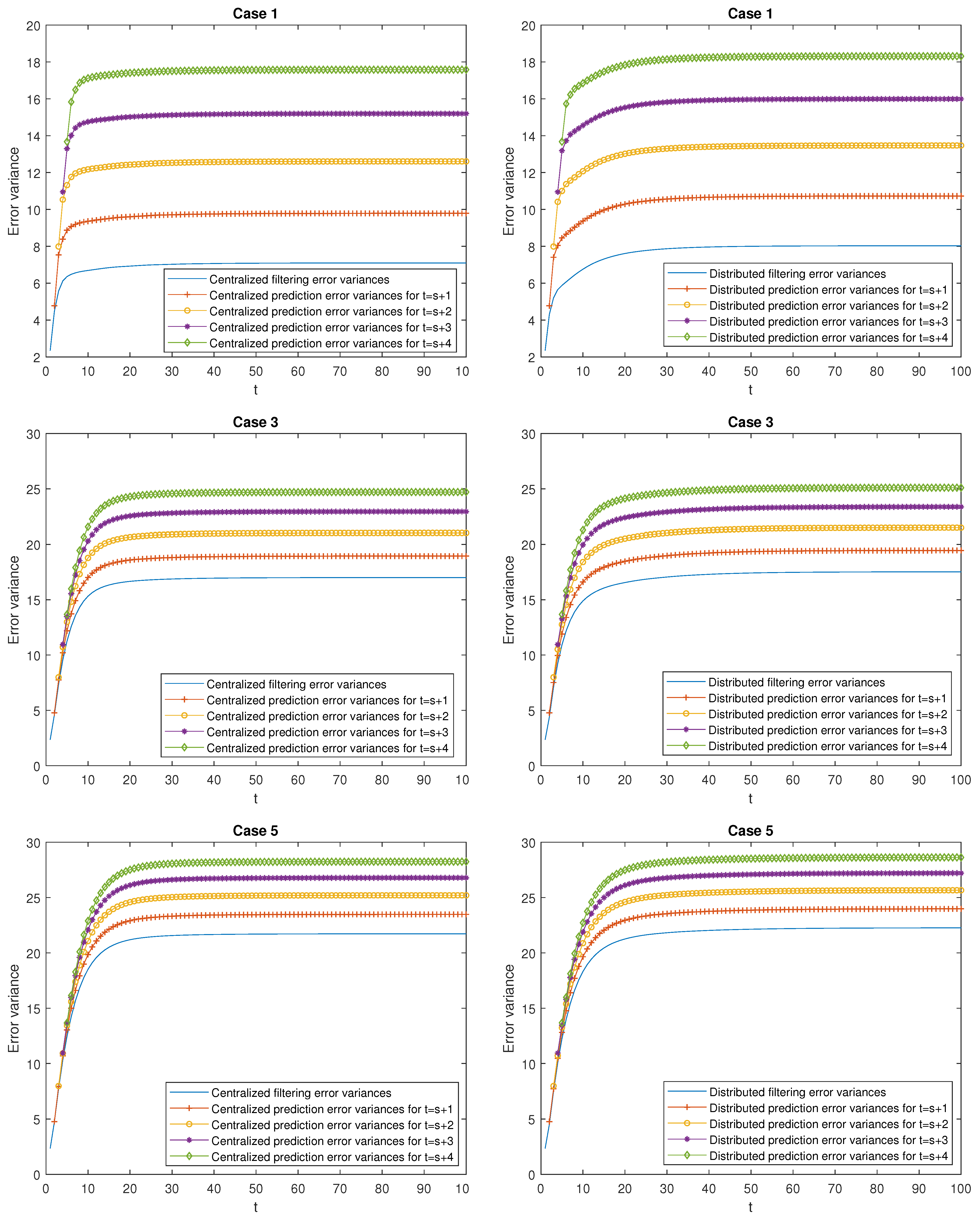
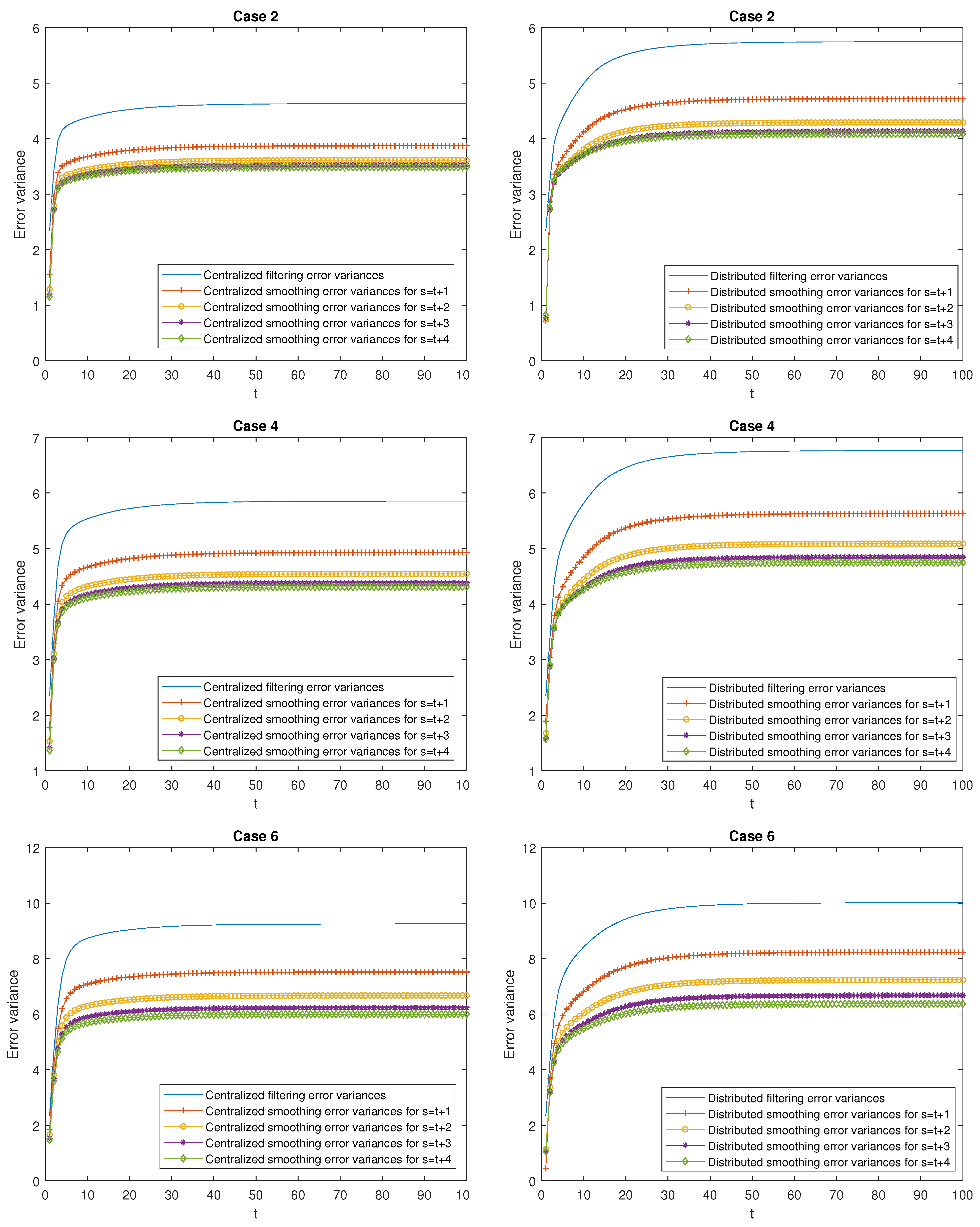
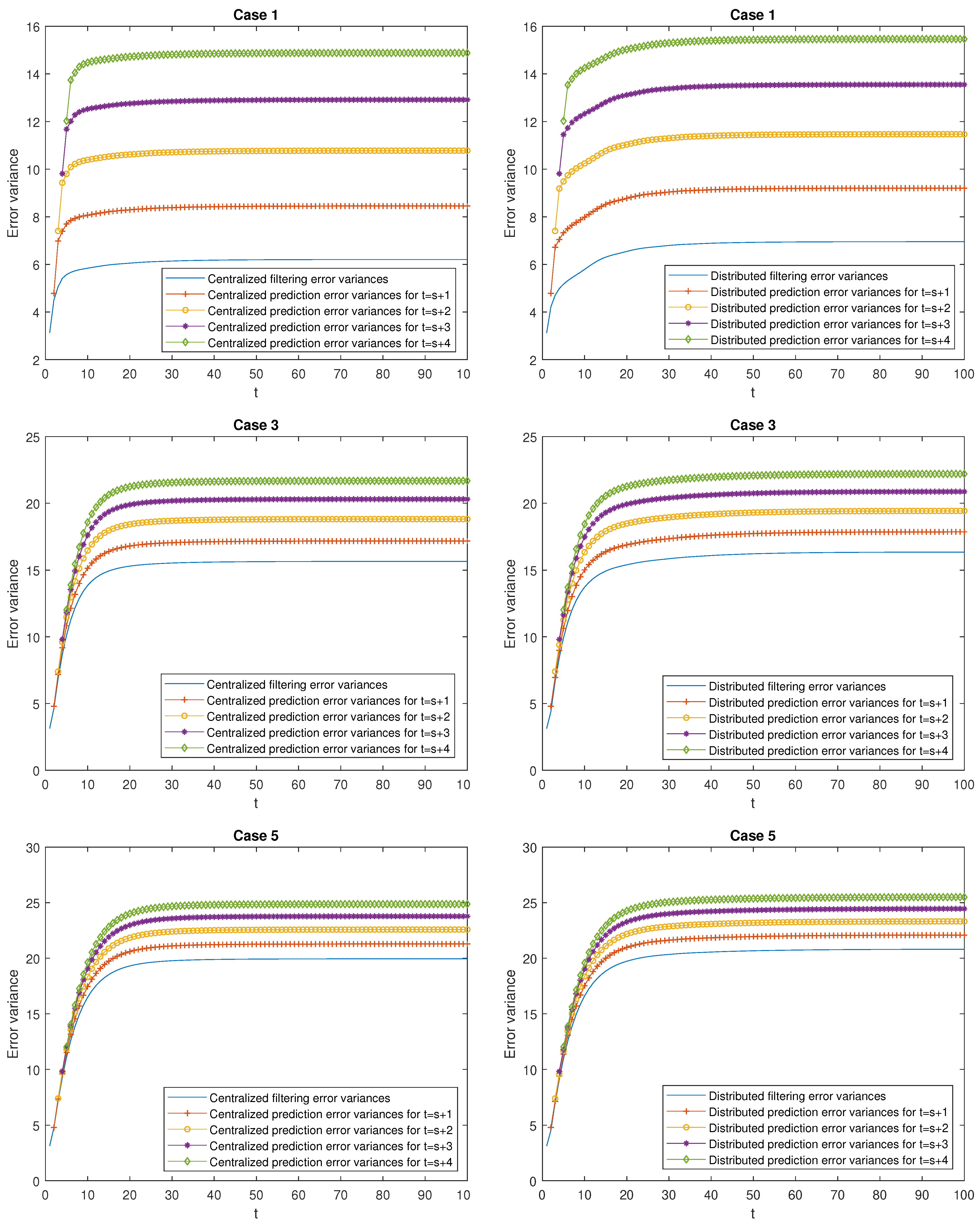
  • Better performance of the centralized estimators over the distributed ones. Effectively, in Case 1, it can be observed that the mean of the centralized and distributed filtering error variances, M E f and M E f D , takes the values 6.9234 and 7.6676 , respectively, which indicate a better performance of the centralized filters over the distributed ones. The same conclusion can be deduced when comparing the means of the prediction and smoothing error variances at the same stage τ . As an example, observe that the mean of the centralized and distributed prediction error variances for τ = 3 , denoted by M E p , 3 and M E p , 3 D , respectively, take the values 15.0486 and 15.6886 , and the one corresponding to the mean of the centralized and distributed smoothing error variances at stage τ = 2 are given by M E s , 2 = 4.7648 , and M E s , 2 D = 5.1388 . Similar considerations can be made for all the cases.
  • Better performance of the smoothing estimators over the filtering ones and both, in turn, over the prediction ones. Effectively, in Case 1, the following relation is true: M E s , 1 D = 5.9197 < M E f D = 7.6676 < M E p , 1 D = 10.3765 . Similar conclusions are obtained in all the cases and for any τ .
  • Worse performance of the prediction estimators as the stage τ increases (the opposite consideration for the smoothing estimators). As an example, in Case 1, it is observed that M E p , 1 = 9.6168 < M E p , 2 = 12.4458 < M E p , 3 = 15.0486 < M E p , 4 = 17.4433 (for the prediction errors) and M E s , 1 = 5.3697 > M E s , 2 = 4.7648 > M E s , 3 = 4.5051 > M E s , 4 = 4.3921 (for the smoothing errors). Similar considerations can be made for all the cases.
Moreover, the following conclusions can be drawn by comparing Cases 1 and 2 in the delay situation, Cases 3 and 4 in the situation of missing measurements, and Cases 5 and 6 for mixed uncertainties. Specifically:
  • In the delay situation: For Cases 1 and 2, it can be observed that the estimations obtained in Case 2 outperform the ones obtained in Case 1, due to the fact that in this case, the probability that the measurements are updated is greater than that of Case 1.
  • In the situation of missing measurements: For Cases 3 and 4, the probability that the measurements contain only noise is smaller in Case 4 than in Case 3; hence, better estimations are obtained.
  • In the situation of mixed uncertainties: For Cases 5 and 6, better estimations are obtained in Case 6 versus Case 5 since there is a greater probability that the measurements are updated or delayed and a lower probability that they contain only noise.
These same conclusions obtained from Table 2 for the T 1 -proper case can be drawn from Table 3 for the T 2 -proper one.

6.2. Example 2

In this second example, the effectiveness of our method is assessed in a realistic setting where the superiority of the proposed estimators over their counterparts in the quaternion domain under T k -properness conditions is analyzed in the case of a single sensor.
Specifically, we consider the following general equation of motion [21]:
φ t = ϕ and ϕ t = ω
where ω is the input of the system, and φ represents the variable of interest with ϕ indicating its range of change.
Note that the equations given in (29) are applicable in a wide variety of practical situations including bearings-only and rotation tracking. In the case of bearing-only tracking applications, the input typically represents force or acceleration, and in a rotation tracking scenario, it represents the torque or angular acceleration.
Consider the equivalent discrete-time model of (29)
x ( t + 1 ) = 1 Δ T 0 1 x ( t ) + Δ T 2 / 2 Δ T ω ( t ) , t = 1 , , 100 .
with x ( t ) = φ ( t ) , ϕ ( t ) T , and initial condition x ( 0 ) = 0 2 × 1 . Moreover, Δ T = 0.04 denotes the sampling interval, and the input ω ( t ) is a tessarine white noise with real covariance matrix given by
E ω r ( t ) ω r T ( s ) = 3 0 2 0 0 3 0 2 2 0 3 0 0 2 0 3 δ t s
By way of illustration, assume that the measurements available come from one sensor according to the equation (2), where v ( t ) = v 1 ( t ) , v 2 ( t ) T is a tessarine white noise such that v 1 ( t ) and v 2 ( t ) are independent and their associated real covariance matrices are given by
E v m r ( t ) v m r T ( s ) = 6.5 0 0.1 0 0 6.5 0 0.1 0.1 0 6.5 0 0 0.1 0 6.5 δ t s , m = 1 , 2
Moreover, the independent Bernoulli random variables γ j m , ν ( t ) , for j = 1 , 2 , m = 1 , 2 , and ν = r , η , η η , have constant parameters p j m , ν ( t ) = p j m , ν .
In this setting, the comparative analysis is carried under both T k -proper, k = 1 , 2 scenarios, by considering the following Bernoulli parameters:
-
T 1 -proper scenario: p 11 , ν = 0.2 , p 12 , ν = 0.3 , p 21 , ν = 0.4 and p 22 , ν = 0.4 , for all ν = r , η , η η , and
-
T 2 -proper scenario: p 11 , r = p 11 , η = 0.7 and p 11 , η = p 11 , η = 0.3 , p 12 , r = p 12 , η = 0.1 and p 12 , η = p 12 , η = 0.8 , p 21 , r = p 21 , η = 0.2 and p 21 , η = p 21 , η = 0.5 , and p 22 , r = p 22 , η = 0.4 and p 22 , η = p 22 , η = 0.2 .
Then, for each T k -proper scenario, k = 1 , 2 , the T k -proper LS linear estimation error variances P k ( t | s ) are compared with their counterparts in the quaternion domain, i.e., the quaternion strictly linear (QSL) and the quaternion semi-widely linear (QSWL) estimation error variances, denoted by P Q S L ( t | s ) and P Q S W L ( t | s ) , respectively. As a measurement for comparison, we consider the difference between both errors for the prediction and smoothing problems given by the expressions:
-
T 1 -proper scenario: D 1 ( t | s ) = P Q S L ( t | s ) P 1 ( t | s ) .
-
T 2 -proper scenario: D 2 ( t | s ) = P Q S W L ( t | s ) P 2 ( t | s ) .
Figure 5 and Figure 6 display these differences for the variable of interest φ ( t ) in the T 1 and T 2 -proper case, respectively. All the graphics show the superiority of the T k -proper estimators over their counterparts in the quaternion domain. Moreover, in the prediction problem, this superiority is higher as time ahead in the prediction stage is greater, whereas in the smoothing problem, a better performance of the T k -proper estimators is achieved in situations with a lower number of measurements used to estimate the state. Note that similar results are obtained for the component ϕ ( t ) of state vector x ( t ) . These graphs have been omitted to not increase the length of the paper.

7. Discussion

The multisensor fusion prediction and smoothing estimation problems in systems with random sensor delays, missing measurements, and correlated noises have been investigated. As usual, these uncertainties are assumed to be modeled by independent Bernoulli distributed random processes.
Unlike most of the results existing in the literature, the problem has been addressed in the tessarine domain. An extremely interesting characteristic of this type of processing is the possibility to reduce the dimension of the problem when the processes involved are T k -proper. In practice, these properness characteristics can be statistically tested. Then, both distributed and centralized fusion estimation algorithms are proposed under T k -properness conditions, which offer significant computational advantages when compared to their counterparts derived from a real-valued processing.
It should be highlighted that as an alternative to tessarines, some other 4D hypercomplex algebras, such as quaternions, could have been used. The convenience of using a tessarine or quaternion processing depends on the particular property conditions verified by the processes involved. Additionally, in future research, more general structures, such as the generalised Segre’s quaternions, which include tessarines as a particular case, would offer the possibility to choose the best commutative algebra according to its properness characteristics.

Author Contributions

All authors have contributed equally to the work. The functions mainly carried out by each specific author are detailed below. Conceptualization, R.M.F.-A.; formal analysis, J.D.J.-L., R.M.F.-A., J.N.-M. and J.C.R.-M.; methodology, R.M.F.-A. and J.D.J.-L.; investigation, J.D.J.-L., R.M.F.-A., J.N.-M. and J.C.R.-M.; visualization, R.M.F.-A., J.D.J.-L., J.N.-M. and J.C.R.-M.; writing—original draft preparation, R.M.F.-A. and J.D.J.-L.; writing—review and editing, R.M.F.-A., J.D.J.-L., J.N.-M. and J.C.R.-M.; funding acquisition, R.M.F.-A. and J.N.-M.; project administration, R.M.F.-A. and J.N.-M.; software, J.D.J.-L.; supervision, J.N.-M. and J.C.R.-M.; validation, J.N.-M. and J.C.R.-M. All authors have read and agreed to the published version of the manuscript.

Funding

This work has been supported in part by the Project PID2021-124486NB-I00 of the ‘’Plan Estatal de I+D+i, Ministerio de Educación y Ciencia, Spain, the I+D+i Project with reference number 1256911 of ‘Programa Operativo FEDER Andalucía 2014–2020’, Junta de Andalucía, and Project EI-FQM2-2021 of ‘Plan de Apoyo a la Investigación 2021–2022’ from the University of Jaén.

Institutional Review Board Statement

Not applicable.

Informed Consent Statement

Not applicable.

Data Availability Statement

Not applicable.

Conflicts of Interest

The authors declare no conflict of interest. The funders had no role in the design of the study: in the collection, analyses, or interpretation of data; in the writing of the manuscript, or in the decision to publish the results.

Appendix A. Proof of Theorem 2

Based on an innovation approach, the optimal LS linear predictor, x ¯ ^ ( i ) ( t | s ) , for each sensor i = 1 , , R , can be obtained from the following expression [32]:
x ¯ ^ ( i ) ( t | s ) = l = 1 t Θ ¯ k ( i ) ( t , l ) Ω k ( i ) 1 ( l ) ϵ k ( i ) ( l ) , t > s
where Θ ¯ k ( i ) ( t , l ) = E x ¯ ( t ) ϵ k ( i ) H ( l ) , Ω k ( i ) ( l ) = E ϵ k ( i ) ( l ) ϵ k ( i ) H ( l ) , and the innovations ϵ k ( i ) ( t ) = y k ( i ) ( t ) y ^ k ( i ) ( t | t 1 ) , with y ^ k ( i ) ( t | t 1 ) the local LS linear estimator of y k ( i ) ( t ) based on the set of available measurements y k ( i ) ( 1 ) , , y k ( i ) ( t 1 ) . Then, using the state equation in (3), and taking into account the fact that E u ¯ ( t ) ϵ k ( i ) H ( s ) = 0 4 n × k n , for t > s , the following expression is obtained:
x ¯ ^ ( i ) ( t | s ) = Φ ¯ ( t 1 ) x ¯ ^ ( i ) ( t 1 | s ) , t > s + 1 .
Therefore, Equation (14) is immediately derived by characterizing (A1) for both T k -proper scenarios.
Moreover, from (A1), the following equation is obtained:
x ¯ ˜ ( i ) ( t | s ) = Φ ¯ ( t 1 ) x ¯ ˜ ( i ) ( t 1 | s ) + u ¯ ( t 1 ) , t > s + 1 ,
where x ¯ ˜ ( i ) ( t | s ) = x ¯ ( t ) x ¯ ^ ( i ) ( t | s ) and x ¯ ˜ ( i ) ( t 1 | s ) = x ¯ ( t 1 ) x ¯ ^ ( i ) ( t 1 | s ) . Hence, Equation (15) is deduced by characterizing (A2) for both T k -proper scenarios.

Appendix B. Proof of Theorem 3

Similar to the Proof of Theorem 2 given in Appendix A, the optimal LS linear smoother, x ¯ ^ ( i ) ( t | s ) , can be expressed as follows [2]:
x ¯ ^ ( i ) ( t | s ) = l = 1 s Θ ¯ k ( i ) ( t , l ) Ω k ( i ) 1 ( l ) ϵ k ( i ) ( l ) , s > t ,
and hence, the following recursive expression is easily derived:
x ¯ ^ ( i ) ( t | s ) = x ¯ ^ ( i ) ( t | s 1 ) + L ¯ k ( i ) ( t , s ) ϵ k ( i ) ( s ) , s > t .
Then, Equation (16) is easily derived from (A4), and taking into account the characteristics of both T k -proper scenarios.
Analogously, the optimal LS linear filter, x ¯ ^ ( i ) ( s | s ) , and the one-stage predictor, x ¯ ^ ( i ) ( s | s 1 ) , admit the following expressions:
x ¯ ^ ( i ) ( s | s ) = x ¯ ^ ( i ) ( s | s 1 ) + L ¯ k ( i ) ( s ) ϵ k ( i ) ( s ) ,
and
x ¯ ^ ( i ) ( s | s 1 ) = Φ ¯ ( s 1 ) x ¯ ^ ( i ) ( s 1 | s 1 ) + H ¯ k ( i ) ( s 1 ) ϵ k ( i ) ( s 1 ) ,
respectively, where L ¯ k ( i ) ( s ) = Θ ¯ k ( i ) ( s ) Ω k ( i ) 1 ( s ) , with Θ ¯ k ( i ) ( s ) = Θ ¯ k ( i ) ( s , s ) , and H ¯ k ( i ) ( s 1 ) = S ¯ ( i ) ( s 1 ) Π k 1 γ 2 ( i ) H ( s 1 ) Ω k ( i ) 1 ( s 1 ) .
Now, from (6) and (9), we have
Θ ¯ k ( i ) ( t , s ) = E x ¯ ( t ) x ¯ ˜ ( i ) H ( s | s 1 ) Π k γ 1 ( i ) H ( s ) + E ¯ k ( i ) ( t , s 1 ) Θ ¯ k ( i ) ( t , s 1 ) G ¯ k ( i ) H ( s 1 ) Π k γ 2 ( i ) H ( s ) ,
where E ¯ k ( i ) ( t , s 1 ) = E x ¯ ( t ) x ¯ ˜ ( i ) H ( s 1 | s 1 ) , and G ¯ k ( i ) ( s 1 ) = R ¯ ( i ) ( s 1 ) Π k 1 γ 2 ( i ) H ( s 1 ) Ω k ( i ) 1 ( s 1 ) . Thus, from (3), (A5), and (A6), and reordering terms, Equation (17) is derived by using the characteristics of both T k -proper scenarios on the resulting expression. Its initial condition is immediately deduced from its definition.
In a similar way, from (3), (A5), and (A6), the expression (18) is directly obtained by virtue of the T k -properness conditions.
Finally, the recursive formula (19) for the pseudo covariance matrix of the smoothing errors P k ( i ) ( t | s ) is easily derived from (16).

Appendix C. Proof of Theorem 5

From (A1), the pseudo-cross-covariance matrix K ¯ ( i j ) ( t , s ) = E x ^ ( i ) ( t | s ) x ^ ( j ) H ( t | s ) , for t > s + 1 , takes the form
K ¯ ( i j ) ( t , s ) = Φ ¯ ( t 1 ) K ¯ ( i j ) ( t 1 , s ) Φ ¯ H ( t 1 ) , t > s + 1 .
Hence, by characterizing this expression for both T k -proper scenarios, Equation (20) can be deduced.

Appendix D. Proof of Theorem 6

From (16), K ¯ ( i j ) ( t , s ) E x ^ ( i ) ( t | s ) x ^ ( j ) H ( t | s ) , for s > t , can be expressed as follows:
K ¯ ( i j ) ( t , s ) = K ¯ ( i j ) ( t , s 1 ) + N ¯ k ( i j ) ( t , s ) L ¯ k ( j ) H ( t , s ) + L ¯ k ( i ) ( t , s ) L ¯ k ( j i ) H ( t , s ) , s > t ,
where N ¯ k ( i j ) ( t , s ) = E x ¯ ^ ( i ) ( t | s ) ϵ k ( i ) H ( s ) = L ¯ k ( i j ) ( t , s ) + L ¯ k ( i ) ( t , s ) M k ( i j ) ( s ) , with L ¯ k ( i j ) ( t , s ) = E x ¯ ^ ( i ) ( t | s 1 ) ϵ k ( i ) H ( s ) . Then, Equation (21) is easily derived by characterizing (A7) for both T k -proper scenarios. The initial condition is directly obtained from its definition.
Next, from (9), the following expression for L ¯ k ( i j ) ( t , s ) , with s > t , is obtained:
L ¯ k ( i j ) ( t , s ) = E x ¯ ^ ( i ) ( t | s 1 ) y k ( j ) H ( s ) E x ¯ ^ ( i ) ( t | s 1 ) x ¯ ^ ( j ) H ( s | s 1 ) Π k γ 1 ( j ) H ( s ) O ¯ ( i j ) ( t , s 1 ) Π k γ 2 ( j ) H ( s ) N ¯ k ( i j ) ( t , s 1 ) G ¯ k ( j ) H ( s 1 ) Π k γ 2 ( j ) H ( s ) , s > t ,
with O ¯ ( i j ) ( t , s ) = E x ¯ ^ ( i ) ( t | s ) x ¯ ^ ( j ) H ( s | s ) . Now, by using (6), the hypotheses on the model, and Equations (A3) and (A6), the following equation can be obtained:
E x ¯ ^ ( i ) ( t | s 1 ) y k ( j ) H ( s ) = O ¯ ( i i ) ( t , s 1 ) A ¯ k ( j ) H ( s 1 ) + Θ ¯ k ( i ) ( t , s 1 ) H ¯ k ( i ) H ( s 1 ) Π k γ 1 ( j ) H ( s ) + L ¯ k ( i ) ( t , s 1 ) Θ ¯ v k ( j i ) H ( s 1 ) Π k γ 2 ( j ) H ( s ) , E x ¯ ^ ( i ) ( t | s 1 ) x ¯ ^ ( j ) H ( s | s 1 ) = O ¯ ( i j ) ( t , s 1 ) Φ ¯ H ( s 1 ) + N ¯ k ( i j ) ( t , s 1 ) H ¯ k ( j ) H ( s 1 ) ,
where A ¯ k ( j ) ( s 1 ) = Π k γ 1 ( j ) ( s ) Φ ¯ ( s 1 ) + Π k γ 2 ( j ) ( s ) . Then, by substituting (A9) in (A8), reordering terms, and taking into account the characteristics of the T k -proper scenarios, Equation (22) is deduced. Its initial condition is determined by its proper definition.
Finally, to derive Equation (23), the following expression will be used,
x ¯ ^ ( j ) ( s | s ) = Φ ¯ ( s 1 ) x ¯ ^ ( j ) ( s 1 | s 1 ) + H ¯ k ( j ) ( s 1 ) ϵ k ( j ) ( s 1 ) + L ¯ k ( j ) ( s ) ϵ k ( j ) ( s ) ,
immediately obtained from (A5) and (A6). Then, by using the definition of O ¯ ( i j ) ( t , s ) , (A4) and (A10), reordering terms in the resultant expression, and applying the characterization of both T k -proper scenarios, Equation (23) can be deduced. From its definition, the initial condition is established.

References

  1. Kurkin, A.A.; Tyugin, D.Y.; Kuzin, V.D.; Chernov, A.G.; Makarov, V.S.; Beresnev, P.O.; Filatov, V.I.; Zeziulin, D.V. Autonomous mobile robotic system for environment monitoring in a coastal zone. Procedia Comput. Sci. 2017, 103, 459–465. [Google Scholar] [CrossRef]
  2. Hsu, Y.-L.; Chou, P.-H.; Chang, H.-C.; Lin, S.-L.; Yang, S.-C.; Su, H.-Y.; Chang, C.-C.; Cheng, Y.-S.; Kuo, Y.-C. Design and Implementation of a Smart Home System Using Multisensor Data Fusion Technology. Sensors 2017, 17, 1631. [Google Scholar] [CrossRef]
  3. Gao, B.; Hu, G.; Gao, S.; Zhong, Y.; Gu, C.; Beresnev, P.O.; Filatov, V.I.; Zeziulin, D.V. Multi-sensor optimal data fusion for INS/GNSS/CNS integration based on unscented Kalman filter. Int. J. Control Autom. Syst. 2018, 16, 129–140. [Google Scholar] [CrossRef]
  4. Huang, S.; Chou, P.; Jin, X.; Zhang, Y.; Jiang, Q.; Yao, S. Multi-Sensor image fusion using optimized support vector machine and multiscale weighted principal component analysis. Electronics 2020, 9, 1531. [Google Scholar] [CrossRef]
  5. Gao, B.; Hu, G.; Zhong, Y.; Zhu, X. Cubature rule-based distributed optimal fusion with identification and prediction of kinematic model error for integrated UAV navigation. Aerosp. Sci. Technol. 2021, 109, 1106447. [Google Scholar] [CrossRef]
  6. Yukun, C.; Xicai, S.; Zhigang, L. Research on Kalman-filter based multisensor data fusion. J. Syst. Eng. Electron. 2007, 18, 497–502. [Google Scholar] [CrossRef]
  7. Ding, F. Combined state and least squares parameter estimation algorithms for dynamic systems. Appl. Math. Model. 2014, 38, 403. [Google Scholar] [CrossRef]
  8. Shenglun, Y.; Mattia, Z. Robust Kalman Filtering under Model Uncertainty: The Case of Degenerate Densities. IEEE Trans. Automat. Contr. 2021. [Google Scholar] [CrossRef]
  9. Ma, J.; Sun, S. Centralized fusion estimators for multisensor systems with random sensor delays, multiple packet dropouts and uncertain observations. IEEE Sens. J. 2013, 13, 1228–1235. [Google Scholar] [CrossRef]
  10. Chen, D.; Xu, L. Optimal filtering with finite-step autocorrelated process noises, random one-step sensor delay and missing measurements. Commun. Nonlinear Sci. Numer. Simul. 2016, 32, 211–224. [Google Scholar] [CrossRef]
  11. Liu, W.-Q.; Wang, X.-M.; Deng, Z.-L. Robust centralized and weighted measurement fusion Kalman estimators for uncertain multisensor systems with linearly correlated white noises. Inf. Fusion 2017, 35, 11–25. [Google Scholar] [CrossRef]
  12. Lin, H.; Sun, S. Distributed fusion estimator for multi-sensor asynchronous sampling systems with missing measurements. IET Signal Process. 2016, 10, 724–731. [Google Scholar] [CrossRef]
  13. Tian, T.; Sun, S.; Li, N. Multi-sensor information fusion estimators for stochastic uncertain systems with correlated noises. Inf. Fusion 2016, 27, 126–137. [Google Scholar] [CrossRef]
  14. Xing, Z.; Xia, Y.; Yan, L.; Lu, K.; Gong, Q. Multisensor distributed weighted Kalman filter fusion with network delays, stochastic uncertainties, autocorrelated, and cross-correlated noises. IEEE Trans. Syst. Man Cyber. Syst. 2018, 48, 716–726. [Google Scholar] [CrossRef]
  15. Zhang, J.; Gao, S.; Li, G.; Xia, J.; Qi, X.; Gao, B. Distributed recursive filtering for multi-sensor networked systems with multi-step sensor delays, missing measurements and correlated noise. Signal Process. 2021, 181, 107868. [Google Scholar] [CrossRef]
  16. Yuan, X.; Yu, S.; Zhang, S.; Wang, G.; Liu, S. Quaternion-Based Unscented Kalman Filter for Accurate Indoor Heading Estimation Using Wearable Multi-Sensor System. Sensors 2015, 15, 10872–10890. [Google Scholar] [CrossRef]
  17. Talebi, S.; Kanna, S.; Mandic, D. A distributed quaternion Kalman filter with applications to smart grid and target tracking. IEEE Trans. Signal Inf. Process. Netw. 2016, 2, 477–488. [Google Scholar]
  18. Tannous, H.; Istrate, D.; Benlarbi-Delai, A.; Sarrazin, J.; Gamet, D.; Ho Ba Tho, M.C.; Dao, T.T. A new multi-sensor fusion scheme to improve the accuracy of knee flexion kinematics for functional rehabilitation movements. J. Sens. 2016, 16, 1914. [Google Scholar] [CrossRef] [Green Version]
  19. Navarro-Moreno, J.; Fernández-Alcalá, R.M.; Jiménez López, J.D.; Ruiz-Molina, J.C. Widely linear estimation for multisensor quaternion systems with mixed uncertainties in the observations. J. Frankl. Inst. 2019, 356, 3115–3138. [Google Scholar] [CrossRef]
  20. Wu, J.; Zhou, Z.; Fourati, H.; Li, R.; Liu, M. Generalized linear quaternion complementary filter for attitude estimation from multi-sensor observations: An optimization approach. IEEE Trans. Autom. Sci. Eng. 2019, 16, 1330–1343. [Google Scholar] [CrossRef]
  21. Talebi, S.P.; Werner, S.; Mandic, D.P. Quaternion-valued distributed filtering and control. IEEE Trans. Autom. Control. 2020, 65, 4246–4256. [Google Scholar] [CrossRef]
  22. Fernández-Alcalá, R.M.; Navarro-Moreno, J.; Ruiz-Molina, J.C. T-proper hypercomplex centralized fusion estimation for randomly multiple sensor delays systems with correlated noises. Sensors 2021, 21, 5729. [Google Scholar] [CrossRef]
  23. Jiménez-López, J.D.; Fernández-Alcalá, R.M.; Navarro-Moreno, J.; Ruiz-Molina, J.C. The distributed and centralized fusion filtering problems of tessarine signals from multi-sensor randomly delayed and missing observations under Tk-properness conditions. Mathematics 2021, 9, 2961. [Google Scholar] [CrossRef]
  24. Zanetti de Castro, F.; Eduardo Valle, M. A broad class of discrete-time hypercomplex-valued Hopfield neural networks. Neural Netw. 2020, 122, 54–67. [Google Scholar] [CrossRef] [PubMed] [Green Version]
  25. Alfsmann, D. On families of 2N-dimensional hypercomplex algebras suitable for digital signal processing. In Proceedings of the 14th European Signal Processing Conference, 14th European Signal Processing Conference (EUSIPCO 2006), Florence, Italy, 4–8 September 2006; pp. 1–4. [Google Scholar]
  26. Alfsmann, D.; Göckler, H.G.; Sangwine, S.J.; Ell, T.A. Hypercomplex algebras in digital signal processing: Benefits and drawbacks. In Proceedings of the 15th European Signal Processing Conference, Poznan, Poland, 3–7 September 2007; pp. 1322–1326. [Google Scholar]
  27. Hahn, S.L.; Snopek, K.M. Complex and Hypercomplex Analytic Signals: Theory and Applications; Artech House: Norwood, MA, USA, 2016. [Google Scholar]
  28. Catoni, F.; Boccaletti, D.; Cannata, R.; Catoni, V.; Nichelatti, E.; Zampetti, P. The Mathematics of Minkowski Space-Time: With an Introduction to Commutative Hypercomplex Numbers; Birkhaüser Verlag: Basel, Switzerland, 2008. [Google Scholar]
  29. Navarro-Moreno, J.; Ruiz-Molina, J.C. Wide-sense Markov signals on the tessarine domain. A study under properness conditions. Signal Process. 2021, 183, 108022. [Google Scholar] [CrossRef]
  30. Nitta, T.; Kobayashi, M.; Mandic, D.P. Hypercomplex widely linear estimation through the lens of underpinning geometry. IEEE Trans. Signal Process. 2019, 67, 3985–3994. [Google Scholar] [CrossRef]
  31. Grassucci, E.; Comminiello, D.; Uncini, A. An information-theoretic perspective on proper quaternion variational autoencoders. Entropy 2021, 23, 856. [Google Scholar] [CrossRef]
  32. Navarro-Moreno, J.; Fernández-Alcalá, R.M.; Jiménez-López, J.D.; Ruiz-Molina, J.C. Tessarine signal processing under the T-properness condition. J. Frankl. Inst. 2020, 357, 10100. [Google Scholar] [CrossRef]
Figure 1. Filtering and prediction error variances in the T 1 -proper scenario for Cases 1, 3, and 5 computed by using the centralized fusion algorithm (on the left) and the distributed algorithm (on the right).
Mathematics 10 02495 g001
Figure 2. Filtering and smoothing error variances in the T 1 -proper scenario for Cases 2, 4, and 6 computed by using the centralized fusion algorithm (on the left) and the distributed algorithm (on the right).
Mathematics 10 02495 g002
Figure 3. Filtering and prediction error variances in the T 2 -proper scenario for Cases 1, 3, and 5 computed by using the centralized fusion algorithm (on the left) and the distributed algorithm (on the right).
Mathematics 10 02495 g003
Figure 4. Filtering and smoothing error variances in the T 1 -proper scenario for Cases 2, 4, and 6 computed by using the centralized fusion algorithm (on the left) and the distributed algorithm (on the right).
Mathematics 10 02495 g004
Figure 5. Difference between QSL and T 1 -proper error variances for the prediction (on the left) and smoothing (on the right) problems in the T 1 -proper scenario.
Mathematics 10 02495 g005
Figure 6. Difference between QSWL and T 2 -proper error variances for the prediction (on the left) and the smoothing (on the right) problems in the T 2 -proper scenario.
Mathematics 10 02495 g006
Table 1. Expressions for filtering, prediction, and smoothing mean square errors.
Fusion MethodFilteringPredictionSmoothing
Centralized M E f = 1 100 t = 1 100 P T k ( t | t ) M E p , τ = 1 100 τ t = 1 100 τ P T k ( t + τ | t ) M E s , τ = 1 100 t = 1 100 P T k ( t | t + τ )
Distributed M E f D = 1 100 t = 1 100 P D T k ( t | t ) M E p , τ D = 1 100 τ t = 1 100 τ P D T k ( t + τ | t ) M E s , τ D = 1 100 t = 1 100 P D T k ( t | t + τ )
Table 2. Filtering, prediction, and smoothing mean square errors in the T 1 -proper scenario.
Cases

Filtering
ME f
ME f D
Prediction:
ME p , τ
ME p , τ D
Smoothing:
ME s , τ
ME s , τ D
τ = 1 τ = 2 τ = 3 τ = 4 τ = 1 τ = 2 τ = 3 τ = 4
16.9234
7.6676
9.6168
10.3765
12.4458
13.1431
15.0486
15.6886
17.4433
18.0306
5.3697
5.9197
4.7648
5.1388
4.5051
4.7790
4.3921
4.6328
24.5390
5.5281
6.7719
7.8469
9.8292
10.8171
12.6421
13.5498
15.2299
16.0640
3.7946
4.5354
3.5424
4.1401
3.4435
3.9973
3.4212
3.9622
316.2548
16.5213
18.2474
18.5119
20.3810
20.6221
22.3444
22.5641
24.1511
24.3512
14.9311
15.1552
13.9736
14.1378
13.2796
13.3827
12.7753
12.8245
45.7176
6.4844
7.9889
8.8057
10.9485
11.7014
13.6715
14.3629
16.1767
16.8116
4.8191
5.4013
4.4473
4.8981
4.2898
4.6787
4.2218
4.5968
520.5823
20.9046
22.4152
22.7121
24.2120
24.4833
25.8656
26.1134
27.3876
27.6139
19.1857
19.5125
18.1108
18.4190
17.2780
17.5536
16.6324
16.8704
68.9821
9.5247
11.5869
12.0809
14.2575
14.7101
16.7147
17.1292
18.9754
19.3550
7.3064
7.7961
6.4887
6.8709
6.0641
6.3559
5.8423
6.0840
Table 3. Filtering, prediction, and smoothing mean square errors in the T 2 -proper scenario.
Cases

Filtering
ME f
ME f D
Prediction:
ME p , τ
ME p , τ D
Smoothing:
ME s , τ
ME s , τ D
τ = 1 τ = 2 τ = 3 τ = 4 τ = 1 τ = 2 τ = 3 τ = 4
16.0702
6.6500
8.3156
8.9052
10.6490
11.1900
12.7959
13.2922
14.7711
15.2263
4.7329
5.1555
4.1974
4.4732
3.9544
4.1470
3.8409
4.0052
23.8564
4.6005
5.6914
6.5058
8.2355
8.9830
10.5761
11.2629
12.7295
13.3605
3.2399
3.7966
3.0210
3.4710
2.9380
3.3482
2.9049
3.3127
314.9522
15.3920
16.5263
16.9481
18.1980
18.5837
19.7363
20.0890
21.1520
21.4744
13.8800
14.3013
13.0793
13.4627
12.4797
12.8189
12.0298
12.3261
45.1916
5.9890
7.0810
7.9173
9.5134
10.2815
11.7514
12.4568
13.8103
14.4581
4.3965
5.0333
4.0439
4.5557
3.8817
4.3248
3.8049
4.2216
518.7493
19.4711
20.1627
20.8326
21.5402
22.1542
22.8080
23.3709
23.9750
24.4909
17.6607
18.4132
16.8025
17.5593
16.1205
16.8643
15.5780
16.2995
67.1621
7.9999
9.3053
10.1092
11.5591
12.2969
13.6328
14.3097
15.5406
16.1617
5.8434
6.5764
5.2147
5.8134
4.8912
5.3839
4.7212
5.1533
Publisher’s Note: MDPI stays neutral with regard to jurisdictional claims in published maps and institutional affiliations.

