Neural Network-Based Approximation Model for Perturbed Orbit Rendezvous

Abstract

An approximation of orbit rendezvous is usually used in the global optimization of multi-target rendezvous missions, which can greatly affect the efficiency of optimization process. A fast neural network-based surrogate model is proposed to approximate the optimal velocity increment of perturbed orbit rendezvous in low Earth orbits. According to a dynamic analysis, the initial and target orbits together with the flight time are transformed into a nine-dimensional normalized vector that is used as the input layer of the neural network. An existing approximation method is introduced to quickly generate the training data. In simulations, different numbers of layer nodes and hidden layers are tested to choose the best parameters. The proposed neural network model demonstrates high precision and high efficiency compared with previous approximation methods and neural network models. The mean relative error is less than 1%. Finally, a case of an optimization of a multi-target rendezvous mission is tested to prove the potential application of the neural network model.

1. Introduction

The fast approximation of orbit rendezvous is a basis for the global optimization of a multi-target rendezvous mission [1]. Due to the drift of the right ascension of the ascending node (RAAN) and argument of perigee [2], the rendezvous velocity increment is closely related to the flight time for perturbed orbit rendezvous in low Earth orbits (LEOs), which makes it difficult to obtain an analytical solution. Numerical methods based on evolutionary algorithms can obtain a high-precision solution, but applying them for the global optimization of a multi-target rendezvous sequence is time-consuming [3,4] because the global search needs to evaluate the velocity increments required for orbit transfers between the different targets at different times for many instances to find the global optimal order and arrival time of each target.

To obtain efficient methods that quickly calculate the optimal velocity increment, several studies have focused on analytical methods based on dynamic approximations. A simple strategy is to calculate the orbit differences between the initial and target orbits and add them to the velocity increment separately [5,6]. It is fast enough, but cannot deal with the coupling terms between the different components of the orbit elements. As differences in the semi-major axis and inclination may cause the RAAN to drift due to perturbations, it can be used to indirectly change the RAAN instead of a normal impulse maneuver. Cerf [7] proposed a traversal method to search for the optimal RAAN drift rate to minimize the total impulses. Huang [8,9] established an equal constraint optimization model of different impulse components and derived an extremality condition based on the minimum principle. Shen [10] and Chen [11] separately proposed similar methods by rewriting the objective function to obtain the analytical expression of the optimal solution.

With the development of artificial neural networks [12,13,14], several studies have employed neural networks to approximate the solution of complex dynamic equations. Li [15] proposed a surrogate model of low-thrust transfer between asteroids in deep space. Zhu [16,17] also studied the application of artificial neural networks in low-thrust and impulsive orbit transfers. Due to the effect of perturbations on the orbit elements in low Earth orbits, it is more difficult to find all the features that determine the optimal velocity increment of the rendezvous. In [15,16], the residuals of the neural networks for transfers in deep space were less than 1%. By contrast, in [17], the residual of the neural network for perturbed rendezvous with a similar structure was more than 2%. Moreover, in [17], multiple man-made combinations of characteristic parameters were tested to find the optimal input layer of the neural network for perturbed orbit rendezvous. However, a few of the candidate parameters lacked physical meanings and the orbit rendezvous was divided into three types corresponding with three different neural networks to be trained, which made the process more time-consuming. Therefore, we focused on a neural network structure that precisely reflected the optimization of orbit rendezvous using the fewest parameters.

The major contribution of this study is the proposition of a novel neural network model for the approximation of long-duration perturbed orbit rendezvous. According to the existing analytical methods, the feature vector that completely determines the optimal velocity increment was exacted and normalized to be used as the input layer. The efficiency of the training data generation processes was also improved. The simulation results indicated that the relative error of the neural network was less than 1% and the calculation time was much less. It can be reasonably applied to the global optimization of multi-target rendezvous sequences.

2. Problem Description of Orbit Rendezvous

In this study, we addressed time-fixed impulsive orbit rendezvous in low Earth orbits with small eccentricities. The spacecraft was deemed to be in an initial orbit and needed to transfer to a given target orbit. The rendezvous time and flight time were fixed. Thus, the optimal velocity increment was the minimum summary of impulses that transferred the spacecraft to the target orbit under the gravity of the Earth and other perturbations. The dynamics equations can be described as follows [8]:

$$\begin{array}{l}\dot{r}=v\\ \dot{v}=-\frac{\mu }{r^3}r+a_p\end{array}$$

(1)

where $r$ and $v$ are the position and velocity of the spacecraft, respectively; $r$ is the magnitude of $r$; $\mu$ is the gravity constant of the Earth; and $a_p$ is the acceleration of perturbations, which included the non-sphere perturbation of the Earth, the gravities of the sun and the moon, solar radial pressure, and the drag of the atmosphere [2].

The model of the impulsive maneuver was expressed as:

$$\begin{array}{l}r(t_m{}^{+})=r(t_m{}^{-})\\ v(t_m{}^{+})=v(t_m{}^{-})+\Delta v\end{array}$$

(2)

where $t_m{}^{-}$ and $t_m{}^{+}$ are the instantaneous times before and after the maneuver, respectively, and $\Delta v$ is the vector of impulse. Assuming that $\{\Delta v_i\},i=1,2\dots n$ is the sequence of impulses that ensures that the spacecraft rendezvous with a target orbit, the optimization problem is:

$$\begin{array}{l}\min J={\displaystyle \sum _{i=1}^n\left|\Delta v_i\right|}\\ s.t.r(t_f)=r_f\\ v(t_f)=v_f\end{array}$$

(3)

where $t_f$ is the rendezvous time; $r_f$ and $v_f$ are the position and velocity of the target orbit, respectively; and n is the number of impulses.

Equation (3) is a non-linear optimization model and evolutionary algorithms are always required to obtain a high-precision solution. When searching for the best path and rendezvous times of each target in a multi-target sequence, the global optimization process needs to frequently evaluate the velocity increments of the transfers between the different targets with different flight times, which is extremely time-consuming. Most existing studies have employed different forms of approximation to improve the efficiency [5,6,7,8,11]. However, such a problem still lacks a solution that is fast enough for global optimization. In this study, we propose a new artificial neural network approach to approximate the optimal velocity increment.

3. Methodology

In this section, the semi-analytical approximation method in [8] was reviewed first. Based on this method, the features that fully determined the velocity increment were extracted and validated by the sampling data of different orbit elements and transfer durations. The feature vector was then employed as the input layer of a multi-layer neural network. Meanwhile, the numerical high-precision solution in [9] was applied to generate the sampling data for the training and validation. The process was as follows.

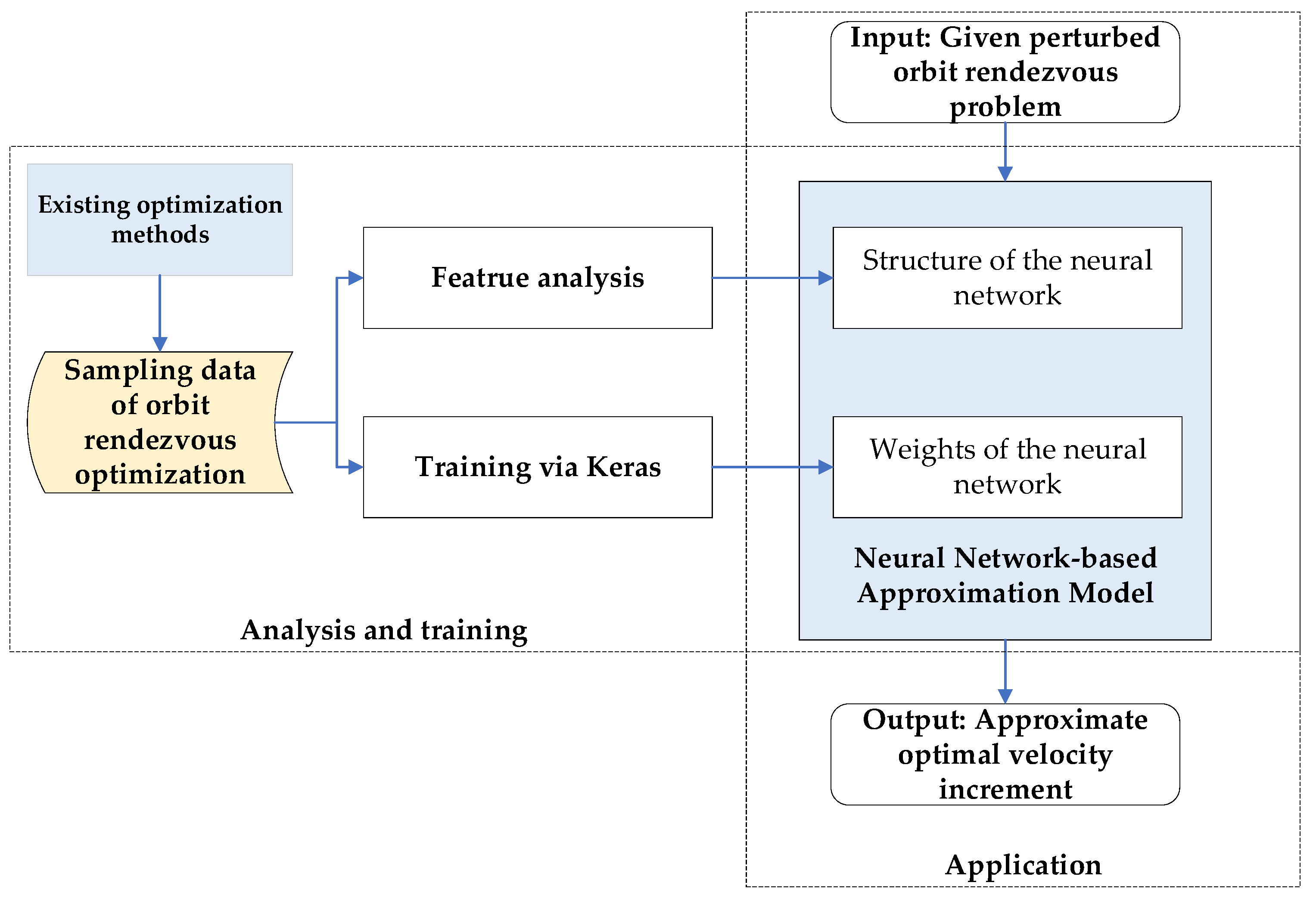
3.1. Approximation Method of the Perturbed Orbit Rendezvous Problem

To quickly evaluate the optimal velocity increment, Huang [8] proposed a semi-analytical model that considered both efficiency and precision in which the analytical dynamic equations of J₂ perturbation were used and the changes in the orbit elements by maneuvers were set as unknown parameters. We assumed that $\Delta a_0,\Delta i_0\mathrm{and}\Delta {\mathsf{\Omega }}_0$ were the differences of the semi-major axis, inclination, and RAAN between the initial and target orbits. $\Delta a_1$, $\Delta i_1$, and $\Delta {\mathsf{\Omega }}_1$ then denoted the changes in the semi-major axis, inclination, and RAAN caused by the impulses at the beginning of the transfer. $\Delta a_2$, $\Delta i_2$, and $\Delta {\mathsf{\Omega }}_2$ denoted the changes in semi-major axis, inclination, and RAAN caused by the impulses at the end of the transfer. Thus, the equality constraint optimization model was obtained as:

$$\begin{array}{l}\min \Delta v=\sqrt{{(\frac{\Delta a_1}{2a_0})}^2+{(\Delta i_1)}^2+{(\frac{\Delta {\mathsf{\Omega }}_1}{\sin i_0})}^2}+\sqrt{{(\frac{\Delta a_2}{2a_0})}^2+{(\Delta i_2)}^2+{(\frac{\Delta {\mathsf{\Omega }}_2}{\sin i_0})}^2}\\ g.t.g_1\triangleq \Delta a_1+\Delta a_2=\Delta a_0\\ g_2\triangleq \Delta i_1+\Delta i_2=\Delta i_0\\ g_3\triangleq \Delta {\mathsf{\Omega }}_1+\Delta {\mathsf{\Omega }}_2+\Delta \dot{\mathsf{\Omega }}\Delta t=\Delta {\mathsf{\Omega }}_0\end{array}$$

(4)

where $\Delta a_1$, $\Delta i_1$, $\Delta {\mathsf{\Omega }}_1$, $\Delta a_2$, $\Delta i_2$, and $\Delta {\mathsf{\Omega }}_2$ are unknowns and $g_1$, $g_2$, and $g_3$ are the constraints required for rendezvous. $a_0$ and $i_0$ are the initial semi-major axis and inclination, respectively; note that, in this paper, $i_0$ could not be zero. In $g_3$, $\Delta \dot{\mathsf{\Omega }}$ is used to denote the difference of the RAAN drift rate between the drift orbit (meaning that the orbit had been changed by $\Delta a_1$, $\Delta i_1$, and $\Delta {\mathsf{\Omega }}_1$) and target orbit; $\Delta \dot{\mathsf{\Omega }}$ can be calculated by $\Delta a_1$ and $\Delta i_1$ [8].

According to the minimum principle, $L=\Delta v+{\lambda }_1{g}_1+{\lambda }_2{g}_2+{\lambda }_3{g}_3$ can denote the Lagrange function where ${\lambda }_1$, ${\lambda }_2$, and ${\lambda }_3$ are the Lagrange multipliers. The extreme condition can be derived and easily solved by a non-linear algorithm [18]. The solution is locally corrected by the differences in phase ($\Delta u_0$) and eccentricity ($\Delta e_{x0}$ and $\Delta e_{y0}$) to obtain a near-optimal solution that meets all the constraints. An iterative process [9] was further developed to transfer the approximate solution into a high-precision solution of numerical dynamics via a group of analytical correction equations.

Such a method can be well-applied to the multi-target rendezvous sequence optimization of active debris removal missions. The shortcoming is that the method cannot be applied directly to global optimization because the calculation time is still not acceptable when repeating it many times. Instead, it is used to generate a data grid before the optimization and the evaluation of the velocity increment is calculated by interpolation.

3.2. Features Analysis of the Perturbed Orbit Rendezvous Problem

Equation (4) and other processes in [8] indicated that the key factors of $\Delta v$ were the initial semi-major axis and inclination ($a_0$, $i_0$), the differences between the initial and target orbits ($\Delta a_0$, $\Delta i_0$, $\Delta {\mathsf{\Omega }}_0$, $\Delta u_0$, $\Delta e_{x0}$, and $\Delta e_{y0}$), and the flight time $\Delta t$. To validate this assumption, the same initial orbit and target orbit given in Table 6 in [8] were used to obtain the vector x = [$a_0$, $i_0$, $\Delta a_0$, $\Delta i_0$, $\Delta {\mathsf{\Omega }}_0$, $\Delta u_0$, $\Delta e_{x0}$, $\Delta e_{y0}$]. A group of random real numbers were then generated to represent the initial RAAN, phase, and eccentricity (${\mathsf{\Omega }}_0$, $u_0$, $e_{x0}$, and $e_{y0}$) These corresponded with different orbit rendezvous problems with the same x.

$$\begin{array}{l}{\mathsf{\Omega }}_0=2\pi c_1\\ u_0=2\pi c_2\\ e_{x0}=e_{\max }{c}_3\cos (2\pi c_4)\\ e_{y0}=e_{\max }{c}_3\sin (2\pi c_4)\end{array}$$

(5)

where $c_1$, $c_2$, $c_3$, and $c_4$ are the real numbers in [0, 1] and $e_{\max }$ = 0.02 is the maximum eccentricity to analyze. The optimal velocity increments solved by the evolutionary algorithm are illustrated in Figure 1. It can be seen that when $\Delta t$ was fixed to different values and x remained the same, the relative deviation of the optimized $\Delta v$ was less than 1% although the other orbit elements were randomly generated and not equal.

According to Figure 1, the feature vector of perturbed orbit rendezvous could be defined as x together with $\Delta t$. According to the range of orbit elements, it could be normalized as $y^{in}$:

$$y^{in}=[\frac{a_0-\overline{a}}{\Delta a_{\max }},\frac{i_0-\overline{i}}{\Delta i_{\max }},\frac{\Delta a_0}{\Delta a_{\max }},\frac{\Delta i_0}{\Delta i_{\max }},\frac{\Delta e_{x0}}{e_{\max }},\frac{\Delta e_{y0}}{e_{\max }},\frac{\Delta {\mathsf{\Omega }}_0}{\pi },\frac{\Delta u_0}{\pi },\frac{\Delta t}{\Delta t_{\max }}]$$

(6)

where $\overline{a}$ and $\overline{i}$ are the middle values of the semi-major axis and the inclination of all orbits that needed to be analyzed to obtain the approximate model of orbit rendezvous, respectively; $\Delta a_{\max }$ and $\Delta i_{\max }$ are the maximum values of the changes in the semi-major axis and inclination; and $\Delta t_{\max }$ is the maximum transfer time. Each component of $y^{in}$ is then within [−1, 1]. $y^{in}$ is used as an input layer to construct the neural network.

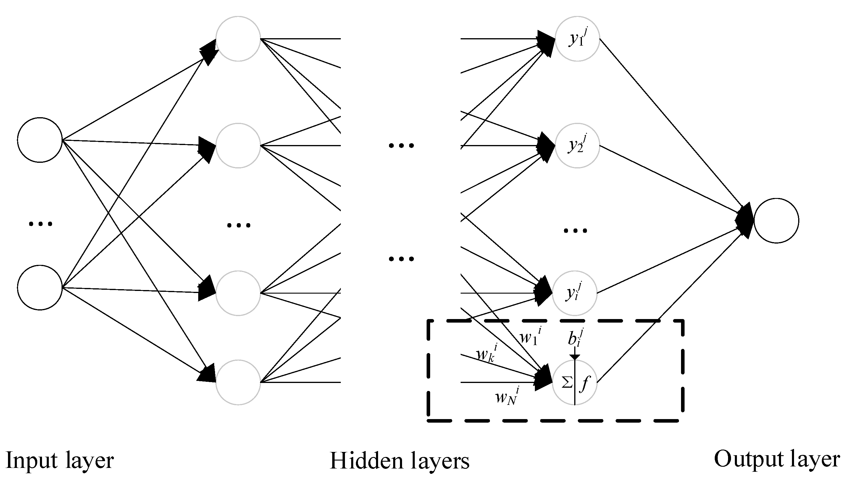
3.3. Neural Network and Training

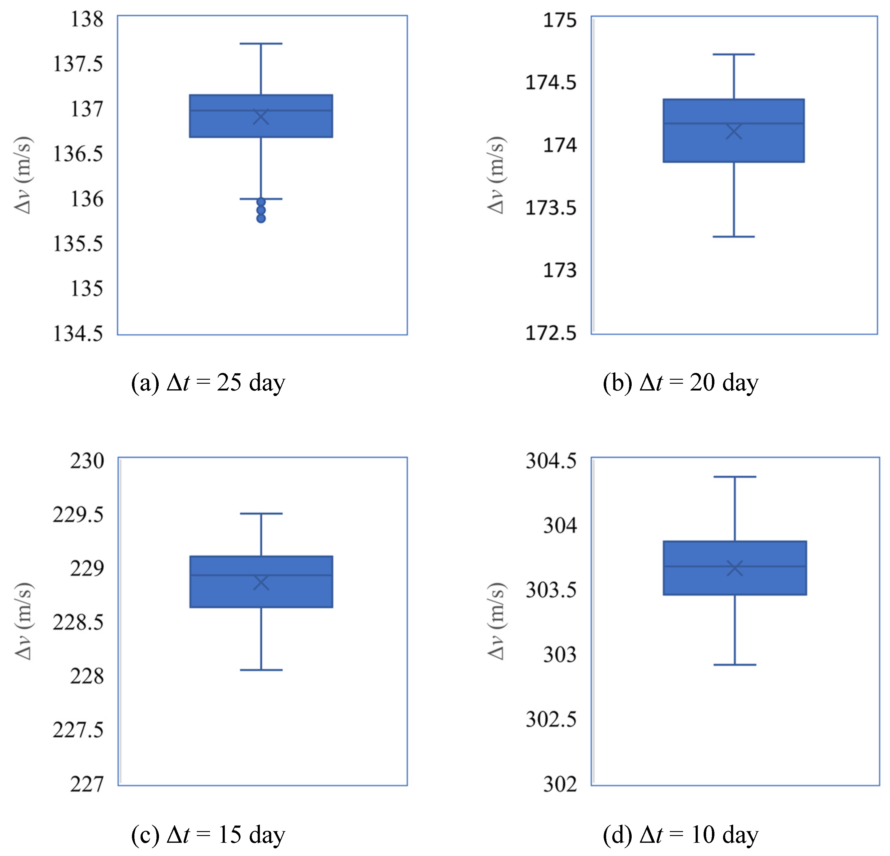
In this study, we applied a multi-layer fully connected neural network [15,16,17] to obtain the surrogate model of the optimal velocity increment. The neural network structure is illustrated in Figure 2.

In Figure 2, the dashed box shows the relationship between the nodes of neighboring layers. The value of the ith node in the jth layer was a weighted sum of the nodes of the previous layer and a constant bias:

$$y_i^j=f({\displaystyle \sum _{k=1}^N{w}_k^i{y}_i^{j-1}+b_i^j})$$

(7)

where N is the number of nodes that are connected to the current node, $w_k^i$ is the weight, $b_i^j$ is the bias, and f is a non-linear function named the activation function. The output was calculated by a given input through multiple layers.

In this study, the input layer was $y^{in}$ and the output layer was the optimal velocity increment. The number of hidden layers was set to 2 and each layer had 60 nodes. A standard rectified linear unit function was set as the activation function. The training process was as follows.

First, a large amount of training data from different inputs was needed. Equation (8) was used to generate the random flight time and the initial and target orbits.

$$\begin{array}{l}{a}_0=\overline{a}+k_1\Delta a_{\max }\\ i_0=\overline{i}+k_2\Delta i_{\max }\\ e_{x0}=k_3{e}_{\max }\cos (k_4\pi )\\ e_{y0}=k_3{e}_{\max }\sin (k_4\pi )\\ {\mathsf{\Omega }}_0=k_5\pi \\ u_0=k_6\pi \\ a_f=\overline{a}+k_7\Delta a_{\max }\\ i_f=\overline{i}+k_8\Delta i_{\max }\\ e_{xf}=k_9{e}_{\max }\cos (k_{10}\pi )\\ e_{yf}=k_9{e}_{\max }\sin (k_{10}\pi )\\ {\mathsf{\Omega }}_f={\mathsf{\Omega }}_0+k_{11}\Delta {\mathsf{\Omega }}_{\max }\\ u_f=k_{12}\pi \\ \Delta t=\Delta t_{\min }+k_{13}\Delta t_{\max }\end{array}$$

(8)

where $k_i,i=1,\mathrm{2...12}$ are random real numbers within [−1, 1] and $k_{13}$ is within (0, 1]. $\Delta {\mathsf{\Omega }}_{\max }$ is the upper limit of the RAAN difference. The optimization method in [9] was applied to obtain the corresponding Δv. Each group of $y^{in}$ and Δv was recorded in the dataset.

The dataset was divided into training (90%) and validating data (10%). Keras, a well-known neural network framework [19], was adopted to complete the training process. For details on the training algorithm, refer to [19]. In this paper, we did not need to adjust the hyperparameters of the neural network by the validating result. Therefore, the functions of the testing data and validating data were almost the same; the validating data could, therefore, prove the precision of the trained neural network.

The training process and the application of the trained neural network are illustrated in Figure 3. To obtain the neural network model, a dataset of optimal velocity increments with different input orbits was generated first. We then obtained the optimal input vector of such a perturbed orbit rendezvous problem and constructed the neural network. The dataset was then used to train the neural network and obtain the weights. Finally, the weights and bias in the neural network were obtained and used in Equation (7) to predict the optimal velocity increment with various input values.

4. Experiments

To validate the proposed neural network design, the problem of the ninth Global Trajectory Optimization Competition (GTOC9) [20] was tested, which provided 123 pieces of debris in LEO that must be removed by multiple orbit transfer vehicles (OTVs) within a given duration. The objective function was to minimize the total launch mass of all that OTVs. It is a complex global optimization problem that has attracted many participants even after the competition. Thus, in the simulation, we trained the neural network to help evaluate the optimal velocity increment of the transfers between the different debris.

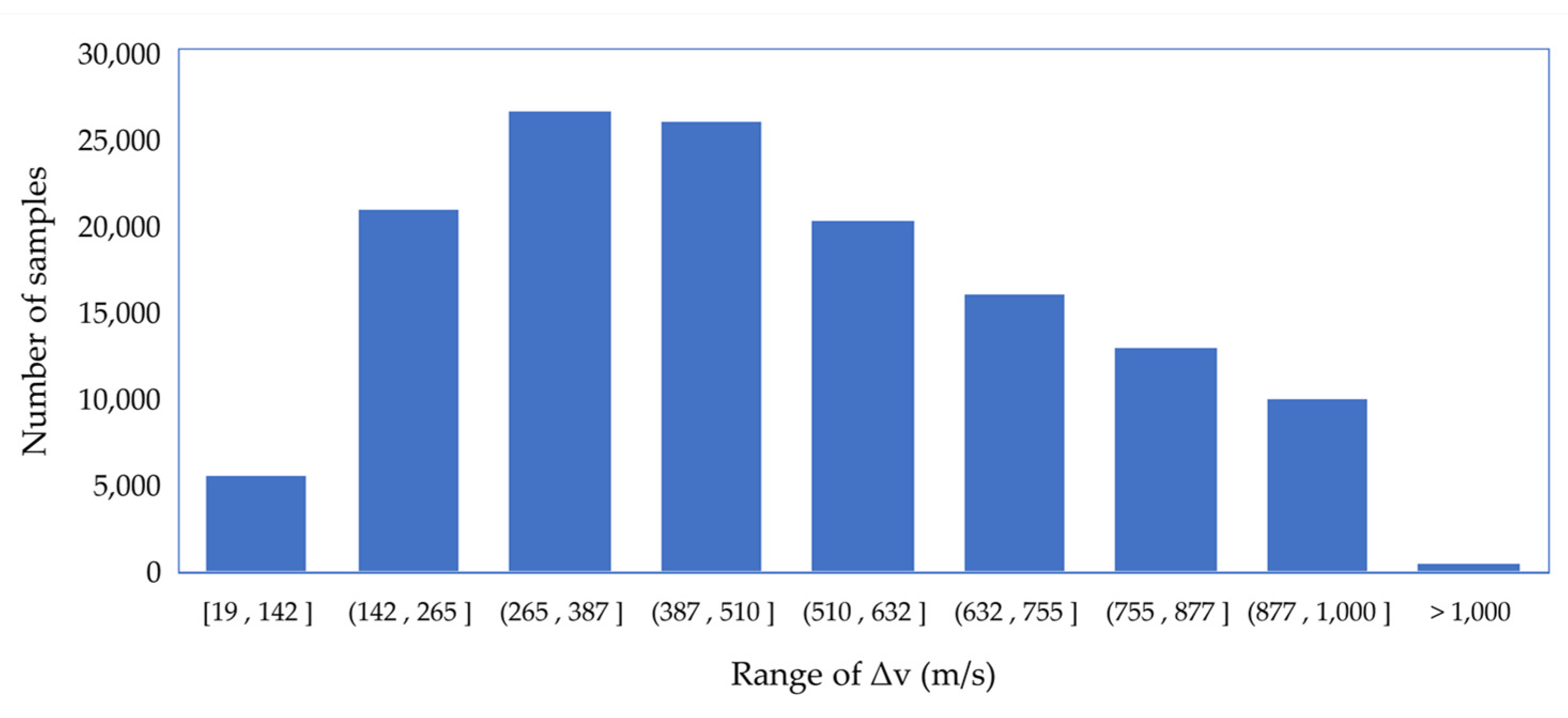
4.1. Dataset Generalization and Training Result

In GTOC9, the orbits of the debris are near-circular, the semi-major axis is centralized at 7100 km, and the inclinations are centralized at 98°. According to Equation (8), we set $\overline{a}$ = 7100 km, $\overline{i}$ = 98°, $\Delta a_{\max }$ = 200 km, $\Delta i_{\max }$ = 2°, $\Delta {\mathsf{\Omega }}_{\max }$ = 10°, and $\Delta t_{\max }$ = 30 d. A dataset consisting of 130,000 groups of input orbits and flight times was generated and the optimal Δv was calculated and recorded. The distribution of Δv is illustrated in Figure 4.

In the Keras framework, the training algorithm was set to “rmsprop” (root mean square propagation), the loss function was “mse” (mean square error), and the batch size was 32. A total of five cases with different numbers of hidden layers and nodes were tested; the results are detailed in

Table 1. Comparison of different neural network parameters.

Number of Hidden Layers	Number of Nodes in Each Hidden Layer	MRE (%)	MAE (m/s)	Time of Each Training Epoch (s)	Training Time (s)	Time of Δv Evaluation (s)
2	30	1.34	5.3	4.6	1380	1.2 × 10−6
2	60	0.96	3.8	5.0	1500	4.8 × 10−6
2	90	0.89	3.7	5.2	1560	1.1 × 10−5
3	60	0.81	3.3	6.0	1800	8.9 × 10−6
4	60	0.79	3.2	7.0	2100	1.3 × 10−5

. The results indicated that 2 hidden layers of 60 nodes were enough to obtain high precision. The mean relative error (MRE) was less than 1% and the mean absolute error (MAE) was less than 4 m/s from the validation data, which was an improvement of more than 50% compared with the results achieved in [17]. This was because the feature vector was extracted more reasonably; the training data were also more precise.

The velocity increments of all transfers using the same input orbits and durations of the solution in [20] (from the Jet Propulsion Laboratory, which won GTOC9) were recalculated by the neural network model presented in this paper. Compared with the results from the Jet Propulsion Laboratory [20], the MRE was less than 4% and close to the semi-analytical method [8].

The correlation between the Δv predicted by the neural network and the optimized Δv in [21] is illustrated in Figure 5, which indicated that the results of two methods were close and the correlation was close to the function y = x. Moreover, the calculation time was only 4.8 × 10⁻⁶ s using an AMD 4.2 GHz CPU, which demonstrated a higher efficiency than previous approximation methods [8,9,10,11].

4.2. Application in Global Optimization

The performance of the proposed neural network was evaluated in the global optimization of a multi-target rendezvous sequence in the GTOC9 problem. Based on the problem description, OTVs can be launched one by one to complete the debris removal mission. Each OTV starts from one debris point and then rendezvous with several targets sequentially. As the optimal velocity required for an orbit rendezvous between two debris objects changes with the orbit elements and transfer time, it is difficult to find the global optimal path of all targets. In the problem description, the maximum duration of the flight time is 25 d between every two debris points; another 5 d is required for the OTV to release a de-orbit package ($\Delta m_{kit}$ = 30 kg) after a rendezvous with target debris. The specific impulse is $I_{sp}$ = 1000 s and the dry mass of the OTV is 2000 kg. Optimizing one OTV is a sub-problem of GTOC9, which aims to find the best path and rendezvous times of given targets to minimize the objective function (the total cost of the OTV mission per unit: million Euro, also MEUR), defined as:

$$J=2\times {10}^{-6}{(m_0-2000)}^2+55$$

(9)

where $m_0$ is the launch mass and can be calculated by the velocity increments of all transfers:

$$\begin{array}{l}{m}_{i-1}=m_i{e}^{\Delta v_i/(I_{sp}g)}+\Delta m_{kit}\\ m_N=2000\mathrm{kg}\end{array}$$

(10)

where g is the gravity acceleration at the sea level, $N$ is the number of debris objects in sequence, $m_i$ represents the mass after the ith transfer, and $\Delta v_i^{}$ is the velocity increment of the ith transfer. The problem is illustrated in Figure 6.

The optimization method in [21] was adopted and the neural network was employed to replace the evaluation of $\Delta v_i$ corresponding with orbit rendezvous between different targets with different transfer times. In the optimization model, the dimension of the decision variables was 2N. The integer variables $\left\{x_{{}_i}\right\},i=1,2\dots N$ represented the order of the rendezvous and the real number variables $\{\Delta t_i^{}\},i=1,2\dots N$ represented the flight times between two debris points. Thus, the start time $t_i^{start}$ and arrival time $t_i^{\mathrm{arrivel}}$ of the ith transfer could be calculated as Equation (11) and the orbit elements of the corresponding targets could be obtained.

$$\begin{array}{l}{t}_i^{start}=\{\begin{array}{l}{t}_{i-1}^{arrivel}+\Delta t_{kit},i>1\\ t_0,i=1\end{array}\\ t_i^{arrivel}=t_i^{start}+\Delta t_i\end{array}$$

(11)

where $t_0$ is the given initial time of the OTV mission and $\Delta t_{kit}$ = 5 d is the time required to release the de-orbit package. Equation (6) was then sequentially applied to calculate the input feature vector. The approximate $\Delta v_i$ could then be obtained by the trained neural network. After all the velocity increments were known, the objective function could be calculated by Equation (9).

The differential evolutionary algorithm was then used to solve this model and obtain the optimal order of the debris and optimal rendezvous times. The results to rendezvous with the same debris objects achieved by the different approximation methods of $\Delta v_i$ are listed in

Table 2. Comparison of different methods.

Model of Velocity Increment	Optimal Order of Debris	Total Δv (m/s)	J (MEUR)	Computational Time (s)
Method in [20]	72, 107, 61, 10, 28, 3, 64, 66, 31, 90, 73, 87, 57, 35, 69, 65, 8, 43, 71, 4, 29	3409.5	97.1	>3600
Method in [21]	72, 107, 61, 73, 3, 69, 64, 66, 31, 10, 90, 87, 57, 35, 28, 65, 8, 43, 71, 4, 29	3357.0	95.6	600
Neural network model in this paper	72, 61, 107, 73, 3, 69, 64, 66, 31, 10, 90, 87, 57, 35, 28, 65, 8, 43, 71, 4, 29	3407.5	97.1	120

, which indicates that the optimal J achieved by the neural network was comparable with other results, but required less calculation using the same AMD 4.2 GHz CPU. Moreover, the test was single-threaded and could be further accelerated because a neural network is easy to parallelize.

5. Conclusions

In this study, we proposed a novel neural network surrogate model for orbit rendezvous between near-circular orbits in low Earth orbits. Most previous methods focused on analytical approximation forms, which require an optimization process and thus lead to an efficiency bottleneck. A few of the latest studies have employed neural networks, but the structures have a lack of theoretical references. In this study, we designed an input layer based on orbit dynamics and normalization was applied to improve the performance. Based on an efficient data generalization process, the network was constructed using a normal training process. The simulation results demonstrated the precision and efficiency of the neural network model. The relative error was less than 1% and was better than that achieved by a similar work [17] based on neural networks. Moreover, the calculation time was 5.8 × 10⁻⁶ s using an ordinary desktop processor and could be directly applied to the global optimization of multi-target rendezvous missions.

References

1. Li, S.; Huang, X.; Yang, B. Review of Optimization Methodologies in Global and China Trajectory Optimization Competitions. Prog. Aerosp. Sci. 2018, 102, 60–75. [Google Scholar] [CrossRef]
2. Vallado, D.A. Fundamentals of Astrodynamics and Applications, 2nd ed.; Microscosm Press: Torrance, CA, USA, 2001; pp. 757–800. [Google Scholar]
3. Casalino, L.; Dario, P. Active Debris Removal Missions with Multiple Targets. In Proceedings of the AIAA/AAS Astrodynamics Specialist Conference, San Diego, CA, USA, 4–7 August 2014. [Google Scholar]
4. Yang, Z.; Luo, Y.Z.; Zhang, J. Two-Level Optimization Approach for Mars Orbital Long-Duration, Large Non-Coplanar Rendezvous Phasing Maneuvers. Adv. Space Res. 2013, 52, 883–894. [Google Scholar] [CrossRef]
5. Zhang, T.J.; Shen, H.; Yang, Y. Ant Colony Optimization-Based Design of Multiple-Target Active Debris Removal Mission. Trans. Jpn. Soc. Aeronaut. Space Sci. 2018, 61, 201. [Google Scholar] [CrossRef] [Green Version]
6. Barea, A.; Urrutxua, H.; Cadarso, L. Large-Scale Object Selection and Trajectory Planning for Multi-Target Space Debris Removal Missions. Acta Astronaut. 2020, 170, 289–301. [Google Scholar] [CrossRef]
7. Cerf, M. Multiple Space Debris Collecting Mission: Optimal Mission Planning. J. Optim. Theory Appl. 2015, 167, 195–218. [Google Scholar] [CrossRef] [Green Version]
8. Huang, A.Y.; Luo, Y.Z.; Li, H.N. Fast Estimation of Perturbed Impulsive Rendezvous via Semi-Analytical Equality-Constrained Optimization. J. Guid. Control Dyn. 2020, 43, 2383–2390. [Google Scholar] [CrossRef]
9. Huang, A.Y.; Luo, Y.Z.; Li, H.N. Fast Optimization of Impulsive Perturbed Orbit Rendezvous Using Simplified Parametric Model. Astrodynamics 2021, 5, 391–402. [Google Scholar] [CrossRef]
10. Chen, S.Y.; Baoyin, H.X. Analytical Estimation of the Velocity Increment in J2-Perturbed Impulsive Transfers. J. Guid. Control Dyn. 2022, 45, 310–319. [Google Scholar] [CrossRef]
11. Shen, H.X.; Casalino, L. Simple ΔV Approximation for Optimization of Debris-to-Debris Transfers. J. Spacecr. Rocket. 2021, 58, 575–580. [Google Scholar] [CrossRef]
12. Schmidhuber, J. Deep learning in neural networks: An overview. Neural Netw. 2015, 61, 85–117. [Google Scholar] [CrossRef] [Green Version]
13. Izzo, D.; Märtens, M.; Pan, X. A survey on artificial intelligence trends in spacecraft guidance dynamics and control. Astrodynamics 2019, 4, 287–299. [Google Scholar] [CrossRef]
14. Diao, Y.; Pu, J.; Xu, H.; Mu, R. Orbit-Injection Strategy and Trajectory-Planning Method of the Launch Vehicle under Power Failure Conditions. Aerospace 2022, 9, 199. [Google Scholar] [CrossRef]
15. Li, H.; Chen, S.; Izzo, D. Deep networks as approximators of optimal low-thrust and multi-impulse cost in multitarget missions. Acta Astronaut. 2020, 166, 469–481. [Google Scholar] [CrossRef]
16. Zhu, Y.H.; Luo, Y.Z. Fast Evaluation of Low-Thrust Transfers via Multilayer Perceptions. J. Guid. Control Dyn. 2019, 42, 2627–2637. [Google Scholar] [CrossRef]
17. Zhu, Y.H.; Luo, Y.Z. Fast Approximation of Optimal Perturbed Long-Duration Impulsive Transfers via Artificial Neural Networks. IEEE Trans. Aerosp. Electron. Syst. 2021, 57, 123–1138. [Google Scholar] [CrossRef]
18. More, J.J.; Garbow, B.S.; Hillstrom, K.E. User Guide for MinPack-1; Report No. ANL-80-74; Argonne National Lab.: Lemont, IL, USA, 1980. [Google Scholar]
19. Izzo, D.; Martens, M. The Kessler Run: On the Design of the GTOC9 Challenge. Acta Futura 2018, 11, 11–24. [Google Scholar]
20. Petropoulos, A.; Grebow, D.; Jones, D. GTOC9: Methods and Results from the Jet Propulsion Laboratory Team. Acta Futura 2018, 11, 25–35. [Google Scholar]
21. Huang, A.Y.; Luo, Y.Z.; Li, H.N. Global Optimization of Multiple-Spacecraft Debris Removal Mission via Problem Decomposition and Dynamics-Guide Evolution Approach. J. Guid. Control Dyn. 2022, 45, 171–178. [Google Scholar] [CrossRef]
Figure 1. Box diagram of optimized velocity increments with different orbits and the same x.
Mathematics 10 02489 g001
Figure 2. Structure of the multi-layer neural network.
Mathematics 10 02489 g002
Figure 3. Flowchart of the training and application of the neural network.
Mathematics 10 02489 g003
Figure 4. Distribution of sampling Δv at different ranges.
Mathematics 10 02489 g004
Figure 5. Correlation between the proposed neural network and approximate method in Petropoulos 2018.
Mathematics 10 02489 g005
Figure 6. Optimization of a sequence (N = 5).
Mathematics 10 02489 g006