A Model for the Proliferation–Quiescence Transition in Human Cells

Abstract

The process of revitalising quiescent cells in order for them to proliferate plays a pivotal role in the repair of worn-out tissues as well as for tissue homeostasis. This process is also crucial in the growth, development and well-being of higher multi-cellular organisms such as mammals. Deregulation of proliferation-quiescence transition is related to many diseases, such as cancer. Recent studies have revealed that this proliferation–quiescence process is regulated tightly by the $Rb-E2F$ bistable switch mechanism. Based on experimental observations, in this study, we formulate a mathematical model to examine the effect of the growth factor concentration on the proliferation–quiescence transition in human cells. Working with a non-dimensionalised model, we prove the positivity, boundedness and uniqueness of solutions. To understand model solution behaviour close to bifurcation points, we carry out bifurcation analysis, which is further illustrated by the use of numerical bifurcation analysis, sensitivity analysis and numerical simulations. Indeed, bifurcation and numerical analysis of the model predicted a transition between bistable and stable states, which are dependent on the growth factor concentration parameter ($GF$). The derived predictions confirm experimental observations.

1. Introduction

The human body consists of approximately ${10}^{13}$–${10}^{14}$ cells. A large proportion of these cells are quiescent, a biochemically distinct state of growth arrest from which cells can re-enter the cell cycle [1]. The proportion of quiescent cells consists of cells that can no longer be re-activated to re-enter the cell cycle, and cells that can be re-activated to re-enter the cell cycle in response to growth factor signals under normal physiological conditions [2]. The cell cycle comprises four phases, namely: $G_1$ (first gap phase), S (synthesis phase), $G_2$ (second gap phase) and M (mitosis), where gap phases refer to the time interval between the synthesis phase and mitosis [3,4]. Here, mitosis refers to the process by which a single cell divides into two identical daughter cells. The commitment of a cell to cell division is driven by growth factor signals. The availability of sufficient growth factors just beyond a certain point between $G_1$ and S, known as the restriction point, leads to the progression of the cell cycle process, otherwise the cell enters a reversible state of growth arrest $\left(G_0\right)$ [5,6,7,8,9,10,11,12].

Mammalian cellular homeostasis (the state of steady internal, physical, and chemical conditions maintained by cells) depends on the ability of cells to reversibly switch between quiescence and proliferation [13]. This mechanism is crucial for tissue repair and regeneration and is fundamental to the growth, development and well-being of mammals. The decision by cells to exit or enter quiescence is dysregulated in cancer and degenerative diseases [14,15,16]. Therefore, understanding the molecular mechanisms that control the reversible transition between quiescence and proliferation is crucial and remains a challenging problem in biological and medical sciences. In the 1970s and 1980s, three classes of models were proposed to describe the transition between cellular quiescence and proliferation [17]. These include: the “transition probability” models [18,19,20,21], the “growth controlled” models [22,23] and the hybrid models [24,25]. Hybrid models were developed by integrating transition probability- and growth-controlled models [24,25]. Though these models are coherent with diverse experimental data, they lack depth, since they are descriptive. Modelling proliferation–quiescence transition has shifted from this approach since the discovery, in the contexts of molecular and cell biology, of certain genes that regulate proliferation–quiescence transition [17]. Continuum mathematical models describing the temporal dynamics to provide insights into proliferation–quiescence transition within the cell cycle using gene regulatory networks have been proposed in the last two decades [26,27,28,29,30,31,32,33,34,35]. Limit cycles [28,30,32], cell-mass-regulated bi-stable systems [25,34,36], bi-stable and excitable systems [33,37] and transient processes [26,29,38] are examples of the cell-cycle dynamics deduced through cell-cycle modelling. It has been demonstrated experimentally that proliferation–quiescence transition is controlled by the $Rb-E2F$ signalling network, which acts as a bi-stable switch [17]. Here, $Rb$ and $E2F$ represent the Retinoblastoma and Transcription factors respectively. Previously, models for the regulation of the $Rb-E2F$ have been put forward and simulated [29,32,38], with more details provided in the model proposed by Aguda and Tang [38]. At the heart of the regulation of the $Rb-E2F$ signalling network are: cyclin $D\left(CycD\right),$ cyclin $E\left(CycE\right),$ cyclin $A\left(CycA\right),$ cyclin-dependent kinases $\left(CDKs\right),$ family of transcription factors $E2F,Myc$ and the retinoblastoma $\left(Rb\right)$ family of proteins [39,40]. The retinoblastoma $\left(Rb\right)$ protein family is responsible for regulating proliferation in most cells. The $E2F$ family of transcription factors is responsible for the regulation of genes involved in $DNA$ replication and cell cycle progression [41,42]. Interactions among these regulators have been outlined and verified experimentally [17]. However, due to the complex nature of the $Rb-E2F$ network, which consists of criss-crossing linkages, a clear description of the proliferation–quiescence transition is elusive. In this study, we simplify the $Rb-E2F$ signalling network that has been theoretically and experimentally verified in [43,44,45,46], and formulate an activator-inhibitor model system following the same philosophy as that proposed by Tyson et al. in [25], to analyse the proliferation–quiescence transition. To investigate the dynamics of the $Rb-E2F$ signalling network describing proliferation–quiescence transition, we have taken the approach of combining redundant and overlapping cellular activities and collapsing linear cascades, as presented by Yao et al. [42], to simplify the model to three nodes connected by activation and inhibition links, as experimentally verified in [45]. Although the terms activation and inhibition are generally used in the literature, in this study we will also refer to these molecular processes as the production/synthesis and degradation/removal of abundant species, respectively. In addition, we consider the conservation of the total concentration of the $Rb$ family of proteins and show through bifurcation and numerical analysis that the resulting system generates a set of three dynamical behaviours shown in experiments [1,2,17]; namely, stability, bistability and stability when the growth factor concentration ($GF$) is varied. Bifurcation and numerical analysis also show that quiescence is achieved under low growth factor stimulation and proliferation requires strong growth-factor stimulation.

This paper is organised as follows: in Section 2, we utilise the current understanding of activator-inhibitor systems and apply biologically reasonable assumptions to motivate a system of non-linear ordinary differential equations (ODEs) and describe the pertinent interactions. In the same section, we non-dimensionalise the system, outline positivity, boundedness and prove the existence and uniqueness of solutions. This section ends with a further study of the non-linear ODE system to gain insights into its stability behaviour. In Section 3, we conduct a bifurcation analysis of the model to analyse the effect of varying the growth factor concentration on the steady states of the system. We also conduct numerical simulations to illustrate, computationally, the theoretical results. The last part of Section 3 presents sensitivity analysis for parameters of the system. We discuss the interpretations and implications of our results in Section 4. Finally, in Section 5, we discuss the limitations of our study and present possible future research problems.

2. Materials and Methods

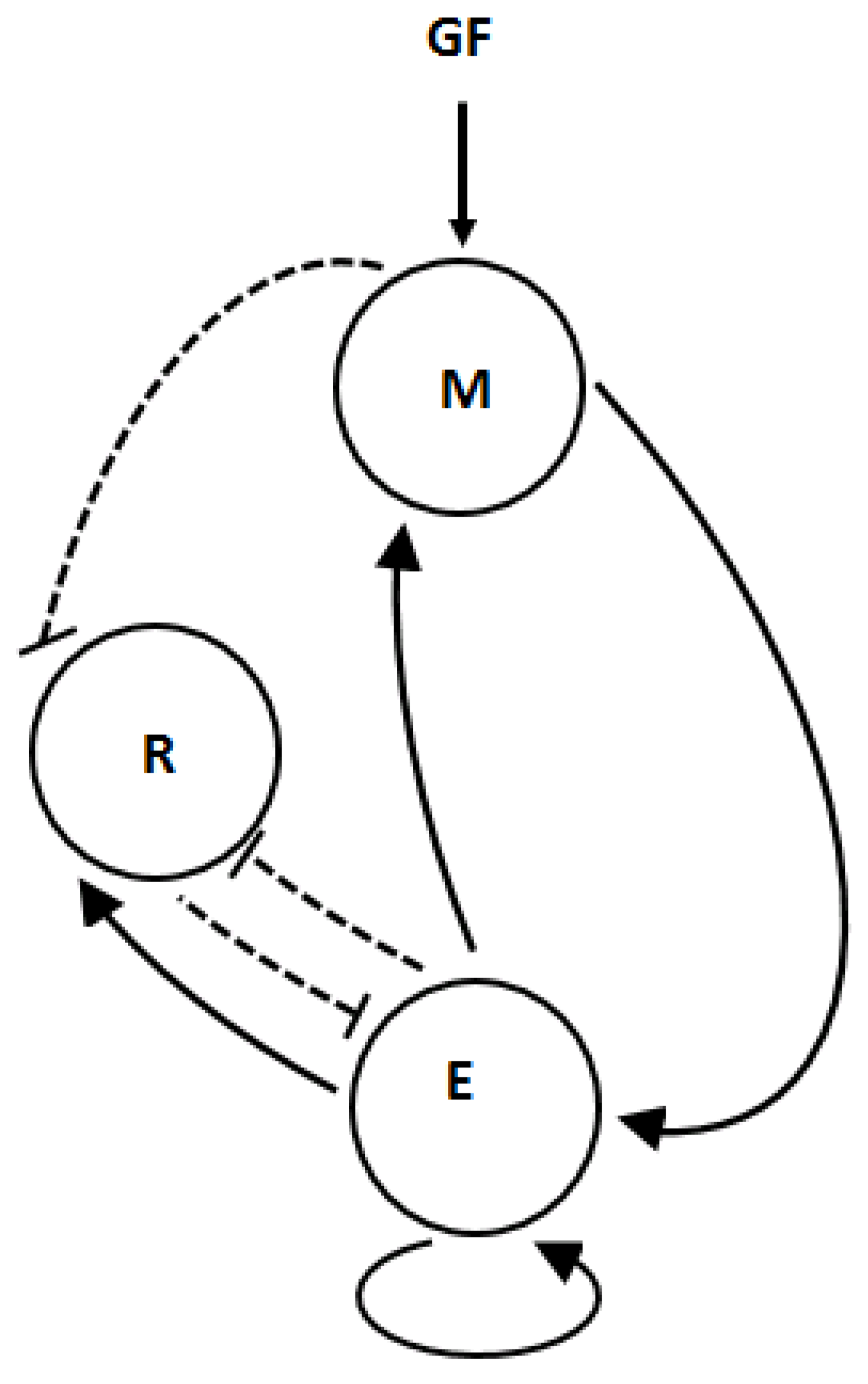
2.1. Proliferation–Quiescence Dynamics Model

Our mathematical model is formulated based on first principles by first simplifying the $Rb-E2F$ model studied by Yao et al. [17], collapsing all the several reaction networks into three main nodes denoted by: R, M and E and thus reducing the reaction links from 10 to 8, as shown in Figure 1. The R node consists of the $Rb$ family of proteins $(Rbp107 \mathrm{and} Rbp108),$ the E node consists of the family of transcription factors $E2F,$ Cyclin E and Cyclin $A,$ and the M node consists of cyclin D and $Myc$. Experimentally, it is observed that R proteins are conserved throughout, while those of M and E are not [40]. Due to lack of experimental justifications for some reactions, and following other published works [12,40], in formulating our model we will employ Michaelis–Menten kinetics, mass action as well as the Hill function [47]. Michaelis–Menten kinetics describe the rate of enzymatic reactions by relating reaction rates to the concentration of a substrate, while the law of mass action states that the rate of a chemical reaction is directly proportional to the product of the activities or concentrations of the reactants [48,49].

Yao et al. [17] represented the three respective nodes by symbols: $RP$, $EE$ and $MD$. These nodes are connected by 10 regulatory linkages. In their model, they assumed activation of the three species $RP$, $EE$ and $MD$ by Hill functions of the form: $\frac{A^n}{K^n+\left[A^n\right]}$, where A represents any of the three species $RP$, $MD$ or $EE$, K is a Michaelis–Menten constant and $1\le n\le 10$. In addition, they assumed that the inhibition of $RP$, $EE$ and $MD$ was through mass action kinetics. Of interest was their exclusion of the constitutive synthesis of $EE$ together with its self-activation and the conservation of mass of the $RP$ family of proteins, which we will consider in our model. Moreover, they considered self-inhibition of $EE$ and inhibition of $EE$ by $MD$, which we removed in our model. The simplified network self-reorganises to form an activator-inhibitor network, as shown in Figure 1.

In our model formulation, we ignore the spatial localisation of the proteins; such an extension forms part of our current studies and is beyond the scope of this work. We note, however, that such an approach leads naturally to partial differential equations. The resulting model, when spatial effects are neglected, is given in terms of a system of non-linear ordinary differential equations (ODEs) describing the rate of change in the concentrations of $M\left(t\right)$, $R\left(t\right)$ and $E\left(t\right)$. The main novelty of the model is the use of the Hill function with $n=2$ to describe kinetics with saturation. The model is formulated based on the following assumptions:

1

The production of $M\left(t\right)$ is through mass action by extra-cellular growth signals $GF$ and by $E\left(t\right)$, which is modelled using Michaelis–Menten kinetics, whereas its decay is modelled by mass action. Yao et al. [2] considered Michaelis–Menten kinetics for the production of $M\left(t\right)$ through extra-cellular growth signals.

2

The activation of $R\left(t\right)$ is enhanced by $E\left(t\right)$ and its inhibition is intensified by $M\left(t\right)$ and $E\left(t\right)$, which are both modelled using mass action. It is pertinent to note that, in this study, we assume conservation of mass for the $Rb$ family of proteins, which was not considered in [2]. In addition, we assume self-activation and inhibition of $R\left(t\right)$ using the Hill function with $n=2$. On the contrary, Yao et. al. [2] modelled the production and depletion of $R\left(t\right)$ using Michaelis–Menten kinetics and mass action, respectively, and self-activation and de-activation were not considered.

3

$E\left(t\right)$ is synthesised, cf. [40], with the use of Michaelis–Menten kinetics and its synthesis is enhanced by $M\left(t\right)$ with the use of a Hill function with $n=2$, while its decay is enhanced by $R\left(t\right)$ with the use of mass action. On the contrary, the authors in [2] did not consider constitutive synthesis of $E\left(t\right),$ which has been observed experimentally as indicated in [40].

The main novelty of our proposed model is that we consider mass conservation of the $Rb$ family of proteins represented by $R\left(t\right)$ existing in both hypo-phosphorylated form denoted by $R_u\left(t\right)$ and hyper-phosphorylated form denoted by $R_p\left(t\right);$ whereas in [42] it was assumed that the concentration of the $Rb$ family of proteins was abundant and hence there was no mass conservation. This assumption makes our model more realistic, as the transition from cellular quiescence to proliferation is dependent on the cycling between the hyper-phosphorylated and hypo-phosphorylated forms of $Rb$ family of proteins mediated by cyclin-dependent kinases. Hyperphosphorylation of $Rb$ enhances proliferation, whereas hypo-phosphorylated $Rb$ enhances quiescence [50]. In addition, some reaction pathways were not considered in [2], including constitutive synthesis of E and the simple mass action for the activation of $R\left(t\right)$. Therefore, employing mass conservation, the total concentration of $R\left(t\right)$ is such that:

$$R_u\left(t\right)+R_p\left(t\right)=R_T=Constant.$$

The state variable $R\left(t\right)$ denotes the concentration of $R_p\left(t\right)$ at time t in the model. $R_u\left(t\right)$ corresponds to the inactive term $R_T-R$ used in Equation (1c). Therefore, the time evolution of $M\left(t\right)$, $E\left(t\right)$ and $R\left(t\right)$ are, respectively, described by the following system of non-linear ordinary differential equations (ODEs):

$$\begin{array}{cc}\frac{dM}{dt}=\hfill & \underset{production of M by GF}{\underbrace{{\alpha }_{1}GF}}+\underset{production of M by E}{\underbrace{{\displaystyle \frac{{\beta }_{1}ME}{k_1+E}}}}-\underset{decay ofM}{\underbrace{\delta M}},\hfill \end{array}$$

(1a)

$$\begin{array}{cc}\hfill {\displaystyle \frac{dE}{dt}}=& \underset{E baseline value}{\underbrace{{\alpha }_6}}+\underset{E constitutive-synthesis}{\underbrace{{\displaystyle \frac{{\alpha }_{4}E}{{\alpha }_8+E}}}}+\underset{Production of E by M}{\underbrace{{\displaystyle \frac{{\beta }_{4}E{M}^2}{k_{r_3}^2+M^2}}}}-\underset{removal of E by R}{\underbrace{{\alpha }_{5}RE}},\hfill \end{array}$$

(1b)

$$\begin{array}{c}\hfill \begin{array}{cc}\hfill {\displaystyle \frac{dR}{dt}}=& \underset{Activation of R by E}{\underbrace{{\beta }_2(R_T-R)E}}+\underset{R baseline activation}{\underbrace{{\displaystyle \frac{{\beta }_3{(R_T-R)}^2}{k_{r_1}^2+{(R_T-R)}^2}}}}-\underset{Inhibition of R by M}{\underbrace{{\alpha }_{2}RM}}-\underset{inhibition of R by E}{\underbrace{{\alpha }_{3}RE}}\hfill \\ & \hspace{1em}-\underset{R baseline inhibition}{\underbrace{{\displaystyle \frac{{\beta }_5{R}^2}{k_{r_2}^2+R^2}}}}.\hfill \end{array}\end{array}$$

(1c)

The system is closed with non-negative initial conditions $M\left(0\right)=M_0$, $E\left(0\right)=E_0$, and $R\left(0\right)=R_0$, $0\le M\left(t\right),E\left(t\right)$ and $0\le R\left(t\right)\le R_T$. In our model, we consider M and E families of proteins to exist in abundance; hence, there is no conservation of mass, unlike the $Rb$ family of proteins, which is conserved as outlined in the model formulation. This implies, that for some appropriate model parameter values, M and E might be unbounded. Model parameters are chosen based on a previous modelling study on the $Rb-E2F$ pathway [17]. All model parameters are strictly positive and their values, units and physical meaning are described in

Table 1. Parameters used for simulations and bifurcation analysis. Parameter values are taken from [17,42] and some of them adjusted to illustrate the qualitative dynamics. Here, U represents the unit of concentration and s the unit of time t.

Parameter	Description	Value	Units	Reference
${\alpha }_1$	Growth factors activation rate	1	${\mathrm{s}}^{-1}$	[17]
$GF$	Growth factors concentration	varies	U	[42]
$\delta$	Inhibition rate of M	1.001	${\mathrm{s}}^{-1}$	[17]
$k_1$	Michaelis–Menten constant	1	U	[42]
${\beta }_1$	Activation rate of M	1	${\mathrm{s}}^{-1}$	[42]
${\beta }_2$	Activation of R protein family	1	U${}^{-1}{\mathrm{s}}^{-1}$	[42]
${\alpha }_3$	Inhibition rate of R by E	1	U${}^{-1}{\mathrm{s}}^{-1}$	Estimate
${\alpha }_2$	Inhibition rate of R by M	1	U${}^{-1}{\mathrm{s}}^{-1}$	Estimate
${\beta }_3$	R baseline inhibition rate	1	U${\mathrm{s}}^{-1}$	Estimate
$R_T$	Total concentration of R	5	U	[40]
${\alpha }_4$	E self activation rate	0.02	U${\mathrm{s}}^{-1}$	[17]
${\beta }_4$	Activation rate E by M	0.02	${\mathrm{s}}^{-1}$	[17]
${\beta }_5$	R baseline inhibition rate	1	U${\mathrm{s}}^{-1}$	Estimate
${\alpha }_6$	E constitutive activation rate	0.001	${\mathrm{s}}^{-1}$	[40]
${\alpha }_8$	Michaelis–Menten constant	0.92	U	[42]
${\alpha }_5$	Inhibition rate of E by R	0.01	U${}^{-1}{\mathrm{s}}^{-1}$	[42]
$k_{r_1}$	Michaelis–Menten constant	0.05	U	[42]
$k_{r_2}$	Michelis–Menten constant	1	U	[42]
$k_{r_3}$	Michaelis–Menten constant	1	U	[42]

.

2.2. Mathematical Analysis of the Model

In this section, we non-dimensionalise system (1) so that it is unit free for purposes of mathematical analysis, including proving positivity, boundedness, existence and uniqueness of solutions as well as performing the sensitivity analysis. However, numerical bifurcation and numerical simulations were performed on the dimensional model. This is meant to preserve the original concentration of species $GF$, which appears in Equation (1a).

2.3. Non-Dimensionalisation

There are nineteen parameters in system (1). We can reduce the number of parameters to sixteen by defining new coordinates $M=X{x}^{*}$, $E=Y{y}^{*}$, $R=Z{z}^{*}$ and $t=T\tau$, where X, Y, Z and t are constant (dimension carrying) scales, to be chosen and $x^{*}$; $y^{*}$; $z^{*}$; $\tau$ are the numerical (dimensionless) variables. Substituting these into (1) and letting $a_1=\frac{{\alpha }_{1}GF}{{\alpha }_4}$, $a_2=\frac{{\beta }_1{\alpha }_8}{{\alpha }_4}$, $a_3=\frac{k_1}{{\alpha }_8}$, $a_4=\frac{\delta {\alpha }_8}{{\alpha }_4}$, $a_5=\frac{{\beta }_2{\alpha }_8^2}{{\alpha }_4}$, $a_6=\frac{R_T}{{\alpha }_8}$, $a_7=\frac{{\beta }_3}{{\alpha }_4}$, $a_8=\frac{k_{r_1}^2}{{\alpha }_8^2}$, $a_9=\frac{{\alpha }_2{\alpha }_8^2}{{\alpha }_4}$, $a_{10}=\frac{{\alpha }_3{\alpha }_8^2}{{\alpha }_4}$, $a_{11}=\frac{{\beta }_5}{{\alpha }_4}$, $a_{12}=\frac{k_{r_2}^2}{{\alpha }_8^2}$, $a_{13}=\frac{{\beta }_4{\alpha }_8}{{\alpha }_4}$, $a_{14}={\displaystyle \frac{k_{r_3}^2}{{\alpha }_8^2}}$, $a_{15}=\frac{{\alpha }_6{\alpha }_8}{{\alpha }_4}$ and $a_{16}=\frac{{\alpha }_5{\alpha }_8^2}{{\alpha }_4}$, and, dropping * so that $x^{*}=x$, $y^{*}=y$ and $z^{*}=z$, we obtain the non-dimensional system:

$$\begin{array}{cc}\hfill \frac{dx}{dt}=& a_1+\frac{a_{2}xy}{a_3+y}-a_{4}x,\hfill \end{array}$$

(2a)

$$\begin{array}{cc}\hfill \frac{dy}{dt}=& a_{16}+\frac{y}{1+y}+\frac{a_{13}{x}^{2}y}{a_{14}+x^2}-a_{15}yz,\hfill \end{array}$$

(2b)

$$\begin{array}{cc}\hfill \frac{dz}{dt}=& a_5(a_6-z)y+\frac{a_7{(a_6-z)}^2}{a_8+{(a_6-z)}^2}-a_{9}xz-a_{10}yz-\frac{a_{11}{z}^2}{a_{12}+z^2},\hfill \end{array}$$

(2c)

with positive initial conditions $x\left(0\right)=x_0, y\left(0\right)=y_0 and z\left(0\right)=z_0$ and positive constant parameters $a_1,\cdots ,a_{16}.$

2.4. Positivity, Boundedness and Existence and Uniqueness of Solutions

We first show thatsystem (2), associated with initial conditions, has a unique local solution.

Lemma 1

(Local existence and uniqueness). System (2), associated with the initial condition$\left(x\right(0),y(0),andz(0\left)\right)$, has a unique local solution in the interval $(0,T)$ for some $T>0.$

Proof. 

System (2) can be written in matrix form, as follows:

$$\frac{d\overrightarrow{x}}{dt}=\left[\begin{array}{c}\frac{dx}{dt}\\ \frac{dy}{dt}\\ \frac{dz}{dt}\end{array}\right]=\overrightarrow{f}\left(\overrightarrow{x}\right)=\left[\begin{array}{c}{f}_1(x,y,z)\\ f_2(x,y,z)\\ f_3(x,y,z)\end{array}\right],$$

(3)

for $\overrightarrow{x}=\overrightarrow{x}\left(t\right)={\left(x\left(t\right),y\left(t\right),z\left(t\right)\right)}^T$ and

$$\begin{array}{ccc}& & f_1(x,y,z):=a_1+\frac{a_{2}xy}{a_3+y}-a_{4}x,\hfill \\ & & f_2(x,y,z):=a_{16}+\frac{y}{1+y}+\frac{a_{13}{x}^{2}y}{a_{14}+x^2}-a_{15}yz,\hfill \\ & & f_3(x,y,z):=a_5(a_6-z)y+\frac{a_7{(a_6-z)}^2}{a_8+{(a_6-z)}^2}-a_{9}xz-a_{10}yz-\frac{a_{11}{z}^2}{a_{12}+z^2}.\hfill \end{array}$$

It follows that $\overrightarrow{f}$ is Lipschitz continuous, i.e., there exists a constant $L\ge 0$ such that $\Vert \overrightarrow{f}\left({\overrightarrow{x}}_1\right)-\overrightarrow{f}\left({\overrightarrow{x}}_2\right)\Vert \le L\Vert {\overrightarrow{x}}_1-{\overrightarrow{x}}_2\Vert$, for all ${\overrightarrow{x}}_1$, ${\overrightarrow{x}}_2\in D,$ for any bounded region D in ${\mathbb{R}}_{+}^3.$ Then, local existence and uniqueness of solutions is established by the classic theory, cf. [51]. □

Next, the positivity of solutions of (2) is established; hence, the feasibility of solutions for the study of the underlying biological problem is guaranteed.

Lemma 2

(Positivity). If the initial condition in system (2) satisfies $x\left(0\right)>0$, $y\left(0\right)>0$, $z\left(0\right)>0$, then the solution $\left(x\right(t), y(t), z(t\left)\right)$ of (2) will remain in ${\mathbb{R}}_{+}^3$ for all $t\in [0,T]$, where $T>0$ stands for the maximum existence time guaranteed by Lemma 1.

Proof. 

We must prove that $\left(x\right(t),y(t),z(t\left)\right)$ will remain in ${\mathbb{R}}_{+}^3$ for any $t\in (0,T),$ where $T>0$ is the maximum existence time. Since $x\left(0\right)>0$, $y\left(0\right)>0$, $z\left(0\right)>0$ then, by a continuity argument, there exists $t_1>0$ such that $(x\left(t\right),y\left(t\right),z\left(t\right))\in {\mathbb{R}}_{+}^3$ for all $t\in [0,t_1].$ Thus, recalling that all parameters used in system (2) are positive, we derive the following inequalities in the interval $(0,t_1)$

$$\begin{array}{cc}\hfill \frac{dx}{dt}=& a_1+\frac{a_{2}xy}{a_3+y}-a_{4}x\ge -a_{4}x,\hfill \end{array}$$

(4a)

$$\begin{array}{cc}\hfill \frac{dy}{dt}=& a_{16}+\frac{y}{1+y}+\frac{a_{13}{x}^{2}y}{a_{14}+x^2}-a_{15}yz\ge -a_{15}yz,\hfill \end{array}$$

(4b)

$$\begin{array}{cc}\hfill \frac{dz}{dt}=& a_5(a_6-z)y+\frac{a_7{(a_6-z)}^2}{a_8+{(a_6-z)}^2}-a_{9}xz-a_{10}yz-\frac{a_{11}{z}^2}{a_{12}+z^2}\ge -a_{5}z-a_{9}xz-a_{10}yz.\hfill \end{array}$$

(4c)

Now, integrating the above differential equation inequalities in the interval $[t_1,T)$, we obtain

$$\begin{array}{ccc}& & x\left(t\right)\ge A_0{e}^{-a_4(t-t_1)}>0,\hfill \\ & & y\left(t\right)\ge C_0{e}^{-a_{15}{\int }_{t_1}^{t}z\left(t\right)dt}>0,\hfill \\ & & z\left(t\right)\ge B_0{e}^{-a_9{\int }_{t_1}^{t}x\left(t\right)dt-(a_5+a_{10}){\int }_{t_1}^{t}y\left(t\right)dt}>0,\hfill \end{array}$$

for some positive constants $A_0,B_0,C_0.$ Thus, for all $t\in [0,t_1], x\left(t\right), y\left(t\right),and z\left(t\right)$ will remain in ${\mathbb{R}}_{+}^3$. Repeating this argument, we can prove that $(x\left(t\right),y\left(t\right),z\left(t\right))\in {\mathbb{R}}_{+}^3$ for any $t\in (0,T)$, and this completes the proof. □

Lemma 3

(Boundedness). There exists $x_v, y_v, z_v>0$ such that ${lim\; sup}_{t\to T}x\left(t\right)\le x_v$, ${lim\; sup}_{t\to T}y\left(t\right)\le y_v$ and ${lim\; sup}_{t\to T}z\left(t\right)\le z_v$ provided that $min(\theta ,\varphi )>0$ where $\theta :=a_4-a_2$ and $\varphi :=a_{15}{z}_v-a_{13}$. Here, T is the maximum existence time for system (2) given by Lemma 1.

Proof. 

Since all involved constants $a_i,i=1,\cdots ,16$ are positive, thanks to Lemma 2 we can deduce that

$$\begin{array}{c}\hfill \underset{z\to a_6}{lim}{\displaystyle \frac{dz}{dt}}=-a_6{a}_{9}x-a_6{a}_{10}y-{\displaystyle \frac{a_{11}{a}_6^2}{a_{12}+a_6^2}}\le 0,\end{array}$$

which implies that there exists $z_v>0$ such that ${lim\; sup}_{t\to T}z\left(t\right)\le z_v;$ hence, $z\left(t\right)$ is bounded in $[0,T].$ By making the substitution $z=z_v$ we also obtain that

$$\begin{array}{cc}\hfill {\displaystyle \frac{dx}{dt}}+{\displaystyle \frac{dy}{dt}}=& a_1+\frac{a_{2}xy}{a_3+y}-a_{4}x+a_{16}+\frac{y}{y+1}+\frac{a_{13}{x}^{2}y}{a_{14}+x^2}-a_{15}y{z}_v.\hfill \\ \hfill & \le a_1+a_{2}x-a_{4}x+a_{16}+1+a_{13}y-a_{15}y{z}_v,\hfill \\ \hfill & \le a_1+a_{16}+1-x(a_4-a_2)-y(a_{15}{z}_v-a_{13}).\hfill \end{array}$$

Setting $\theta :=a_4-a_2$ and $\varphi :=a_{15}{z}_v-a_{13},$ provided that $min(\theta ,\varphi )>0$, then it follows that

$$\begin{array}{ccc}\hfill {\displaystyle \frac{d(x+y)}{dt}}& \le & \lambda -\theta x-\varphi y\le \lambda -min(\theta ,\varphi )(x+y),\hfill \end{array}$$

where $\lambda :=a_1+a_{16}+1.$ Solving this differential inequality using the method of integrating factor, we obtain:

$$\begin{array}{c}\hfill (x+y)\left(t\right)\le {\displaystyle \frac{\lambda }{min(\theta ,\varphi )}}+c_0{e}^{-min(\theta ,\varphi )t}\le {\displaystyle \frac{\lambda }{min(\theta ,\varphi )}}+c_0,\end{array}$$

and thus

$$\begin{array}{c}\hfill \underset{t\to T}{lim\; sup}(x+y)\left(t\right)\le {\displaystyle \frac{\lambda }{min(\theta ,\varphi )}}+c_0.\end{array}$$

Now, choosing

$$\begin{array}{c}\hfill x_v=y_v={\displaystyle \frac{\lambda }{min(\theta ,\varphi )}}+c_0;\end{array}$$

entails that $(x+y)\left(t\right)$ is bounded from above and, therefore, $x\left(t\right),andy\left(t\right)$ are also bounded from above by $x_v=y_v$ for all $t\in [0,T]$. □

Theorem 1.

Under the assumption of Lemma 3 and provided that $x\left(0\right), y\left(0\right), z\left(0\right)>0,$ then system (2) has a global-in-time positive solution; that is, $(x\left(t\right),y\left(t\right), z\left(t\right)) will exist in {\mathbb{R}}_{+}^3$ and is bounded for any $t>0.$

Proof. 

The existence of a local positive solution for system (2) is an immediate consequence of Lemmas 1 and 2. Thanks to Lemma 2, such a solution is also bounded in $(0,T)$ and, thus, the classical theory, cf. [51] (Corollary 2.3.2), guarantees its existence as a (global) positive solution for all $t>0$. □

Next, we demonstrate the existence of at least three uniform states for the model system (1).

2.5. Steady States

The uniform steady state ($M^{*},E^{*},R^{*}$) of System (1) is a solution to the following system of nonlinear algebraic equations

$$\begin{array}{cc}\hfill {\alpha }_{1}GF+{\displaystyle \frac{{\beta }_{1}ME}{k_1+E}}-\delta M=& 0,\hfill \end{array}$$

(5)

$$\begin{array}{cc}\hfill {\alpha }_6+{\displaystyle \frac{{\alpha }_{4}E}{{\alpha }_8+E}}+{\displaystyle \frac{{\beta }_{4}E{M}^2}{k_{r_3}^2+M^2}}-{\alpha }_{5}RE=& 0,\hfill \end{array}$$

(6)

$$\begin{array}{cc}\hfill {\beta }_2(R_T-R)E+{\displaystyle \frac{{\beta }_3{(R_T-R)}^2}{k_{r_1}^2+{(R_T-R)}^2}}-{\alpha }_{2}RM-{\alpha }_{3}RE-{\displaystyle \frac{{\beta }_5{R}^2}{k_{r_2}^2+R^2}}=& 0.\hfill \end{array}$$

(7)

Analytically, solving this set of equations gives a cubic polynomial which, by the Fundamental theorem of algebra [52], yields at most three steady states. The illustration of this is shown by plotting numerical bifurcation analysis results shown in Figure 2. Therefore, for some parameter values, system (1) admits up to three steady states, if they exist. We remark that finding exact analytical solutions of the uniform steady states was not possible due to the intractability of the system. Instead, we used bifurcation analysis to unravel the existence of such states.

2.6. Linear Stability Analysis

The following analysis establishes the stability of the positive steady states for ODE system (1). To investigate the stability of (1), we linearize it around the steady state $(M^{*},E^{*},R^{*})$ to obtain:

$$\begin{array}{c}\hfill \left[\begin{array}{c}{\displaystyle \frac{d(M-M^{*})}{dt}}\\ {\displaystyle \frac{d(E-E^{*})}{dt}}\\ {\displaystyle \frac{d(R-R^{*})}{dt}}\end{array}\right]=\mathcal{J}\left[\begin{array}{c}M-M^{*}\\ E-E^{*}\\ R-R^{*}\end{array}\right],\end{array}$$

(8)

where

$$\begin{array}{c}\hfill \mathcal{J}={\left[\begin{array}{ccc}\frac{\partial g_1}{\partial M}& \frac{\partial g_1}{\partial E}& \frac{\partial g_1}{\partial R}\\ \\ \frac{\partial g_2}{\partial M}& \frac{\partial g_2}{\partial E}& \frac{\partial g_2}{\partial R}\\ \\ \frac{\partial g_3}{\partial M}& \frac{\partial g_3}{\partial E}& \frac{\partial g_3}{\partial R}\end{array}\right]}_{(M^{*},E^{*},R^{*})}.\end{array}$$

(9)

with

$$\begin{array}{ccc}& & g_1(M,E,R)={\alpha }_{1}GF+{\displaystyle \frac{{\beta }_{1}ME}{k_1+E}}-\delta M,\hfill \\ & & g_2(M,E,R)={\alpha }_6+{\displaystyle \frac{{\alpha }_{4}E}{{\alpha }_8+E}}+{\displaystyle \frac{{\beta }_{4}E{M}^2}{k_3^2+M^2}}-{\alpha }_{5}RE,\hfill \\ & & g_3(M,E,R)={\beta }_2(R_T-R)E+{\displaystyle \frac{{\beta }_3{(R_T-R)}^2}{k_{r_1}^2+{(R_T-R)}^2}}-{\alpha }_{2}RM-{\alpha }_{3}RE-{\displaystyle \frac{{\beta }_5{R}^2}{k_{r_2}^2+R^2}},\hfill \end{array}$$

and, thus,

$$\begin{array}{ccc}& & \frac{\partial g_1}{\partial M}{|}_{(M^{*},E^{*},R^{*})}=-\delta +{\displaystyle \frac{{\beta }_1{E}^{*}}{k_1+E^{*}}}:={\omega }_1,\hfill \\ & & \frac{\partial g_1}{\partial E}{|}_{(M^{*},E^{*},R^{*})}={\displaystyle \frac{k_1{\beta }_1{M}^{*}}{{(k_1+E^{*})}^2}}:={\omega }_2>0,\hfill \\ & & \frac{\partial g_1}{\partial R}{|}_{(M^{*},E^{*},R^{*})}=0,\hfill \\ & & \frac{\partial g_2}{\partial M}{|}_{(M^{*},E^{*},R^{*})}={\displaystyle \frac{2M^{*}{\beta }_4{E}^{*}{k}_3^2}{{(k_3^2+M^{*2})}^2}}:={\gamma }_1>0,\hfill \\ & & \frac{\partial g_2}{\partial E}{|}_{(M^{*},E^{*},R^{*})}={\displaystyle \frac{{\alpha }_4{\alpha }_8}{{({\alpha }_8+E^{*})}^2}}+{\displaystyle \frac{{\beta }_4{M}^{*2}}{k_3^2+M^{*2}}}-{\alpha }_5{R}^{*}:={\gamma }_2,\hfill \\ & & \frac{\partial g_2}{\partial R}{|}_{(M^{*},E^{*},R^{*})}=-{\alpha }_5{E}^{*}:={\gamma }_3<0,\hfill \\ & & \frac{\partial g_3}{\partial M}{|}_{(M^{*},E^{*},R^{*})}=-{\alpha }_2{R}^{*}:={\theta }_1<0,\hfill \\ & & \frac{\partial g_3}{\partial E}{|}_{(M^{*},E^{*},R^{*})}={\beta }_2(R_T-R^{*})-{\alpha }_2{R}^{*}:={\theta }_2,\hfill \\ & & \frac{\partial g_3}{\partial R}{|}_{(M^{*},E^{*},R^{*})}=-{\beta }_2{E}^{*}-{\displaystyle \frac{2{(R_T-R^{*})}^2{\beta }_3{k}_{r_1}^2}{{[k_{r_1}^2+{(R_T-R^{*})}^2]}^2}}:={\theta }_3<0,\hfill \end{array}$$

recalling that, due to Theorem 1. it also holds that $(M^{*},E^{*},R^{*})\in {\mathbb{R}}_{+}^3.$

Theorem 2.

Assume that $(M^{*},E^{*},R^{*})$ is the steady-state solution of ODE system (1). Given that

(A). 

${\omega }_1$, ${\gamma }_2<0$ and ${\theta }_2>0,$

(B). 

${\omega }_1{\theta }_2<{\omega }_2{\theta }_1$ and ${\omega }_2{\gamma }_1<{\omega }_1{\gamma }_2,$

(C). 

${\omega }_2{\theta }_1{\gamma }_3+{\omega }_1{\omega }_2{\gamma }_1>0$ and ${\gamma }_2{\gamma }_3{\theta }_2+{\omega }_2{\gamma }_1{\gamma }_2>0$, then (M*, E*, R*) is asymptotically stable.

Proof. 

The Jacobian matrix for the system is given by

$$\mathcal{J}=\left(\begin{array}{ccc}{\omega }_{\mathcal{1}}& {\omega }_{\mathcal{2}}& \mathcal{0}\\ {\gamma }_{\mathcal{1}}& {\gamma }_{\mathcal{2}}& {\gamma }_{\mathcal{3}}\\ {\theta }_{\mathcal{1}}& {\theta }_{\mathcal{2}}& {\theta }_{\mathcal{3}}\end{array}\right).$$

(10)

Next, we compute the eigenvalues of $\mathcal{J}$ by solving the equation

$$|\mathcal{J}-\lambda I|=\left|\begin{array}{ccc}{\omega }_1-\lambda & {\omega }_2& 0\\ {\gamma }_1& {\gamma }_2-\lambda & {\gamma }_3\\ {\theta }_1& {\theta }_2& {\theta }_3-\lambda \end{array}\right|=0,$$

(11)

where $\mathit{I}$ is the $3\times 3$ identity matrix. The characteristic polynomial of $\mathcal{J}$ is then given by

$${\lambda }^3+p_1{\lambda }^2+p_2\lambda +p_3=0,$$

(12)

with coefficients,

$$\begin{array}{cc}\hfill p_1=& -({\omega }_1+{\gamma }_2+{\theta }_3),\hfill \\ \hfill p_2=& {\omega }_1{\gamma }_2+{\omega }_1{\theta }_3+{\gamma }_2{\theta }_3-{\gamma }_3{\theta }_2-{\omega }_2{\gamma }_1,\hfill \\ \hfill p_3=& {\omega }_1{\gamma }_3{\theta }_2-{\omega }_1{\gamma }_2{\theta }_3+{\omega }_2{\gamma }_1{\theta }_3-{\omega }_2{\gamma }_3{\theta }_{1_{}}.\hfill \end{array}$$

By the Routh–Hurwitz stability criterion, all the roots of (12) have negative real parts if $p_1>0$, $p_3>0$ and $p_1{p}_2-p_3>0$. Clearly $p_1>0$ by condition (A). In addition,

$$\begin{array}{cc}\hfill p_3=& {\omega }_1{\gamma }_3{\theta }_2-{\omega }_2{\gamma }_3{\theta }_1+{\omega }_2{\gamma }_1{\theta }_3-{\omega }_1{\gamma }_2{\theta }_3\hfill \\ \hfill =& {\gamma }_3({\omega }_1{\theta }_2-{\omega }_2{\theta }_1)+{\theta }_3({\omega }_2{\gamma }_1-{\omega }_1{\gamma }_2)\hfill \end{array}$$

and, thus, by conditions (A) and (B) it follows that $p_3>0.$ It remains to show that $p_1{p}_2-p_3>0.$ Now,

$$\begin{array}{cc}\hfill p_1{p}_2-p_3=& -({\omega }_1+{\gamma }_2+{\theta }_3)({\omega }_1{\gamma }_2+{\omega }_1{\theta }_3+{\gamma }_2{\theta }_3-{\gamma }_3{\theta }_2-{\omega }_2{\gamma }_1)\hfill \\ & -({\omega }_2{\gamma }_1{\theta }_3+{\omega }_1{\gamma }_3{\theta }_2-{\omega }_1{\gamma }_2{\theta }_3-{\omega }_2{\theta }_1{\gamma }_3).\hfill \end{array}$$

After simplifying and grouping, we obtain

$$\begin{array}{cc}\hfill p_1{p}_2-p_3=& -{\omega }_1^2{\gamma }_2-{\omega }_1^2{\theta }_3+{\omega }_1{\omega }_2{\gamma }_1-{\omega }_1{\gamma }_2^2-{\omega }_1{\gamma }_2{\theta }_3-{\gamma }_2^2{\theta }_3+{\gamma }_2{\gamma }_3{\theta }_2\hfill \\ & +{\omega }_2{\gamma }_1{\gamma }_2-{\omega }_1{\gamma }_2{\theta }_3-{\omega }_1{\theta }_3^2-{\gamma }_2{\theta }_3^2+{\gamma }_3{\theta }_2{\theta }_3+{\omega }_2{\theta }_1{\gamma }_3\hfill \\ \hfill =& -{\omega }_1^2{\gamma }_2-{\omega }_1^2{\theta }_3+{\omega }_2{\theta }_1{\gamma }_3+{\omega }_1{\omega }_2{\gamma }_1-{\omega }_1{\gamma }_2^2-{\omega }_1{\gamma }_2{\theta }_3-{\gamma }_2^2{\theta }_3\hfill \\ & +{\gamma }_2{\gamma }_3{\theta }_2+{\omega }_2{\gamma }_1{\gamma }_2-{\omega }_1{\gamma }_2{\theta }_3-{\omega }_1{\theta }_3^2-{\gamma }_2{\theta }_3^2+{\gamma }_3{\theta }_2{\theta }_3.\hfill \end{array}$$

Due to conditions (A)–(C) and in conjunction with the sign of the parameter ${\theta }_3<0$, then $p_1{p}_2-p_3>0$. Hence, the system of ODEs (1) becomes asymptotically stable. □

3. Results

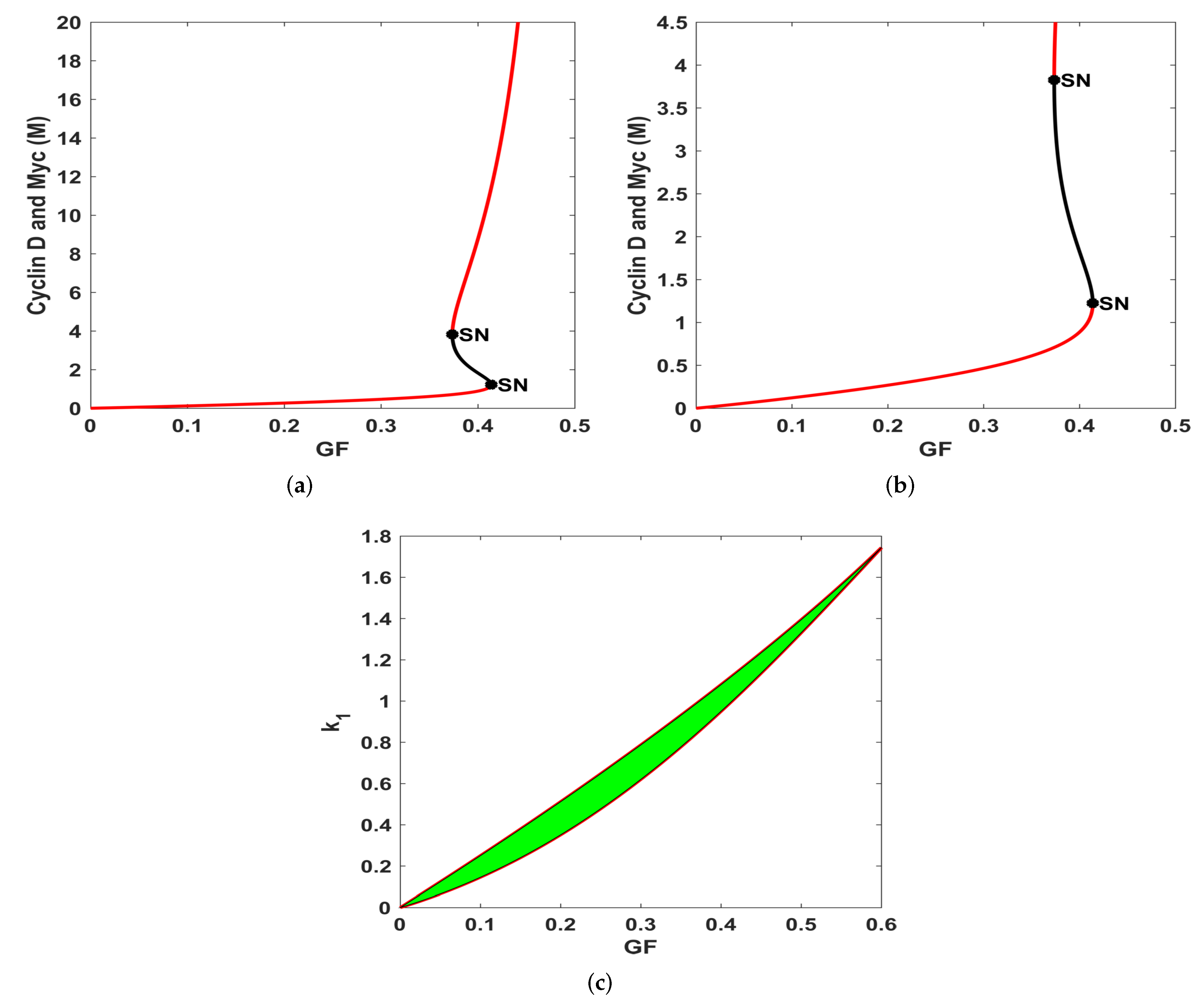
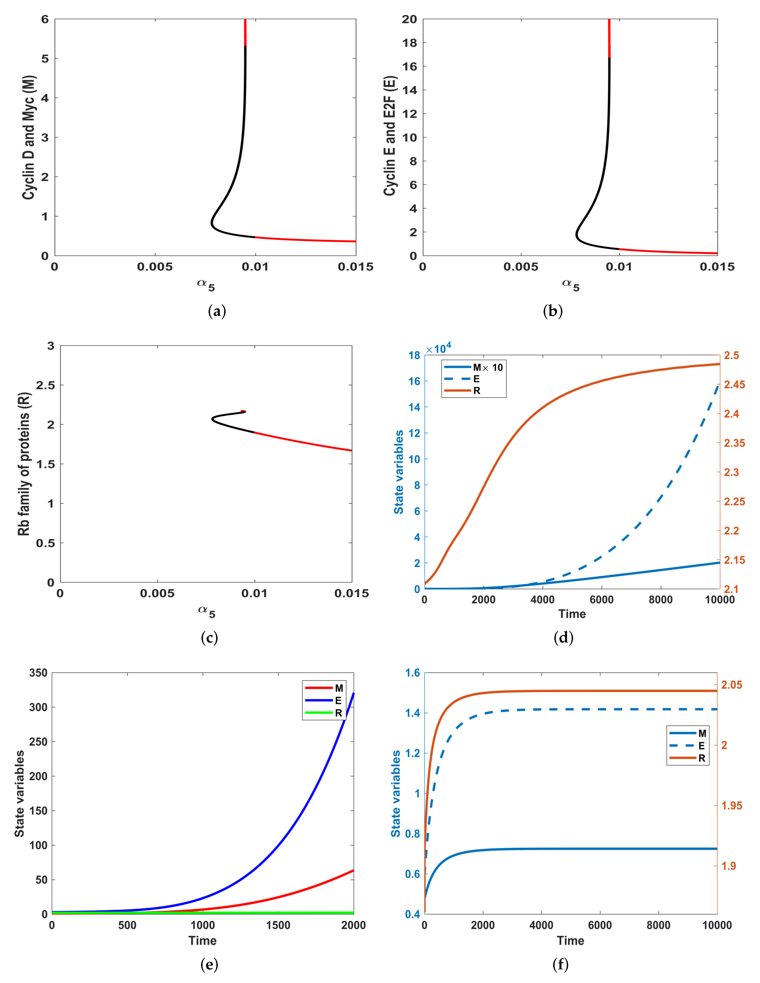
3.1. Bifurcation Analysis

Bifurcation analysis of the system of ODEs (1) was carried out using XPPAUT, a software program freely available from https://asmedigitalcollection.asme.org/appliedmechanicsreviews/article/56/4/B53/463898/Simulating-Analyzing-and-Animating-Dynamical (accessed on 22 November 2020) [53]. Parameter values for our model are shown in Table 1, unless otherwise specified. The parameter values were chosen based on the literature whenever possible and some of them adjusted to illustrate qualitative dynamics [17,42]. As shown in Figure 2a, there exists a unique steady state corresponding to the quiescent state when $GF<0.3735$ with $M^{*}<1.225$. For $0.3735<GF<0.4138$, bistable dynamics result from a saddle node bifurcation marked by two black dots labelled as SN (saddle node). As $GF$ increases further out of the bistable regime, $M^{*}$ jumps into its high steady state, where a cell undergoes proliferation. We also plot $k_1$ against $GF$ and generate a two parameter bifurcation diagram shown in Figure 2c. In the latter figure, the bistable region is coloured green.

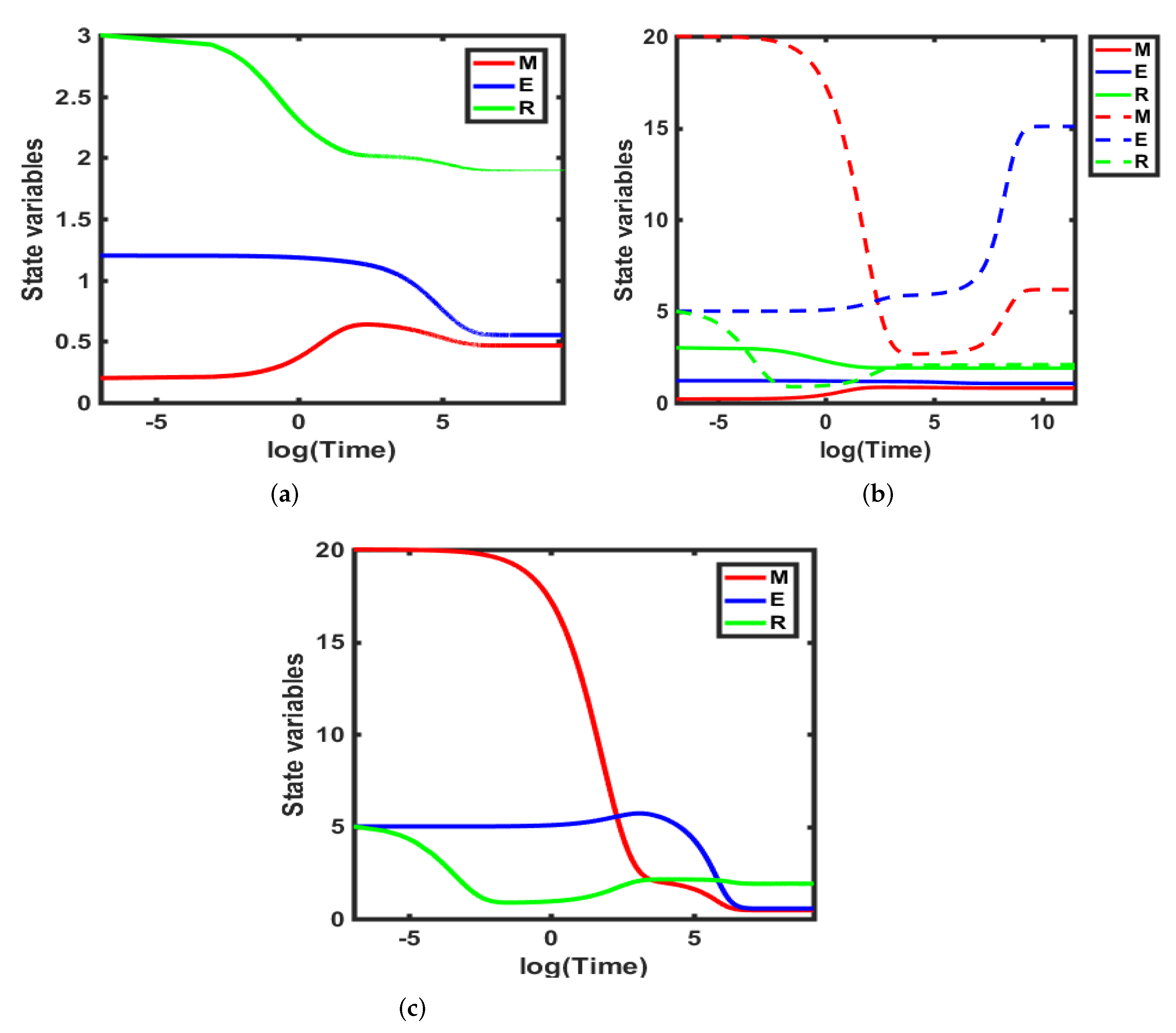
3.2. Numerical Simulations

Numerical simulations were carried out using the MATLAB ode45 solver [54]. This is a standard solver for ordinary differential equations (ODEs) that implements a Runge–Kutta method with a variable time-step for efficient computations, (see [55] for details). We simulated the system by selecting values of $GF$ corresponding to different dynamic regimes deduced through the bifurcation analysis in the previous subsection. We solved the system of ODEs (1) for those three regimes and plot the solution for separate time intervals with a variable growth factor concentration value and for different initial conditions.

First, we show the time evolution for $M\left(t\right)$, $R\left(t\right)$ and $E\left(t\right)$ by solving numerically system (1) with parameters as outlined in Table 1 assuming the growth factor has concentration value $GF=0.3$ with initial conditions $M_0=0.2$, $E_0=1.2$ and $R_0=3$, which bring the system to the lower stable region, as shown in Figure 3a.

Second, we solved the system with the growth factor concentration $GF$ value of $0.39$ and two sets of initial conditions $M_0=0.2$, $E_0=1.2$, $R_0=3$ and $M_0=20$, $E_0=5$, $R_0=5$ while keeping all the other parameters fixed. The results obtained show that the system exhibits bistability, as shown in Figure 3b. Third, we solved the model after adjusting the growth factor concentration $GF$ to $0.45$ and, keeping all other parameters unchanged and initial conditions $M_0=20$, $E_0=5$ and $R_0=5$, the model evolves to a higher steady state, as shown in Figure 3c. These results confirm the conditions set in Theorem 2.

Next, we explored conditions given in Lemma 3 and Theorem 2, as demonstrated in Figure 4. Figure 4 illustrates numerically the dynamics of model system (1) when both Lemma 3 and Theorem 2 are violated. When both conditions of Lemma 3 and Theorem 2 are not satisfied, then there exist two steady states, one stable and another unstable, and, henceforth, the possibility of two different dynamics: either bounded (stable) or unbounded (unstable) solutions. The unstable steady state acts as a switch, determining the initial conditions under which the system may exhibit bounded or unbounded behaviour.

To illustrate such dynamics, we set ${\alpha }_5=0.0079$, $\delta =1$ and $GF=0.3$, while keeping the rest of the parameters fixed, as shown in Table 1. This choice of parameters ensures that conditions (B) and (C) outlined in Theorem 2 are violated while, at the same time, the $min(\theta ,\varphi )=0$, which violates Lemma 3. With this choice of parameters, model system (1) exhibits two steady states, as predicted above, an unstable and a stable steady state, which leads to either unbounded (unstable) or bounded (stable) solutions, respectively. Figure 4d demonstrates the validity of our theoretical results; the system of ODEs (1) becomes unstable with solutions for $M\left(t\right)$ and $E\left(t\right)$ growing unboundedly while those of $R\left(t\right)$ remain bounded. The biological justification for this type of model behaviour lies in our assumptions. Unlike the Rb family of proteins, which are assumed to be conserved for all time, $M\left(t\right)$ and $E\left(t\right)$ species are not conserved, because they are assumed to exist in abundance. Therefore, they are not constrained by laws of mass conservation. We also plot the bifurcation diagram as shown in Figure 4a, for which we have the lower stable steady state shown in red $\left((M^{*},E^{*},R^{*})=(0.7255,1.4184,2.0449)\right.$ with $\left.{\alpha }_5=0.0079\right)$, followed by an upper unstable steady state also for the same parameter value ${\alpha }_5=0.0079$ (shown in grey) $(M^{*},E^{*},R^{*})=(0.9755,2.25168,2.08855).$ For completeness, we have included the bifurcation diagrams for $E\left(t\right)$ and $R\left(t\right)$, respectively, as illustrated in Figure 4b,c. The eigenvalues of the above steady states are given by $(-3.7119,-0.4209,-0.0015)$ and $(-5.6216,-0.3165,0.0013)$, respectively, confirming that the lower steady state is stable while the upper is unstable. The unstable steady state acts as a switch mechanism between the unbounded and bounded solutions, determining the initial conditions under which the system may either exhibit unbounded or bounded solutions when conditions in Lemma 3 and Theorem 2 are violated.

We complete this section by illustrating stable dynamics of model system (1), as shown in Figure 4f. To obtain bounded solutions close to the unstable steady state, we adjusted our initial conditions to $M_0=0.4782$, $E_0=0.594$ and $R_0=1.8616$, such that these are located below the unstable steady state. The model system solved with this set of initial conditions exhibits bounded solutions which converge to the stable steady state computed above.

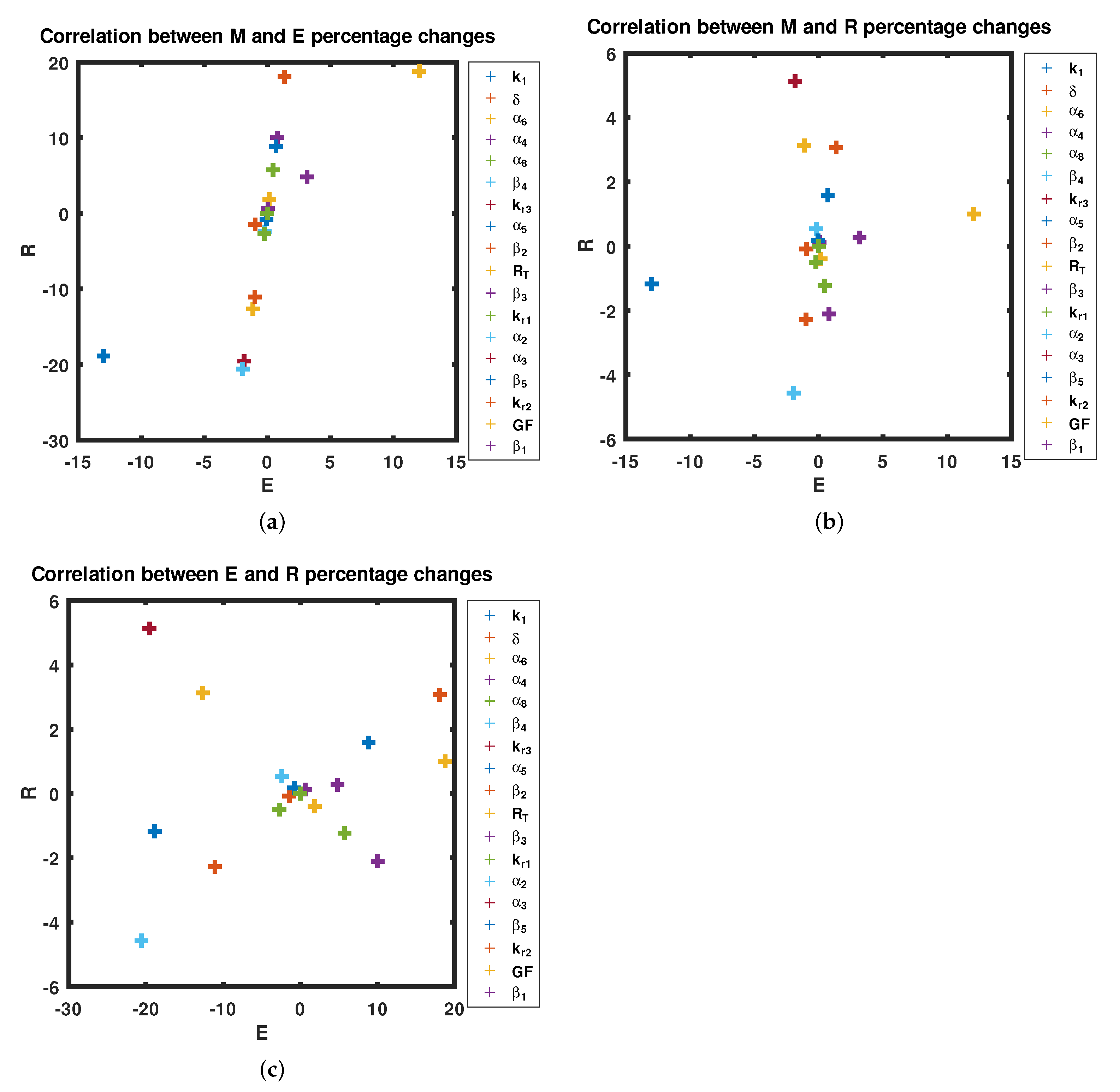
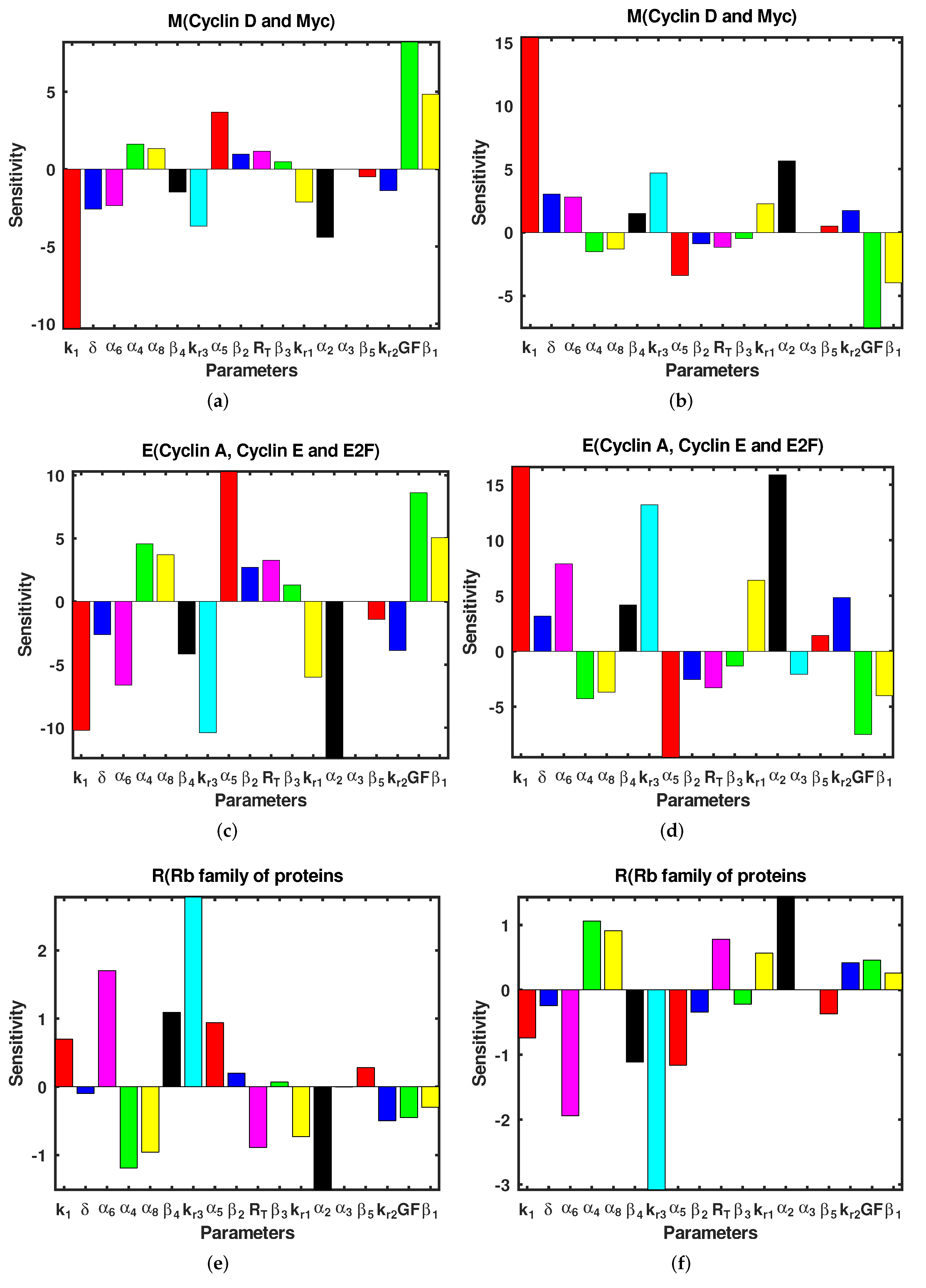
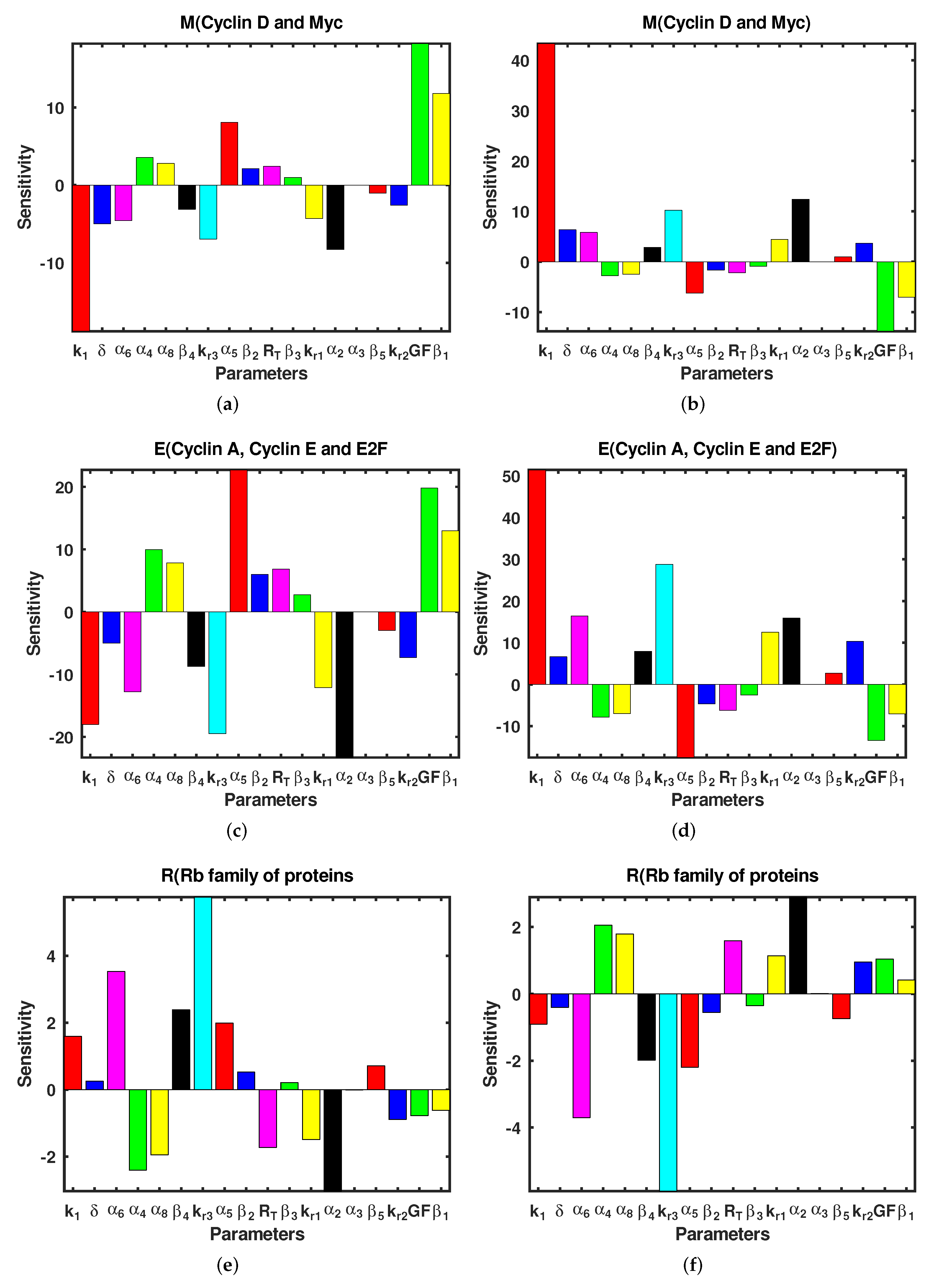
3.3. Sensitivity Analysis

Following the works in [56,57,58], we present the local sensitivity analysis of system (1) with respect to baseline parameter values in Table 1. We used local sensitivity analysis to identify the set of model parameters whose percentage change from the baseline parameter set causes significant changes in the model output [59]. Hence, local sensitivity analysis provides a useful insight into identifying model components that contribute most to the variability in the model output [59,60]. In general, there are two types of sensitivity analyses: local and global. In this article, we focused on local sensitivity analysis, which will allow us to evaluate changes in the model output with respect to variations in a single parameter at a time [59,61]. Global sensitivity analysis will allow for simultaneous changes in model parameters and evaluation of the interaction between parameters, which is not in our interest at this stage. Our methodology involves increasing parameters one at a time by 5%, and 10% and decreasing them by 5% and 10%, respectively. Next, we calculated the local sensitivity indices (percentage changes) in the solutions for $M\left(t\right)$, $E\left(t\right)$ and $R\left(t\right)$. The results for 5% increase, 5% decrease, 10% increase and 10% decrease are shown in

Table 2. Percentage changes in the steady-state values $M^{*}$, $E^{*}$ and $R^{*}$ after a 5% increase in parameter values of the non-linear model (1).

5% Increase in Parameter	% Change in ${\mathit{M}}^{*}$	% Change in ${\mathit{E}}^{*}$	% Change in ${\mathit{R}}^{*}$
$k_1$	−10.330	−10.186	0.7016
$\delta$	−2.5797	−2.6158	−0.0973
${\alpha }_6$	−2.3573	−6.6279	1.7049
${\alpha }_4$	1.6213	4.5563	−1.1907
${\alpha }_8$	1.3212	3.7135	−0.96101
${\beta }_4$	−1.4816	−4.1652	1.0916
$k_{r_3}$	−3.6855	−10.361	2.78
${\alpha }_5$	3.6754	10.331	0.9486
${\beta }_2$	0.9689	2.7222	0.1993
$R_T$	1.1586	3.2559	−0.8912
${\beta }_3$	0.4682	1.3150	0.0671
$k_{r_1}$	−2.1313	−5.9929	−0.73 16
${\alpha }_2$	−4.4144	−12.411	−1.5102
${\alpha }_3$	0.0008	0.00217	−0.0044
${\beta }_5$	−0.50358	−1.4171	0.2834
$k_{r_2}$	−1.3792	−3.8783	−0.5012
$GF$	8.2181	8.6153	−0.4477
${\beta }_1$	4.8355	5.0458	−0.30391

,

Table 3. Percentage changes in the steady-state values $M^{*}$, $E^{*}$ and $R^{*}$ after a 5% decrease in parameter values of the non-linear model (1).

5% Decrease in Parameter	% Change in ${\mathit{M}}^{*}$	% Change in ${\mathit{E}}^{*}$	% Change in ${\mathit{R}}^{*}$
$k_1$	15.379	16.574	−0.74247
$\delta$	3.0549	3.1573	−0.23624
${\alpha }_6$	2.7989	7.8667	−1.9380
${\alpha }_4$	−1.5130	−4.2539	1.0604
${\alpha }_8$	−1.3083	−3.6785	0.91636
${\beta }_4$	1.4856	4.1750	−1.1118
$k_{r_3}$	4.6941	13.194	−3.0811
${\alpha }_5$	−3.3974	−9.5522	−1.1635
${\beta }_2$	−0.90100	−2.5340	−0.34861
$R_T$	−1,1643	−3.2747	0.77670
${\beta }_3$	−0.47058	−1.3243	−0.22096
$k_{r_1}$	2.2750	6.3943	0.56813
${\alpha }_2$	5.6528	15.889	1.4395
${\alpha }_3$	−0.00076	−2.0707	0.00434
${\beta }_5$	0.50506	1.4196	−0.37425
$k_{r_2}$	1.7225	4.8407	0.41722
$GF$	−7.5303	−7.4886	0.46275
${\beta }_1$	−3.9715	−4.0111	0.25848

,

Table 4. Percentage changes in the steady-state values $M^{*}$, $E^{*}$ and $R^{*}$ after a 10% increase in parameter values of the non-linear model (1).

10% Increase in Parameter	% Change in ${\mathit{M}}^{*}$	% Change in ${\mathit{E}}^{*}$	% Change in ${\mathit{R}}^{*}$
$k_1$	−18.792	−18.005	1.5896
$\delta$	−4.9970	−5.0238	0.25366
${\alpha }_6$	−4.5627	−12.828	3.5291
${\alpha }_4$	3.5450	9.9639	−2.4070
${\alpha }_8$	2.7918	7.8469	−1.9470
${\beta }_4$	−3.1078	−8.7368	2.3944
$k_{r_3}$	−6.9382	−19.505	5.7536
${\alpha }_5$	8.0605	22.659	1.9911
${\beta }_2$	2.1256	5.9736	0.52836
$R_T$	2.4269	6.8214	−1.7297
${\beta }_3$	0.9800	2.7539	0.2105
$k_{r_1}$	−4.3112	−12.122	−1.4863
${\alpha }_2$	−8.2964	−23.324	−3.0332
${\alpha }_3$	0.0017	0.0047	−0.0093
${\beta }_5$	−1.0545	−2.9658	0.7076
$k_{r_2}$	−2.6078	−7.3322	−0.8934
$GF$	18.296	19.8	−0.7814
${\beta }_1$	11.815	12.677	−0.6242

and

Table 5. Percentage changes in steady-state values $M^{*}$, $E^{*}$ and $R^{*}$ after a 10% decrease in parameter values of the non-linear model (1).

10% Decrease in Parameter	% Change in ${\mathit{M}}^{*}$	% Change in ${\mathit{E}}^{*}$	% Change in ${\mathit{R}}^{*}$
$k_1$	43.284	51.402	−0.90841
$\delta$	6.340764	6.6298	−0.40674
${\alpha }_6$	5.8216	16.364	−3.7086
${\alpha }_4$	−2.7912	−7.8475	2.0483
${\alpha }_8$	−2.4764	−6.9631	1.7939
${\beta }_4$	2.8264	7.9439	−1.9852
$k_{r_3}$	10.236	28.774	−5.9032
${\alpha }_5$	−6.2295	−17.514	−2.2045
${\beta }_2$	−1.6616	−4.6717	−0.56234
$R_T$	−2.2183	−6.2377	1.5914
${\beta }_3$	−0.89676	−2.5224	−0.34685
$k_{r_1}$	4.44444	12.49	1.1354
${\alpha }_2$	12.394	34.839	2.8958
${\alpha }_3$	−0.0014110	−0.0038423	0.0081792
${\beta }_5$	0.95936	2.6969	−0.73757
$k_{r_2}$	3.6812	10.3 47	0.94703
$GF$	−13.836	−13.470	1.0361
${\beta }_1$	−7.0325	−7.0261	0.41178

, respectively. We proceed to illustrate comparatively the results corresponding to 5% increase and decrease in Figure 5 as well as 10% increase and decrease in Figure 6 for each variable. First, we observe that the steady state $M^{*}$ is mostly sensitive to parameters $k_1$ and $GF$, as shown in Figure 5a,b. Clearly, $k_1$ and $GF$ have negative and positive effects to $M^{*}$, respectively, corresponding to 5% increase and decrease in parameters. This means that increasing $k_1$ reduces $M^{*}$, whereas increasing $GF$ increases $M^{*}$. Second, the steady state $E^{*}$ is mostly sensitive to ${\alpha }_2$ and ${\alpha }_5$ followed by $k_1$, $k_{r_1}$ and $GF$, as shown in Figure 5c,d. Third, $k_{r_3}$ and ${\alpha }_2$ have the greatest effect on $R^{*}$ followed by ${\alpha }_4$ and ${\alpha }_6$, as shown in Figure 5c,d. It is also pertinent to note that the effect of 5% parameter increases on the steady states of $M\left(t\right)$, $E\left(t\right)$ and $R\left(t\right)$ has a direct opposite effect to that of reducing the parameters by the same margin, as shown in Figure 5a–f. Furthermore, the response of $M\left(t\right)$, $E\left(t\right)$ and $R\left(t\right)$ steady-state values to a 5% increase in parameters is almost similar, as shown in Figure 5a,c. In addition, the response of the $M\left(t\right)$, $E\left(t\right)$ and $R\left(t\right)$ steady-state values to a 5% decrease in parameters is also similar, as shown in Figure 5b,d, albeit with different magnitudes.

This can interpreted biologically as follows: increasing (i) the growth factor concentration $GF$, (ii) the activation rate of $M\left(t\right)$, and (iii) the inhibition rate of $E\left(t\right)$ by $R\left(t\right)$ will result in an increase in the steady-state values of $M\left(t\right)$ and $E\left(t\right)$, leading to proliferation. Decreasing these parameters will reduce their respective steady states, leading cells to quiescence. In Figure 5e, all the parameters except ${\alpha }_2$, ${\alpha }_5$, ${\beta }_2$, ${\beta }_3$, $k_{r_1}$, and $k_{r_2}$ have an opposite effect on the steady state of $R\left(t\right)$ when compared to those of $M\left(t\right)$ and $E\left(t\right)$, as shown in Figure 5a,c. Thus, increasing these parameters would have the effect of suppressing both $M^{*}$ and $E^{*}$, as well as increasing $R^{*}$.

Next, we proceed to investigate the correlations between parameter sensitivities to parameter changes for M against E, M against R and E against R, respectively, by considering a 5% increase in parameters. The results are shown in Figure 7. From Figure 7a, it is clear that all parameters except $k_1$, $\delta$, ${\beta }_1$ and $GF$ affect the steady states $M^{*}$ and $E^{*}$ in the same way, since they lie on the same straight line. The parameters $\delta$ and $k_1$ have a negative effect on $M^{*}$, $E^{*}$ and a positive effect on $R^{*}$, i.e., an opposite effect on $R^{*}$. Parameter $GF$ has a positive effect on both $M^{*}$ and $E^{*}$ and an opposing effect on $R^{*}$. In Figure 7b,c, there is almost no correlation between the changes in the steady-state values $M^{*}$ against $R^{*}$ as well as $E^{*}$ against $R^{*}$.

To proceed, we interpret the correlations shown in Figure 7. Generally, the order of the impact of parameters on $M\left(t\right)$ and $E\left(t\right)$ between a $5\%$ and $10\%$ increase in parameters is found to be similar, see Table 2 and Table 4. This fact is also true for 5% and 10% decreases in parameters, as shown in Table 3 and Table 5. This confirmed that none of the parameters of the system has a switching effect; that is, when they reach a particular threshold, their effect on the steady state is greatly increased, in relation to the other parameters. Having identified this, it is inferred that the dynamics of proliferation–quiescence transition remained unaltered with respect to small perturbations in parameters. In Figure 7a, most of the parameters are distributed linearly; thus, these parameters affect both $M\left(t\right)$ and $E\left(t\right)$ solutions in a similar fashion. Both Figure 7b,c show a similar pattern, in which parameter values are grouped in two well correlated sets. The first set contains parameters ${\alpha }_2$, $k_{r_1}$, $k_{r_2}$, ${\beta }_3$, ${\beta }_2$ and ${\alpha }_5$, while the other contains $k_{r_3}$, ${\alpha }_6$, ${\beta }_4$, ${\alpha }_3$, $R_T$, ${\alpha }_4$ and ${\alpha }_8$. The effects of changes in ${\alpha }_3$ are absolutely negligible, as shown in Figure 5 and Figure 6. Biologically, ${\alpha }_3$ represents the inhibition rate of R by E which is a two-stage process involving the dephosphorylation of the Rb family of proteins [40] followed by the inhibition of these proteins. This effectively means that the inhibition process depends on the dephosphorylation of the Rb family of proteins, thus explaining the negligible sensitivity observed in this case. The parameter $\delta$ lies off the linear pattern, as shown in Figure 7a, which is a result of its role in the proliferation–quiescence transition. It is known that variation in cyclin D levels through the cell cycle determines the proliferating fate of a cell [40]. Parameters $\delta$, $k_1$, ${\alpha }_1$ and $GF$ lie off the well-defined linear pattern followed by the rest of the parameters. From this observation, it is inferred that a $10\%$ increase in the inhibition rate of M (Cyclin D and Myc) causes a significant decrease in the activation of $E\left(t\right)$ (E2F, Cyclin E, Cyclin A) and a small increase in the activation of the $Rb$ family of proteins. Under these circumstances, cells would naturally enter the quiescence state. Additionally, an increase in the expression of the $Rb$ family of proteins significantly reduces the expression levels of E (E2F, Cyclin E and Cyclin A), thereby preventing cells from entering the cell cycle.

4. Discussion

Biologically, it was shown that the growth factor concentration plays a pivotal role in a wide range of cellular processes, including cellular growth and differentiation [40]. As such, growth factor (GF) stimulation has a profound effect on cancer development [18,19,21]. Previous studies have shown that the $Rb-E2F$ bistable switch converts graded and transient serum growth signals into a binary and hysteric $E2F$ activity in individual cells [2].

In this paper

• Based on the concept of first principles, we investigated the dynamical potential of growth factors in the regulation of the cell-cycle entry.
• A mathematical model for the simplified $Rb-E2F$ network was constructed based on the model proposed in Yao et al. [2]. While previous studies modelled all links using Michaelis–Menten functions only [2], we used mass action, and Michaelis–Menten and Hill functions, resulting in a simpler model. In addition, we considered the R species to exist either in hyper-phosphorylated or hypo-phosphorylated form and that their total concentration is conserved.
• By varying the growth factor signal values through bifurcation analysis, numerical simulations illustrated that the magnitude of the value of the growth factor plays a critical role in regulating cell-cycle entry. Through bifurcation analysis, we deduced the existence of three consecutive dynamical behaviours, namely, stability, bi-stability and stability.
• Numerical simulations performed with different growth factor values validated the results derived from the bifurcation analysis. In particular, the biological interpretation of the uniform steady state can be established as follows:
  • For $GF<0.3735$, System (1) is asymptotically stable, indicating the regime in which cells are in a quiescent state. In this state, cells feature low levels of Cyclin D, Myc and high levels of R species.
  • On the other hand, in the range $0.3735<GF<0.4138$, System (1) exhibits bi-stability, marking the position of the restriction point, as deduced in Yao et al. [42]. This point sets a high threshold separating quiescence from proliferation and acts as a barrier against unregulated and accidental cell growth. In addition, it provides a low-maintenance mechanism ensuring that the cell cycle proceeds, albeit later due to changes in the extracellular environment which is crucial for maintaining genome integrity.
  • For values of $GF>0.4138$, the system generates a stable dynamical behaviour where a cell is in the proliferation mode marking the higher steady state value. This state features high levels of Cyclin D, Myc and low levels of the $Rb$ family of proteins.
  However, it remains to investigate the conditions under which the system exhibits excitable and oscillatory dynamics as observed in a different model proposed in [62], but that would be investigated in a subsequent work. While Yao et al. [42] identified a basic gene circuit underlying resettable $Rb-E2F$ bi-stable switch controlling cell-cycle entry, we obtained a range of values of the growth factor concentration for the three dynamical regimes.

In this study, we focused our attention on the quantitative aspects of bi-stability, including ascertaining some constraints and the region for bi-stability, whereas, in [42], the focus was on the qualitative aspects of bi-stability.

Our consideration of the conservation of the R species did not affect the bistable nature of the system but revealed that the system becomes unstable at very low levels of the concentration of the R species. Local sensitivity analysis revealed that increasing parameters that enhance the availability of Cyclin A, Cyclin E, Cyclin D, Myc and E2F in the model results in the hyper-phosphorylation of Rb proteins. In its hyper-phosphorylated state, the Rb loses its affinity to bind free E2F, which results in transcription, leading to proliferation [40]. On the contrary, reducing these parameters by a small margin results in Rb dephosphorylation, which increases its affinity for E2F. Naturally, in its hypo-phosphorylated state, Rb binds to free E2F, impairing transcription. This results in cells being unable to pass through the restriction point and, hence, remaining in quiescence.

5. Limitations

In this study, we constructed an activator-inhibitor model to describe the $Rb-E2F$ signalling interaction network and analysed its dynamics and biological implications. However, in our study there are some limitations. Firstly, the model does not seem to exhibit periodicity and excitable dynamics. Secondly, spatial localisation of the proteins was completely ignored. This will give rise to partial differential equations. Thirdly, we did not fit the model to data to infer model parameters; this forms part of our future studies. Though simplification of the model produced the interesting bistable behaviour consistent with experimental observations, there were consequences on other dynamics of the $Rb-E2F$ signalling network such as oscillatory dynamics, as observed in [62]. Moreover, we assumed that all proteins other than the $Rb$ family of proteins exist in abundance which may not be the case and hence must be investigated in future studies.

References

1. Wang, X.; Fujimaki, K.; Mitchell, G.C.; Kwon, J.S.; Croce, K.D.; Langsdorf, C.; Zhang, H.H.; Yao, G. Exit from quiescence displays a memory of cell growth and division. Nat. Commun. 2017, 8, 321. [Google Scholar] [CrossRef] [PubMed] [Green Version]
2. Yao, G. Modelling mammalian cellular quiescence. Interface Focus 2014, 4, 20130074. [Google Scholar] [CrossRef] [PubMed] [Green Version]
3. Harashima, H.; Dissmeyer, N.; Schnittger, A. Cell cycle control across the eukaryotic kingdom. Trends Cell Biol. 2013, 23, 345–356. [Google Scholar] [CrossRef] [PubMed]
4. Miller, A.K.; Munger, K.; Adler, F.R. A mathematical model of cell cycle dysregulation due to human papilloma virus infection. Bull. Math. Biol. 2017, 79, 1564–1585. [Google Scholar] [CrossRef]
5. Hartwell, L.H.; Weinert, T.A. Checkpoints: Controls that ensure the order of cell cycle events. Science 1989, 246, 629–634. [Google Scholar] [CrossRef] [Green Version]
6. Kastan, M.B.; Bartek, J. Cell-cycle checkpoints and cancer. Nature 2004, 432, 316–323. [Google Scholar] [CrossRef]
7. Naetar, N.; Soundarapian, V.; Litovchick, L.; Goguen, K.L.; Sablina, A.A.; Bowman-Colin, C.; Sicinski, P.; Hahn, W.C.; DeCaprio, J.A.; Livingstone, D.M. PP2A-mediated regulation of Ras signaling in G2 is essential for stable quiescence and normal G1 length. Mol. Cell 2014, 54, 932–945. [Google Scholar] [CrossRef] [Green Version]
8. Nasmyth, K. Viewpoint: Putting the cell cycle in order. Science 1996, 274, 1643–1645. [Google Scholar] [CrossRef]
9. Pardee, A.B. A restriction point for control of normal cell proliferation. Proc. Natl. Acad. Sci. USA 1974, 71, 1286–1290. [Google Scholar] [CrossRef] [Green Version]
10. Qu, Z.; Weiss, J.N.; Maclellan, R. Regulation of mammalian cell cycle: A model of the G1-to-S transition. J. Physiol. Cell Physiol. 2003, 284, C349–C364. [Google Scholar] [CrossRef] [Green Version]
11. Weinberg, R. The Biology of Cancer. In Garland Science; WW Norton & Company: New York, NY, USA, 2013; ISBN 978-0815342205. [Google Scholar]
12. Zetterberg, A.; Larsson, O. Kinetic analysis of regulatory events in G1 leading to proliferation or quiescence of Swiss 3T3 cells. Proc. Natl. Acad. Sci. USA 1985, 82, 5365–5369. [Google Scholar] [CrossRef] [PubMed] [Green Version]
13. Pandey, N.; Vinod, P.K. Mathematical modeling of reversible transition between quiescence and proliferation. PLoS ONE 2018, 13, e0198420. [Google Scholar] [CrossRef] [PubMed]
14. Chen, H.Z.; Tsai, S.Y.; Leone, G. Emerging roles of E2Fs in cancer: An exit from cell cycle control. Nat. Rev. Cancer 2009, 9, 785–797. [Google Scholar] [CrossRef] [PubMed] [Green Version]
15. Nevins, J.R. The Rb/E2F and cancer. Hum. Mol. Genet 2001, 10, 699–703. [Google Scholar] [CrossRef]
16. Nevins, J.R. E2F: A link between the Rb tumor suppressor protein and viral oncoproteins. Science 1992, 258, 424–429. [Google Scholar] [CrossRef]
17. Yao, G.; Lee, T.J.; Mori, S.; Nevins, J.R.; You, L. A bistable Rb-E2F switch underlies the restriction point. Nat. Cell Biol. 2008, 10, 476–482. [Google Scholar] [CrossRef]
18. Burns, F.J.; Tannock, I.F. On existence of a G0-phase in cell cycle. Cell Tissue Kinet. 1970, 3, 321. [Google Scholar]
19. De Maertelaer, V.; Galand, P. Some properties of a “G0” -model of the cell cycle. II. Natural constraints on the theoretical model in exponential growth conditions. Cell Tissue Kinet. 1975, 8, 11–22. [Google Scholar] [CrossRef]
20. Shields, R.; Smith, J.A. Cells regulate their proliferation through alterations in transition probability. J. Cell. Physiol. 1977, 91, 345–355. [Google Scholar] [CrossRef]
21. Smith, J.A.; Martin, L. Do cells cycle? Proc. Natl Acad. Sci. USA 1973, 70, 1263–1267. [Google Scholar] [CrossRef] [Green Version]
22. Castor, L.N. A G1 rate model accounts for cell cycle kinetics attributed to transition probability. Nature 1980, 287, 857–859. [Google Scholar] [CrossRef] [PubMed]
23. Koch, A.L. Does the variability of cell cycle result from one or many chance events? Nature 1980, 286, 80–82. [Google Scholar] [CrossRef] [PubMed]
24. Friend, S.H.; Bernards, R.; Rogelj, S.; Weinberg, R.A.; Rapaport, J.M.; Albert, D.M.; Drtja, T.P. A human DNA segment with properties of the gene that predisposes to retinobalstoma and osteosarcoma. Nature 2004, 323, 643–646. [Google Scholar] [CrossRef] [PubMed]
25. Tyson, J.J.; Chen, K.C.; Novak, B. Sniffers, buzzers, toggles and blinkers: Dynamics of regulatory and signaling pathways in the cell. Curr. Opin. Cell. Biol. 2003, 15, 221–231. [Google Scholar] [CrossRef]
26. Aguda, B.D.; Tang, Y. The kinetic origins of the restriction point in the mammalian cell cycle. Cell Prolif. 1999, 32, 321–335. [Google Scholar] [CrossRef] [PubMed]
27. Gardner, T.S.; Dolnik, M.; Collins, J.J. A theory for controlling cell cycle dynamics using a reversibility binding inhibitor. Proc. Natl. Acad. Sci. USA 1998, 95, 14190–14195. [Google Scholar] [CrossRef] [Green Version]
28. Goldbeter, A. A minimal cascade model for the mitotic oscillator involving cyclin and cdc kinase. Proc. Natl. Acad. Sci. USA 1991, 88, 9107–9111. [Google Scholar] [CrossRef] [Green Version]
29. Kohn, K.W. Functional capabilities of molecular network components controlling the mammalian G1/S cell cycle phase transition. Oncogene 1998, 16, 1065–1075. [Google Scholar] [CrossRef] [Green Version]
30. Norel, R.; Agur, Z. A model for the adjustment of the mitotic clock by cyclin and MPF levels. Science 1991, 251, 1076–1078. [Google Scholar] [CrossRef]
31. Nurse, P. The incredible life and times of biological cells. Science 2000, 289, 1711–1716. [Google Scholar] [CrossRef] [Green Version]
32. Obeyesekere, M.N.; Knudsen, E.S.; Wang, J.Y.J.; Zimmernan, S.O. A mathematical model of the regulation of the G1 phase of Rb+/+ and Rb−/− mouse embryonic fibroblasts and an osteosarcoma cell line. Cell Prolif. 1997, 30, 171–194. [Google Scholar] [CrossRef] [PubMed]
33. Thron, C.D. Bistable biochemical switching and the control of the events of cell cycle. Oncogene 1997, 15, 317–325. [Google Scholar] [CrossRef] [PubMed] [Green Version]
34. Tyson, J.J.; Novak, B. Regulation of the eukaryotic cell: Molecular antagonism hysteresis, and irreversible transitions. J. Theor. Biol. 2001, 210, 249–263. [Google Scholar] [CrossRef] [Green Version]
35. Tyson, J.J.; Novak, B. Checkpoints in the cell cycle from modeler’s perspective. Prog. Cell Cycle Res. 1995, 1, 1–8. [Google Scholar] [CrossRef] [PubMed]
36. Novak, B.; Tyson, J.J. Modeling the control of DNA replication in fission yeast. Proc. Natl. Acad. Sci. USA 1997, 94, 9147–9152. [Google Scholar] [CrossRef] [Green Version]
37. Thron, C.D. A model for a bistable biochemical trigger of mitosis. Biophys. Chem. 1996, 57, 239–251. [Google Scholar] [CrossRef]
38. Aguda, B.D. A quantitative analysis of the kinetics of the G2 DNA damage checkpoint system. Proc. Natl. Acad. Sci. USA 1999, 96, 11352–11357. [Google Scholar] [CrossRef] [PubMed] [Green Version]
39. Frolov, M.V.; Dyson, N.J. Molecular mechanisms of E2F-dependent activation and pRB-mediated repression. J. Cell Sci. 2004, 117, 2173–2181. [Google Scholar] [CrossRef] [Green Version]
40. Heldt, F.S.; Barr, A.R.; Cooper, S.; Bakal, C.; Novak, B. A comprehensive model for the proliferation-quiescence decision in response to endogenous DNA damage in human cells. Proc. Natl. Acad. Sci. USA 2017, 115, 2532–2537. [Google Scholar] [CrossRef] [Green Version]
41. Attwooll, C.; Denchi, E.L.; Helin, K. The E2F family: Specific functions and overlapping interests. EMBO J. 2004, 23, 4709–4716. [Google Scholar] [CrossRef]
42. Yao, G.; Tan, C.; West, N.; Nevins, J.T.; You, L. Origin of bistability underlying mammalian cell cycle entry. Mol. Syst. Biol. 2011, 7, 485. [Google Scholar] [CrossRef] [PubMed]
43. Blagosklonny, M.V.; Pardee, A.B. The restriction point of the cell cycle. Cell Cycle 2002, 1, 103–110. [Google Scholar] [CrossRef] [Green Version]
44. Gierer, A.; Meinhardt, H.A. A theory of biological pattern formation. Kybernetik 1972, 12, 30–39. [Google Scholar] [CrossRef] [PubMed] [Green Version]
45. Kamps, D.; Koch, J.; Juma, V.O.; Campillo-Funollet, E.; Graessl, M.; Banerjee, S.; Mazel, T.; Chen, X.; Wu, Y.; Portet, S.; et al. Optogenetic Tuning Reveals Rho Amplification-Dependent Dynamics of a Cell Contraction Signal Network. Cell Rep. 2020, 33, 108467. [Google Scholar] [CrossRef] [PubMed]
46. Sears, R.C.; Nevins, J.R. Signaling network that link cell proliferation and cell fate. J. Biol. Chem. 2002, 277, 11617–11620. [Google Scholar] [CrossRef] [PubMed] [Green Version]
47. Alon, U. An Introduction to Systems Biology: Design Principles of Biological Circuits; Chapman and Hall/CRC: New York, NY, USA, 2006; ISBN 9781439837177. [Google Scholar]
48. Michaelis, L.; Menten, M.L. Die Kinetik der Invertinwirkung. Biochem. Z. 1913, 49, 333–369. [Google Scholar]
49. Murray, J.D. Mathematical Biology I: An Introduction of Interdisciplinary Applied Mathematics; Springer: New York, NY, USA, 2002; pp. 257–271. [Google Scholar]
50. Henley, A.S.; Dick, F.A. The retinoblsatoma family of proteins and their regulatory functions in the mammalian cell division cycle. Cell Div. 2012, 7, 1–14. [Google Scholar] [CrossRef] [Green Version]
51. Hsu, S.-B. Ordinary Differential Equations with Applications, 2nd ed.; National Hua University: Hsinchu, Taiwan, 2013; ISBN 978-981-4452-92-2. [Google Scholar]
52. Fine, B.; Rosenberger, G. The Fundamental Theorem of Algebra; Springer: New York, NY, USA, 1997. [Google Scholar]
53. Ermentrout, B. Simulating, Analyzing, and Animating Dynamical Systems: A Guide to XPPAUT for Researchers and Students; SIAM: Philadelphia, PA, USA, 2002; ISBN 978-0-89971-506-4. [Google Scholar]
54. Shampine, L.F.; Reichdt, M.W. MATLAB ODE Suite. SIAM J. Sci. Comp. 1997, 18, 1–22. [Google Scholar] [CrossRef] [Green Version]
55. Dormand, J.R.; Prince, P.J. A family of embedded Runge-Kutta formulae. J. Comp. Appl. Math. 1980, 6, 19–26. [Google Scholar] [CrossRef] [Green Version]
56. Juma, V.O. Data-Driven Mathematical Modeling and Simulations of Rho-Myosin Dynamics. Ph.D. Thesis, University of Sussex, Sussex, UK, 2019. [Google Scholar]
57. Juma, V.O.; Dehmelt, L.; Portet, S.; Madzvamuse, A. A mathematical analysis of an activator-inhibitor Rho GTPase model. J. Comput. Dyn. 2021, 9, 133. [Google Scholar] [CrossRef]
58. Zagkos, L.; Mc Auley, M.; Roberts, J.; Kavallaris, N.I. Mathematical models of DNA methylation dynamics: Implications for health and ageing. J. Theor. Biol. 2019, 462, 184–193. [Google Scholar] [CrossRef] [PubMed] [Green Version]
59. Zhang, X.-J.; Trame, M.N.; Lesko, L.J.; Schmidt, S. Sobol sensitivity analysis: A tool to guide the development and evaluation of systems phamacology models. CPT Pharmacomet. Syst. Pharmacol. 2015, 4, 69–79. [Google Scholar] [CrossRef] [PubMed]
60. Saltelli, A.; Chan, K.; Scott, E.M. Sensitivity Analysis: Wiley Series in Probability and Statistics; Jon Wiley: Chichester, UK, 2000; ISBN 978-0-470-74382-9. [Google Scholar]
61. Hampy, D.M. A review of techniques for parameter sensitivity analysis of environmental models. Environ. Monit. Assess. 1994, 32, 135–154. [Google Scholar] [CrossRef] [PubMed]
62. Yan, F.; Liu, H.; Hao, J.; Liu, Z. Dynamical behaviors of RBE2F pathway including negative feedback loops involving miR449. PLoS ONE 2012, 7, e43908. [Google Scholar] [CrossRef]
Figure 1. An activator-inhibitor network for the R b E 2 F signalling network [42]. The solid arrows represent activation mechanism while the broken lines represent inhibition. Here, the growth factors G F activate M (cyclin D and M y c ) and, in turn M activates E (cyclin A , cyclin E and E 2 F transcription factors) while E activates M, forming a positive feedback loop. R ( R b family of proteins) inhibits E, while E activates and inhibits R and M inhibits R.
Mathematics 10 02426 g001
Figure 2. Numerical bifurcation diagrams for the system of ODEs (1), with parameter values listed in Table 1. (a) One parameter bifurcation diagram for M * , with the growth factor G F concentration value as a bifurcation parameter. The saddle-node (SN) bifurcation points for G F are 0.3735 and 0.4138 and the corresponding M * are 3.826 and 1.225, respectively. The red line represents the stable steady states whereas the thin black line represent saddle points. The black dots labelled SN are the saddle-node bifurcation points, which span the region characterised by bistable dynamics. (b) A one-parameter bifurcation diagram showing a zoom of (a) around the two saddle-node bifurcation points. (c) Two-parameter bifurcation diagram with k 1 and G F as bifurcation parameters. The green coloured region is characterised by bistable dynamics, whereas the colourless region is characterised by stable dynamics.
Mathematics 10 02426 g002
Figure 3. Numerical simulations illustrating the time evolution dynamics of ( M ( t ) , R ( t ) , E ( t ) ) for system (1) corresponding to different dynamic regimes. As the value of G F increases, the system transitions from stable ((a) with G F = 0.3 and initial conditions M 0 = 0.2 , E 0 = 1.2 , R 0 = 3 ) through bistable ((b) with G F = 0.39 and two sets of initial conditions M 0 = 0.2 , E 0 = 1.2 , R 0 = 3 and M 0 = 20 , E 0 = 5 and R 0 = 5 ) then back to stable ((c) with G F = 0.45 and initial conditions M 0 = 20 , E 0 = 5 and R 0 = 5 ).
Mathematics 10 02426 g003
Figure 4. Numerical bifurcations and simulations illustrating the dynamics of System (1) where we explore the conditions of Theorem 2. (ac) bifurcation diagrams for M ( t ) , E ( t ) and R ( t ) , respectively, with respect to α 5 ; other parameter values are fixed as shown in Table 1 and G F = 0.3 . (d) shows unbounded solutions of E and M with α 5 = 0.0079 , δ = 1 and G F = 0.3 , while keeping all the other parameters fixed as in Table 1 and initial conditions M 0 = 1.2 , E 0 = 3 , R 0 = 1.2 so that the conditions set in Theorem 2 and 3 are not met. To be more specific, γ 2 > 0 , which is against conditions (A), (B) and (C) of Theorem 2. The M ( t ) curve was amplified by a factor of 10 to visualize its behaviour with time and show that it grows unbounded with time while the R curve remain bounded because of conservation. (e) illustrates a zoom of the unstable dynamics of (d) for a short time t [ 0 , 2000 ] without scaling. (f) shows the stable time evolution of M ( t ) , E ( t ) and R ( t ) with α 5 = 0.0079 , δ = 1 and G F = 0.3 with initial condition ( M 0 , E 0 , R 0 ) = (0.4782, 0.594, 1.8616). With these parameters, the model converges to the steady state ( M * , E * , R * ) = (0.7255, 1.4184, 2.0449).
Mathematics 10 02426 g004
Figure 5. Parameter sensitivities for system (1) corresponding to 5% increase and decrease in parameters. (a,b) show sensitivity of M * after 5 % increase and decrease in parameters, respectively; (c,d) show sensitivity of E * corresponding to 5% increase and decrease, respectively. (e,f) show sensitivity R * to 5% increase and decrease in parameters, respectively.
Mathematics 10 02426 g005
Figure 6. Parameter sensitivities for system (1) corresponding to 10% increases and decrease in parameters. (a,b) show sensitivity of M * after 10 % increase and decrease in parameters, respectively, (c,d) show sensitivity of E * corresponding to 10% increases and decrease, respectively. (e,f) show sensitivity R * to 10% increases and decrease in parameters, respectively.
Mathematics 10 02426 g006
Figure 7. Correlation between parameter sensitivity of M ( t ) , E ( t ) and R ( t ) corresponding to 10 % increase in model parameters. (a) shows the correction between M ( t ) and E ( t ) , (b) shows the correlation between M ( t ) and R ( t ) and (c) shows the correlation between E ( t ) and R ( t ) .
Mathematics 10 02426 g007