A Discrete Representation of the Second Fundamental Form

Abstract

We present a new method to obtain a combinatorial representation for the behaviour of a submanifold isometrically immersed in a Riemannian manifold based on the second fundamental form. We also present several results applying this new way of representation.

1. Introduction

Linking different branches of mathematics has always been a very interesting way of approaching problems due to the tools provided by both sides. Some examples of linking differential geometry with graph theory can be found in [1,2], where the authors present a representation of vector spaces of even dimension and submanifolds with combinatorial structures. All of them have obtained nice results in their areas.

When we study a submanifold isometrically immersed in a Riemannian manifold $(\tilde{M},g)$, it is very important to take into account its behaviour with respect to the second fundamental form. Many submanifolds presenting homogeneus behaviour in this sense have been defined: totally geodesic submanifolds, minimal submanifolds, totally umbilical submanifolds and so forth. Most of them have something in common, and they can be characterized by a certain combinatorial structure described in this paper. The idea of this combinatorial structure is influenced by [3], where the author introduced a graphic representation of submanifolds in order to understand the behaviour of a submanifold with respect to the almost-complex structure.

In fact, we present a new method of submanifold representation by a combinatorial structure in order to understand the behaviour of the second fundamental form. This representation is closely related to a selected local frame field of tangent vector fields, and it depends on it. Thus, it will be more useful in the case of the existence of special local frame fields, for instance, when the ambient Riemannian manifold has an extra structure. On the other hand, sometimes, it is possible to obtain information about the submanifold by using the representation.

The paper is organized as follows. After a general preliminaries section, in which we recall some definitions and results for later use, in Section 3, we define the new representation and present some examples in which we point out the dependence on the selected local frame field, and we see how to obtain information of the submanifold from such a representation. In Section 4, we study some general results concerning this representation; specifically, we characterize totally umbilical submanifolds by using it. In Section 5, we study a Lagrangian submanifold of Kaehler manifolds, in which there exists a distinguished local frame field, and we prove a pure differential geometry theorem (Theorem 3) from the obtained results. Finally, we show other utilities that the representation can have with a well-known example: the Clifford torus.

2. Preliminaries

In this section, we recall some general definitions and basic formulas which we will use later. For more background on the geometry of submanifolds, we recommend the references [4,5]. We will recall some more specific notions and results in the following sections, when needed.

From now on, let M be an isometrically immersed m-dimensional submanifold of a n-dimensional Riemannian manifold $(\tilde{M},g)$, and let us denote by ∇ and $\tilde{\nabla }$ their respective Levi–Civita connections. Then, the second fundamental form(SFF) is defined as

$$h(X,Y)={({\tilde{\nabla }}_{\tilde{X}}\tilde{Y})}^{\perp },\mathrm{for}\mathrm{any}X,Y\in \mathfrak{X}\left(M\right),$$

where $\tilde{X},\tilde{Y}\in \mathfrak{X}(\tilde{M})$ are the extensions of $X,Y$, respectively. From the Gauss formula, given a local frame field $\mathcal{B}=\{X_1,\cdots X_n\}$ of tangent vector fields to $\tilde{M}$, where the first m vector fields are tangent to M and the last $n-m$ ones are normal to M, the SFF can be written as

$${\displaystyle h(X_i,X_j)=\sum _{k=m+1}^n{h}_{ij}^k{X}_k,i,j=1,\cdots ,m,}$$

where $h_{ij}^k=g(h(X_i,X_j),X_k)$. In addition, for each normal vector field to M, V, the shape operator$A_V$ is the (1,1)-tensor field on M such that $g(X,A_{V}Y)=g(V,h(X,Y)),$ for any $X,Y\in \mathfrak{X}\left(M\right)$.

From the behaviour of the SFF, some types of submanifolds can be defined. In this context, we would like to point out that a submanifold M is called totally geodesic if the SFF vanishes identically, and it is called minimal if the mean curvature vector field,

$${\displaystyle H=\frac{1}{m}\sum _{i=1}^{m}h(X_i,X_i),}$$

vanishes. Moreover, if for each normal vector field $V\in T{M}^{\perp }$, the eigenvalues of $A_V$, ${\lambda }_1,\cdots ,{\lambda }_m$, are invariant under multiplication by $-1$, that is if

$$({\lambda }_1,\cdots ,{\lambda }_m)=(a,-a,b,-b,\cdots ,c,-c,0,\cdots ,0),$$

the submanifold is called austere (see [6] for more details concerning this type of submanifolds). Finally, M is called totally umbilical if $h(X,Y)=g(X,Y)·H$ for any tangent vector fields $X,Y\in \mathfrak{X}\left(M\right)$.

Next, suppose that $\tilde{M}$ is of even dimension. A (1,1)-tensor field J on M is called an almost-complex structure on M if, at every point x on M, J is an endomorphism of the tangent space $T_x\left(M\right)$ such that $J^2=-I$. A manifold M with a fixed almost complex structure J is called an almost-complex manifold. A Hermitian metric on $\tilde{M}$ is a Riemannian metric g such that $g(JX,JY)=g(X,Y)$ for any $X,Y\in \mathfrak{X}(\tilde{M})$. An almost complex manifold with a Hermitian metric is called an almost-Hermitian manifold. An almost-Hermitian manifold is called a Kaehler manifold if its almost complex structure is normal (that is, its Nijenhuis tensor field vanishes) and $\tilde{\nabla }J=0$.

A submanifold M of an almost-Hermitian manifold $(\tilde{M},J,g)$ is called totally real if $J\left(\mathfrak{X}\left(M\right)\right)\subseteq T{M}^{\perp }$ [7]. Furthermore, if $dim(\tilde{M})=2dim\left(M\right)$, then M is called a Lagrangian submanifold. For a m-dimensional Lagrangian submanifold M in $\tilde{M}$, a local orthonormal frame field of tangent vector fields to $\tilde{M}$

$$\{X_1,\cdots ,X_m,X_1^{\prime },\cdots ,X_m^{\prime }\}$$

is called an adapted Lagrangian frame field if $X_1,\cdots ,X_m$ are tangent vector fields to M and $X_1^{\prime },\cdots ,X_m^{\prime }$ are normal vector fields given by $X_i^{\prime }=J{X}_i$, $i=1,\cdots ,m$.

3. A New Submanifold Representation

Let $(\tilde{M},g)$ be a n-dimensional Riemannian manifold and M be an isometrically immersed m-dimensional submanifold. We now introduce a combinatorial representation procedure in order to understand the behaviour of the SFF of the immersion. We follow these steps:

• Let us choose a local orthonormal frame of tangent vector fields to $\tilde{M}$,

  $$\mathcal{B}=\{X_1,\cdots ,X_n\},$$

  such that $X_1,\cdots X_m$ are tangent to M and $X_{m+1},\cdots X_n$ are normal to M.
• We consider a vertex for every field of $\mathcal{B}$, labeled with its corresponding natural index.
• For $i,j\in \{1,\cdots ,m\}$ with $i\le j$ and $k\in \{m+1,\cdots ,n\}$ we have:

  (a)

  If $i=j$, we say that the $\{i,k\}$ edge exists if and only if $h_{ii}^k\ne 0$.

  (b)

  If $i\ne j$, we say that the $\{i,j,k\}$ triangle exists if and only if $h_{ij}^k\ne 0$.

• We assign to every edge $\{i,k\}$ the weight given by $h_{ii}^k$ and on every triangle $\{i,j,k\}$ the weight given by $h_{ij}^k$.
• Finally, notice that we obtain additional visual information by putting the vertices corresponding to tangent fields at an imaginary bottom line and those which correspond to normal fields at a top line.

We are going to use this method with the following examples. For them, let M be a surface isometrically immersed in a Riemannian 4-dimensional manifold $(\tilde{M},g)$.

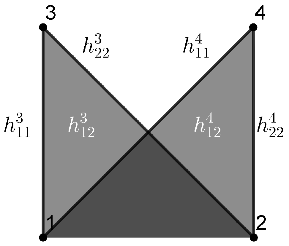
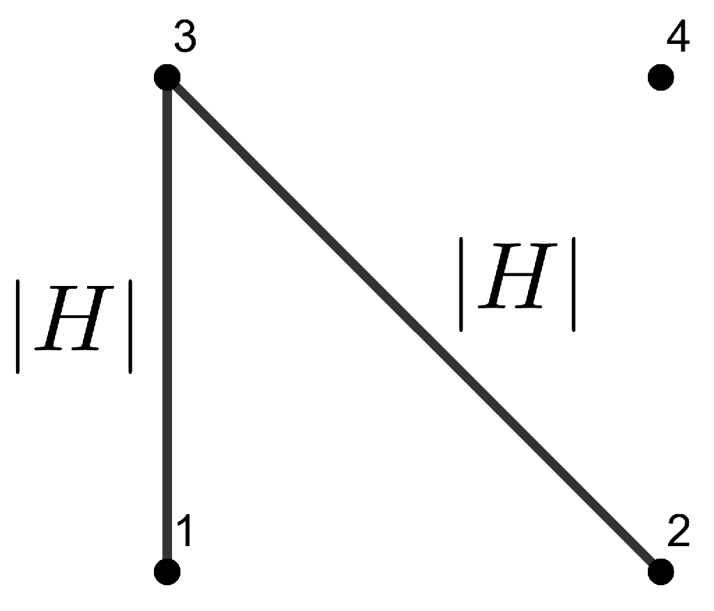
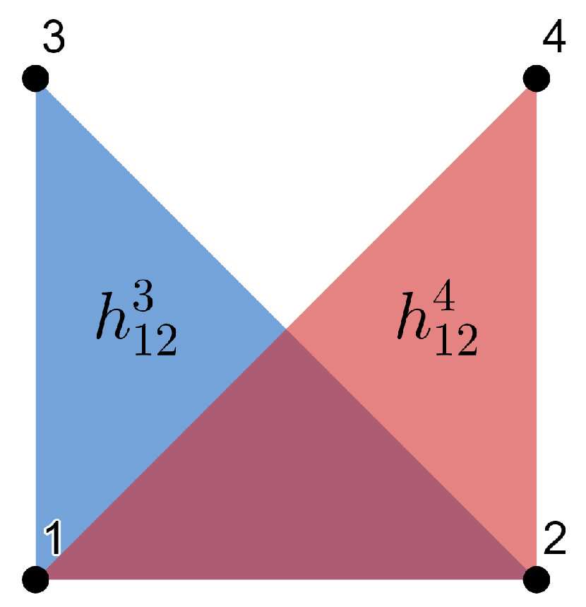
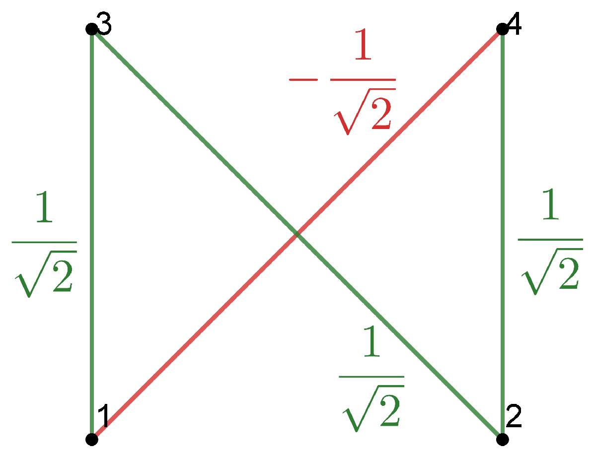
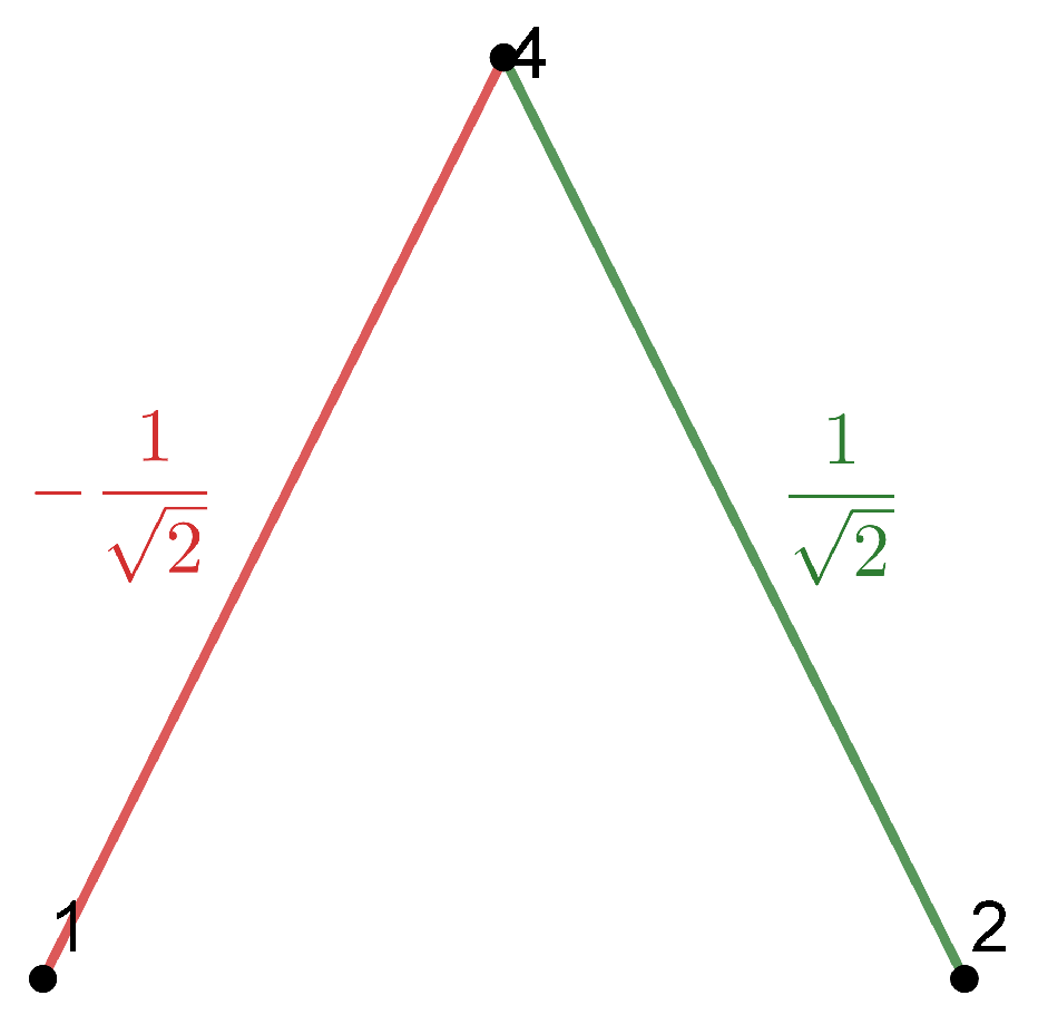
Example 1.

Consider a local orthonormal frame $\mathcal{B}=\{X_1,X_2,X_3,X_4\}$, such that $X_1,X_2$ are tangent to M and $X_3,X_4$ are normal to M. Then we can write the SFF as

$$\begin{array}{cc}\hfill & h(X_1,X_1)=h_{11}^3{X}_3+h_{11}^4{X}_4,\hfill \\ \hfill & h(X_1,X_2)=h_{12}^3{X}_3+h_{12}^4{X}_4,\hfill \\ \hfill & h(X_2,X_2)=h_{22}^3{X}_3+h_{22}^4{X}_4,\hfill \end{array}$$

and we obtain the combinatorial visualization shown in Figure 1.

Example 2.

Suppose that M is a totally umbilical surface with a non-zero mean curvature H. Then, we can fix the local orthonormal frame

$$\mathcal{B}=\{X_1,X_2,X_3={\displaystyle \frac{H}{\left|H\right|}},X_4\},$$

such that $X_1,X_2$ are tangent to M and $X_4$ is normal to the other fields. Then, the SFF results in

$$\begin{array}{cc}\hfill & h(X_1,X_1)=g(X_1,X_1)H=H=\left|H\right|X_3,\hfill \\ \hfill & h(X_1,X_2)=g(X_1,X_2)H=0,\hfill \\ \hfill & h(X_2,X_2)=g(X_2,X_2)H=H=\left|H\right|X_3,\hfill \end{array}$$

and we obtain the combinatorial visualization shown in Figure 2.

Example 3.

As above, suppose that M is a totally umbilical surface with a non-zero mean curvature H and consider the local orthonormal frame

$${\mathcal{B}}^{\prime }=\{Y_1=X_1,Y_2=X_2,Y_3=\frac{\sqrt{2}}{2}(X_3+X_4),Y_4=\frac{\sqrt{2}}{2}(X_3-X_4)\}.$$

Then, we obtain the representation drawn in Figure 3 (we use a color code for edges and triangles of the same weight).

Remark 1.

Examples 2 and 3 show that the representation depends on the chosen local orthonormal frames.

However, this representation allows us to consider the inverse procedure to obtain information concerning the submanifold.

Example 4.

Let M again be a surface immersed in a 4-dimensional Riemannian manifold $(\tilde{M},g)$ with a local orthonormal frame $\mathcal{B}=\{X_1,X_2,X_3,X_4\}$ whose representation can be visualized in Figure 4.

In a simple view, we note the absence of edges, which implies

$$h(X_i,X_i)=h_{ii}^3{X}_3+h_{ii}^4{X}_4=0\mathrm{for}i=1,2,$$

thus, the mean curvature vector field vanishes, and M is a minimal submanifold.

4. General Results

In this section we are going to present some results to point out the utility of this new representation on a general Riemannian manifold.

Proposition 1.

Let M be a hypersurface isometrically immersed in a $(m+1)$-dimensional Riemannian manifold $(\tilde{M},g)$. Then, there exists a local frame field of tangent vector fields to $\tilde{M}$ whose representation is that of Figure 5, where ${\lambda }_1,\cdots ,{\lambda }_m$ denote the eigenvalues of the shape operator $A_{X_{m+1}}$.

Proof. 

Let $\mathcal{B}=\{X_1,\cdots ,X_{m+1}\}$ be a local frame field where $X_1,\cdots ,X_m$ are tangent to M and $X_{m+1}$ is normal to M. One of the properties of the shape operator $A_{X_{m+1}}$ is that its induced matrix is symmetric. Therefore, by the spectral theorem of symmetric matrices, we know that there exists a local orthonormal frame field $\{X_1^{\prime },\cdots ,X_m^{\prime }\}$ of eigenvectors of $A_{X_{m+1}}$, whose eigenvalues are ${\lambda }_1,\cdots ,{\lambda }_m$, respectively. Then, we obtain the diagonal matrix

$$A_{X_{m+1}}=\left(\begin{array}{cccc}{\lambda }_1& & & \\ & {\lambda }_2& & \\ & & \ddots & \\ & & & {\lambda }_m\end{array}\right).$$

Therefore, with respect to the local frame field ${\mathcal{B}}^{\prime }=\{X_1^{\prime },\cdots ,X_m^{\prime },X_{m+1}\}$, we obtain

$$h_{ij}^{m+1}=g(h(X_i^{\prime },X_j^{\prime }),X_{m+1})=g(A_{X_{m+1}}{X}_i^{\prime },X_j^{\prime })=g({\lambda }_i{X}_i^{\prime },X_j^{\prime })={\delta }_{ij}{\lambda }_i.$$

We conclude that $h(X_i^{\prime },X_j^{\prime })={\delta }_{ij}{X}_{m+1}$, and the representation is that of Figure 5. □

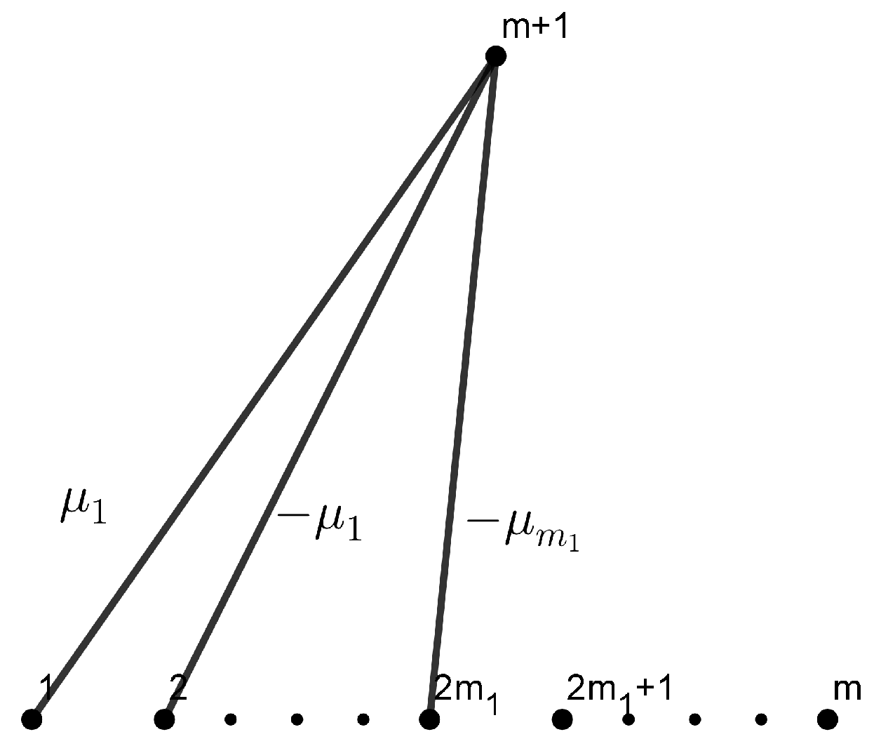
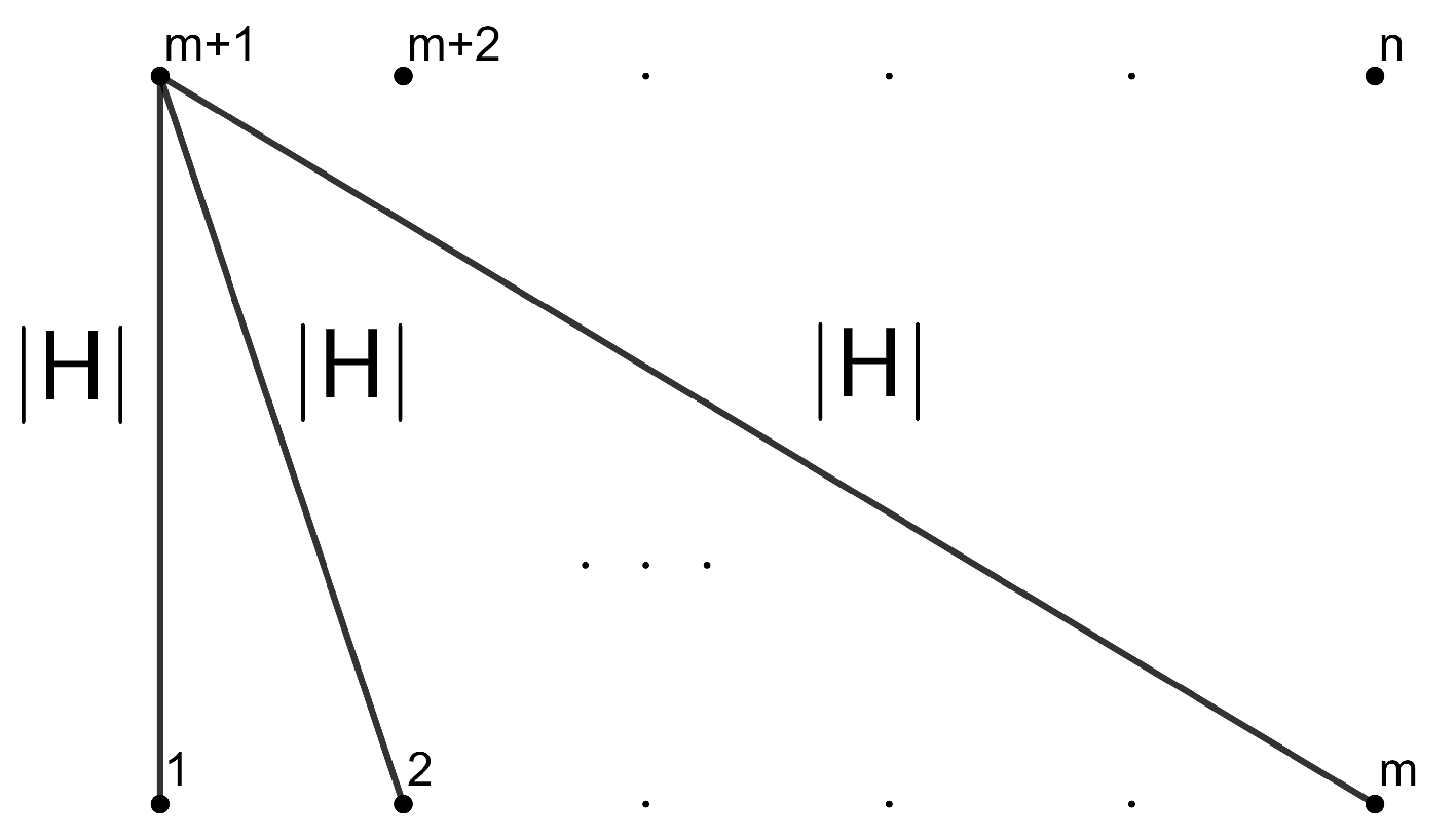
Corollary 1.

A hypersurface M isometrically immersed in a $(m+1)$-dimensional Riemannian manifold $(\tilde{M},g)$ is an austere submanifold if and only if there exists an orthonormal frame field $\{X_1,\cdots ,X_m,X_{m+1}\}$ of tangent vector fields to $\tilde{M}$ such that $X_{m+1}$ is normal to M and whose representation is Figure 6, where ${\mu }_1,-{\mu }_1,\cdots ,{\mu }_{m_1},-{\mu }_{m_1}$ are the non-zero eigenvalues of the shape operator $A_{X_{m+1}}$.

Theorem 1.

The representation of a totally umbilical submanifold with respect to any orthonormal frame field has no triangles.

Proof. 

Let M be a m-dimensional totally umbilical submanifold isometrically immersed in a n-dimensional Riemannian manifold $(\tilde{M},g)$, with H being the mean curvature vector. Consider an orthonormal frame field of the tangent vector field to $\tilde{M}$, $\mathcal{B}=\{X_1,\cdots ,X_n\}$, such that the first m vector fields are tangent to M. Then, it is clear that:

$$h(X_i,X_j)=g(X_i,X_j)H={\delta }_{ij}H,\mathrm{for}\mathrm{any}i,j\in \{1,\cdots ,m\}.$$

(1)

In particular, if $i\ne j$, then $h(X_i,X_j)=0$ so $h_{ij}^k=0$ for any $k\in \{m+1,\cdots ,n\}$. Consequently, the representation has no triangles. □

Theorem 2.

A (non-minimal) submanifold M isometrically immersed in a Riemannian manifold $(\tilde{M},g)$ is totally umbilical if and only if there exists a local orthonormal frame of tangent vector fields to $\tilde{M}$, whose representation is shown in Figure 7.

Proof. 

Firstly, if the submanifold is totally umbilical, consider an orthonormal frame field of the tangent vector field to $\tilde{M}$, $\mathcal{B}=\{X_1,\cdots ,X_n\}$ such that the first m vector fields are tangent to M and ${\displaystyle X_{m+1}=\frac{H}{\left|H\right|}}$.

Then, from (1), we easily obtain:

$$\begin{array}{cc}\hfill h_{ii}^1& =\left|H\right|,i=1,\cdots ,m,\hfill \\ \hfill h_{ii}^k& =0,i=1,\cdots ,m,k=m+2,\cdots ,n,\hfill \\ \hfill h_{ij}^k& =0,i,j=1,\cdots ,m,i\ne j,k=m+1,\cdots ,n.\hfill \end{array}$$

(2)

Conversely, suppose that there exists a local orthonormal frame field of the tangent vector field to $\tilde{M}$, $\mathcal{B}=\{X_1,\cdots ,X_n\}$ such that the first m vector fields are tangent to M and whose representation is given in Figure 7.

Then, for such a representation, we get:

$$\begin{array}{cc}\hfill H& =\frac{1}{m}\sum _{i=1}^{m}h(X_i,X_i)=\frac{1}{m}\sum _{i=1}^m\sum _{k=m+1}^n{h}_{ii}^k{X}_k\hfill \\ \hfill & =\frac{1}{m}\sum _{i=1}^m{h}_{ii}^1{X}_{m+1}=\left|H\right|X_{m+1}.\hfill \end{array}$$

Consequently, ${\displaystyle X_{m+1}=\frac{H}{\left|H\right|}}$. Then, from (2) and since $\mathcal{B}$ is the local orthonormal frame field:

$$\begin{array}{cc}\hfill \mathrm{If}i\ne j,& h(X_i,X_j)=0=g(X_i,X_j)H\hfill \\ \hfill \mathrm{If}i=j,& h(X_i,X_i)=h_{ii}^1{X}_{m+1}=H=g(X_i,X_i)H.\hfill \end{array}$$

Consequently, by using the linearity of fundamental forms, the submanifold is totally umbilical. □

Proposition 2.

A submanifold M is minimal if and only if there exists a frame field whose representation satisfies that the weights of the incident edges of each vertex associated to the normal fields of M add up to zero.

Proof. 

Let us suppose that M is minimal. Then, we have:

$${\displaystyle 0=\frac{1}{m}\sum _{i=1}^{m}h(X_i,X_i)=\frac{1}{m}\sum _{k=m+1}^n(\sum _{i=1}^m{h}_{ii}^k)X_k.}$$

Therefore, ${\displaystyle \sum _{=1}^m{h}_{ii}^k=0}$ for every $k\in \{m+1,\cdots ,n\}$. Thus, we conclude the proof of the proposition. □

Corollary 2.

If, for a local frame field, the representation only has triangles, the represented submanifold is minimal.

5. Lagrangian Submanifolds of Kaehler Manifolds

In this section, let $(\tilde{M},J,g)$ be a $2m$-dimensional Kaehler manifold and consider a Lagrangian submanifold M isometrically immersed in $\tilde{M}$. Let $\mathcal{B}$ be an adapted Lagrangian frame field [4],

$$\mathcal{B}=\{X_1,\cdots ,X_m,X_{1^{\prime }}=J{X}_1,\cdots ,X_{m^{\prime }}=J{X}_m\}$$

where $\{X_1,\cdots ,X_m\}$ is a local frame field for tangent vector fields to M. We say that the representation obtained by using this adapted Lagrangian frame field is a Lagrangian representation of M.

Lemma 1.

Every Lagrangian representation of a submanifold M of a Kaehler manifold $\tilde{M}$ satisfies that

$$h_{ij}^{k^{\prime }}=h_{ik}^{j^{\prime }}=h_{jk}^{i^{\prime }},$$

(3)

for any $i,j,k\in \{1,\cdots ,m\}$.

Proof. 

Given $h_{ij}^{k^{\prime }}$, we have $h_{ij}^{k^{\prime }}=h_{ik}^{j^{\prime }}$ due to the properties of the Kaehler ambient manifold and the anti-symmetry of the almost complex structure J. By using the symmetry of the SFF, we obtain

$$h_{ij}^{k^{\prime }}=h_{ik}^{j^{\prime }}=h_{ki}^{j^{\prime }}=h_{jk}^{i^{\prime }},$$

which implies (3). □

Corollary 3.

Let M be a Lagrangian submanifold of a Kaehler manifold. If a Lagrangian representation of M has no triangles, then $h_{ij}^{k^{\prime }}$ is non-zero if and only if $i=h=k$.

Proof. 

Let us suppose that there exists an edge $h_{ii}^{k^{\prime }}\ne 0$ with $i\ne k$. Therefore, from Lemma 1, $h_{ii}^{k^{\prime }}=h_{ik}^{i^{\prime }}\ne 0$, which is a contradiction because the representation has no triangles.

The other implication is analogous. □

Theorem 3.

Let M be a m-dimensional ($m>1$) Lagrangian and totally umbilical submanifold of a Kaehler manifold. Then, M is minimal.

Proof. 

Suppose that M is not minimal; that is, that the mean curvature vector H is not zero. Let

$${\displaystyle \mathcal{B}=\{X_1=-J{X}_{1^{\prime }},X_2,\cdots ,X_m,X_{1^{\prime }}=\frac{H}{\left|H\right|},X_{2^{\prime }}=J{X}_2,\cdots ,X_{m^{\prime }}=J{X}_m\}}$$

be an adapted Lagrangian frame field of M. We now have:

$$h(X_2,X_2)=g(X_2,X_2)H=1·\left|H\right|·X_{1^{\prime }}=\left|H\right|·X_{1^{\prime }}.$$

Therefore, $h_{22}^{1^{\prime }}=\left|H\right|$, and due to Lemma 1, $\left|H\right|=h_{22}^{1^{\prime }}=h_{12}^{2^{\prime }}$. However, we know that $h_{12}^{2^{\prime }}=g(h(X_1,X_2),X_{2^{\prime }})=g(g(X_1,X_2)H,X_{2^{\prime }})=g\left(\right|H|X_{1^{\prime }},X_{2^{\prime }})=0\ne H$, which is a contradiction. We conclude that $M^m$ is a minimal submanifold. □

Corollary 4.

Any m-dimensional ($m>1$) Lagrangian and totally umbilical submanifold of a Kaehler manifold is totally geodesic.

6. Example: The Clifford Torus

The Clifford torus is a special type of torus with ${\displaystyle \frac{1}{\sqrt{2}}}{S}^1\times {\displaystyle \frac{1}{\sqrt{2}}}{S}^1$ inside ${\mathbb{R}}^2\times {\mathbb{R}}^2={\mathbb{R}}^4$. It actually lies in the unit sphere $S^3$ because each point has the same distance to the origin. Then, it is well known that the Clifford torus with the Euclidean metric is an austere submanifold of $S^3\left(1\right)$ [8]. We are going to reach this conclusion by using this new representation.

Consider $f:{\mathbb{R}}^2\to {\mathbb{R}}^4$, given by:

$$f(\theta ,\varphi )={\displaystyle \frac{1}{\sqrt{2}}}(cos\theta ,sin\theta ,cos\phi ,sin\phi ),(\theta ,\phi )\in {\mathbb{R}}^2.$$

The mapping f is an immersion of ${\mathbb{R}}^2$ into the unit sphere $S^3\left(1\right)\subset {\mathbb{R}}^4$, where the image $f\left({\mathbb{R}}^2\right)$ is the flat torus. The vector fields

$$\begin{array}{cc}\hfill & e_1=(-sin\theta ,cos\theta ,0,0)\hfill \\ \hfill & e_2=(0,0,-sin\phi ,cos\phi )\hfill \end{array}$$

form an orthonormal basis of the tangent space $T_{f(\theta ,\varphi )}Imf$, and the normal vectors

$$\begin{array}{cc}\hfill & e_3={\displaystyle \frac{1}{\sqrt{2}}}(cos\theta ,sin\theta ,cos\phi ,sin\phi )\hfill \\ \hfill & e_4={\displaystyle \frac{1}{\sqrt{2}}}(-cos\theta ,-sin\theta ,cos\phi ,sin\phi )\hfill \end{array}$$

form an orthonormal basis of the normal space. The matrices $A_{e_3}$ and $A_{e_4}$ with respect to the basis $\{e_1,e_2\}$ are:

$$A_{e_3}=\left(\begin{array}{cc}-\frac{1}{\sqrt{2}}& 0\\ 0& -\frac{1}{\sqrt{2}}\end{array}\right),A_{e_4}=\left(\begin{array}{cc}\frac{1}{\sqrt{2}}& 0\\ 0& -\frac{1}{\sqrt{2}}\end{array}\right).$$

Therefore, the second fundamental form is given by:

$$\begin{array}{cc}\hfill & h(e_1,e_1)=-{\displaystyle \frac{1}{\sqrt{2}}}{e}_3+{\displaystyle \frac{1}{\sqrt{2}}}{e}_4,\hfill \\ \hfill & h(e_2,e_2)=-{\displaystyle \frac{1}{\sqrt{2}}}{e}_3-{\displaystyle \frac{1}{\sqrt{2}}}{e}_4,\hfill \\ \hfill & h(e_1,e_2)=0.\hfill \end{array}$$

In this context, the submanifold representation is presented in Figure 8 and Figure 9 (in the representation, we also include a color code to clarify the edges and triangles of the same weight).

We observe that the Figure 9 is an austere submanifold of $S^3$ in virtue of Corollary 1.