A Bivariate Optimal Random Replacement Model for the Warranted Product with Job Cycles

Abstract

A monitoring system (MS) has been used to monitor products’ job cycles. It is indicated that by incorporating the job cycle into the product’s life cycle, warrantors can devise novel warranty models and consumers can define and model random maintenances sustaining the reliability of the product through warranty. In this study, by incorporating limited job cycles and a refund into the traditional free repair warranty, a two-dimensional free repair warranty with a refund (2DFRW-R) is devised for guaranteeing the product reliability to consumers. Under the condition that 2DFRW-R is planned to guarantee product reliability, a bivariate random periodic replacement (BRPR) (i.e., a random periodic replacement where the accomplishment of the Nth job cycle and the replacement time T are designed as replacement limits) is modeled to sustain the post-warranty reliability from the point of view of the consumer. From the point of view of the warrantor, the warranty cost related to 2DFRW-R is derived, and the characteristics of 2DFRW-R are explored. From the point of view of consumers, the expected cost rate related to BRPR is constructed, and the existence and uniqueness of the optimal BRPR are summarized as well. By discussing parameters, several special cases are derived. The characteristics of the proposed models are analyzed in numerical examples.

1. Introduction

The core competitiveness of products depends on product price, product functionality, after-sales service, etc. Among them, after-sales service is not only a powerful guarantee of consumer rights and interests but also a key factor in improving brand image. As the main term of after-sales service, the warranty policy is an important factor that affects product sales and brand image improvement.

Due to the above important values, warranties have been studied extensively from the point of view of warrantors (or manufacturers). According to the technologies of reliability modeling, warranties are divided into the lifetime-based warranty, the on-condition warranty, and the performance-based warranty. Usually, the lifetime-based warranty is designed based on a distribution function of the product’s lifetime. This kind of warranty includes two-dimensional warranties in [1,2,3,4,5], one-dimensional warranties in [6,7,8,9,10,11,12,13], and three-dimensional warranties in [14], wherein the product’s lifetime is subject to a distribution function. The on-condition warranty is designed based on a stochastic degradation process. For example, Ref. [15] designed an on-condition-based renewable free replacement warranty for the product subject to an inverse Gaussian process; Ref. [16] devised an on-condition warranty by assuming that product deterioration is modeled by a Gamma process; Ref. [17] designed an optimal on-condition warranty for the product subject to a Wiener process. The performance-based warranty is designed based on a mixture of stochastic degradation processes and distribution functions. For example, Ref. [18] modeled a performance-based warranty by combining a stochastic degradation process and a distribution function.

Although each of the above types of warranty can guarantee product reliability, this kind of guarantee is limited to the warranty period rather than the whole life cycle of the product. Therefore, consumers must focus on how to guarantee post-warranty reliability. In view of this, a variety of maintenance models were proposed from the point of view of consumers to sustain the post-warranty reliability and lower maintenance costs after the warranty expiration. The related maintenance models are classified as either the on-condition maintenance model or the lifetime-based maintenance model. Previously, Reference [15] proposed the on-condition maintenance model to sustain the post-warranty reliability, wherein an inverse Gaussian process characterizes the product’s degradation. References [19,20,21] designed and optimized the lifetime-based maintenance models sustaining the post-warranty reliability by letting the product’s lifetime obey a distribution function.

From the viewpoint of an engineering practice, the development and application of the monitoring system (MS) makes it possible to diagnose the health condition of products. In addition, MS is able to monitor the job cycle of the product that works for tasks. For example, in China, sharing bikes (SB) are helping the construction of green and low-carbon cities. By means of MS, SB providers (or users) can monitor the real-time usage of each SB. From reliability theory, the job time that can be estimated by job cycles significantly affects the deterioration of the product working for tasks. Considering this fact [22,23,24,25] integrated the working cycle (i.e., job cycle) into maintenance theory and studied some random maintenance models that are used for ensuring the product reliability.

Similarly, by designing the limited job cycles a warranty constraint, some novel warranty models can be devised for ensuring product reliability from the point of view of the warrantor; by designing the limited job cycles a replacement limit, some random maintenance models to sustain the post-warranty reliability are investigated from the point of view of the consumer. By designing the limited job cycles a warranty constraint [26], earlier proposed the warrantor’s two-dimensional free repair warranty models so as to ensure the product reliability, alike earlier investigated consumers’ periodic replacement models, which are used for sustaining the post-warranty reliability.

The two-dimensional free repair warranty first (2DFRWF) in [26] satisfies that (1) minimal repair is used for removing all product failures before the accomplishment of the $m\mathrm{th}$ job cycle or before the warranty period w, whichever comes first; (2) warrantors bear the costs of removing all failures. This warranty classifies consumers into two populations. The first population is people whose warranty expiry occurs before the warranty period $w$ at the accomplishment of the $m\mathrm{th}$ job cycle. The second population is people whose warranty expires before the accomplishment of the $m\mathrm{th}$ job cycle at the warranty period $w$. The warranty service period (i.e., a sum of $m$ job cycles) of the former is lower than that (i.e., the length $w$ of the warranty period) of the latter. The occurrence of this case may make the former perceive that they are not treated as equal as the latter. If this perception appears in the first population, then some consumers from the first population will complain to the consumers’ union (CU), and thus the brand image of warrantors is inevitably damaged. If the refund in [27,28] is used as compensation for consumers from the first population, then the complaint no longer exists and the brand image is not damaged. By reviewing the literature on warranties, however, it is found that the two-dimensional free repair warranty considering a refund has not been studied to eliminate the consumer’s complaint and ensure the brand image.

In addition, random periodic replacement first (RPRF) to sustain the post-warranty reliability in [26] requires that consumers replace the product through warranty at the replacement time $T$ or the accomplishment of a job cycle, which comes first. Under these requirements, the post-warranty period produced by the replacement at the accomplishment of a job cycle is obviously lower than the post-warranty period produced by the replacement at $T$. Once the former type of replacement occurs, most of the remaining life for the product through warranty is easily wasted rather than serving consumers. If the replacement at the accomplishment of a job cycle is expanded to the replacement at the accomplishment of the $N\mathrm{th}$ job cycle, most of the remaining life for the product through warranty unquestionably serves consumers as much as possible, rather than wasting largely. However, random periodic replacement policies that incorporate the replacement at the accomplishment of the $N\mathrm{th}$ job cycle have not been studied to guarantee the post-warranty reliability.

In this study, by integrating a refund into the first type of warranty (i.e., 2DFRWF) in [26], a warrantor’s warranty model is devised to eliminate consumer complaints and ensure the brand image. The devised warranty is a two-dimensional free repair warranty with a refund (2DFRW-R) requiring the following: ① if the $m\mathrm{th}$ job cycle is accomplished before the warranty period $w$, then the warrantor will provide a refund for making the consumers perceive themselves to be treated fairly, while the warranty service expires at the accomplishment of the $m\mathrm{th}$ job cycle; ② if the warranty period $w$ will be reached before the $m\mathrm{th}$ job cycle is accomplished, then the consumer no longer obtains a refund from the warrantor and while the warranty service expires at the warranty period $w$. In addition, for largely using the remaining life of the product through warranty, we incorporate $N$ job cycles into periodic replacement and investigate a bivariate random periodic replacement (BRPR) requiring that the product through 2DFRW-R be replaced when the $N\mathrm{th}$ job cycle is accomplished or when the replacement time $T$ is reached, whichever comes earlier. We construct the expected cost rate of BRPR, analyze the existence and uniqueness of the optimal BRPR, and explore the characteristics of the proposed models in numerical examples.

The study’s contributions are highlighted as having two key aspects: (1) by integrating both $m$ job cycles and a refund into classic free repair warranty model, a warrantor’s warranty model with fairness characteristics is devised to guarantee the product reliability; (2) a consumer’s BRPR model is studied for sustaining the post-warranty reliability and largely using the remaining life of the product through warranty.

The structure of the present study is listed as follows. 2DFRW-R is defined and the corresponding warranty cost is modeled in Section 2. Section 3, from the point of view of the consumer, presents the definition of BRPR and models the cost rate. In Section 4, the characteristics of 2DFRW-R and BRPR are analyzed in numerical examples. The final conclusion is offered in Section 5.

2. Warrantors’ Warranty Model

Assume that the product works for tasks at job cycles and that the job cycle $Y_i$ of the $i\mathrm{th}$ ($i=1,2,\dots$) task is independent and obeys the identical distribution function $G(y)=\mathrm{Pr}\{Y_i<y\}$ that has no memory. The product’s first failure time $X$ obeys the distribution function $F(x)=\mathrm{Pr}\{X<x\}$, wherein $r(u)$ is a failure rate function. Furthermore, the time to repair and replacement is assumed to be negligible.

2.1. Warranty Model Definition

Let $w$ and $m$ ($0<m<\infty$) be the warranty period and the number of job cycles, respectively; denote $S_m$ by the product’s job time when the $m\mathrm{th}$ job cycle is accomplished, where $S_m={\displaystyle \sum _{i=1}^m{Y}_i}$; then, a warranty is described as follows.

• The warranty expires when the $m\mathrm{th}$ job cycle is accomplished or when the warranty period $w$ is reached, whichever comes earlier.
• The warrantor uses minimal repair to eliminate all product failures that occur before the accomplishment of the $m\mathrm{th}$ job cycle or before the warranty period $w$, whichever comes earlier.
• If the warranty expires before the warranty period $w$ at the accomplishment of the $m\mathrm{th}$ job cycle, the warrantor will provide the consumer with a refund depending on the job time, which is used as a type of maintenance fund in the time interval $(S_m,w]$.
• The warrantor absorbs each repair cost, which is the unit cost of eliminating each failure.

Please note that ① if the refund in this warranty is removed, this warranty is the same as the first type of the two-dimensional free repair warranty (2DFRW) in [26], wherein ‘whichever occurs first’ is considered. In view of this, such a warranty is called a two-dimensional free repair warranty with a refund (2DFRW-R); ② the case where 2DFRW-R expires is classified into two kinds. The first kind is that 2DFRW-R expires before the warranty period $w$ at the accomplishment of the $m\mathrm{th}$ job cycle, and the second kind is that 2DFRW-R expires before the accomplishment of the $m\mathrm{th}$ job cycle at the warranty period $w$. Correspondingly, consumers can also be divided into two populations. The first population is that people whose 2DFRW-R expires before the warranty period $w$ at the accomplishment of the $m\mathrm{th}$ job cycle. The second population includes people whose 2DFRW-R expires before the accomplishment of the $m\mathrm{th}$ job cycle at the warranty period $w$; ③ the warranty service period of the first population is $S_m$, where $S_m<w$, and the warranty service period of the second population equates to $w$, where $w<S_m$. Obviously, the warranty service period $S_m$ of the first population is shorter than the warranty service period $w$ of the second population. Because this fact can make the first population perceive that they are not treated as equal to the second population, it is unavoidable to have complaints from the first population, which can damage the brand image. Therefore, refunds should be provided to compensate the first population, eliminate the first population’s complaints, and ensure a good brand image.

For convenience, hereinafter, we will refer to the case in which 2DFRW-R expires before the warranty period $w$ at the accomplishment of the $m\mathrm{th}$ job cycle as “2DFRW-R expires at the accomplishment of the $m\mathrm{th}$ job cycle”, and will refer to the case in which 2DFRW-R expires before the accomplishment of the $m\mathrm{th}$ job cycle at the warranty period $w$ as “2DFRW-R expires at the warranty period $w$”.

2.2. Warranty Cost Model

From [29], the distribution function $G^{(m)}(s)$ of the job time $S_m$ (i.e., a random variable) is a Stieltjes convolution $G^{(m)}(s)=\mathrm{Pr}\left\{S_m<s\right\}={\displaystyle {\int }_0^s{G}^{(m-1)}(s-u)\mathrm{d}G(u)}$, and the reliability function ${\overline{G}}^{(m)}(s)$ of the job time $S_m$ is ${\overline{G}}^{(m)}(s)=\mathrm{Pr}\left\{S_m>s\right\}=1-{\displaystyle {\int }_0^s{G}^{(m-1)}(s-u)\mathrm{d}G(u)}$. When 2DFRW-R expiration occurs at the accomplishment of the $m\mathrm{th}$ job cycle, the warranty service period equates to $S_m$ with the distribution function $H(s)$:

$$H(s)=\mathrm{Pr}\left\{S_m<s|S_m<w\right\}=\mathrm{Pr}\left\{S_m<s\right\}/\mathrm{Pr}\left\{S_m<w\right\}=G^{(m)}(s)/G^{(m)}(w)$$

(1)

where $0<s<w$.

For 2DFRW-R, minimal repair can remove all product failures. Let $c_m$ be the unit repair cost. Therefore, when 2DFRW-R expires at the accomplishment of the $m\mathrm{th}$ job cycle, the total repair cost $C_{S_m}(S_m)$ of the warrantor is given by

$$C_{S_m}(S_m)=c_m{\displaystyle {\int }_0^{S_m}r(u)\mathrm{d}u}$$

(2)

Since the distribution function of $S_m$ is $H(s)$ in (1), the expected value $W{C}_{S_m}$ of the total repair cost $C_{S_m}(S_m)$ is represented by

$$W{C}_{S_m}={\displaystyle {\int }_0^w{C}_{S_m}(s)\mathrm{d}H(s)}=\frac{c_m{\displaystyle {\int }_0^w\left({\displaystyle {\int }_0^{s}r(u)\mathrm{d}u}\right)\mathrm{d}{\overline{G}}^{(m)}(s)}}{{\overline{G}}^{(m)}(w)}$$

(3)

Similar to (2), when 2DFRW-R expires at the warranty period $w$, the total repair cost $W{C}_w$ of the warrantor is represented by

$$W{C}_w=c_m{\displaystyle {\int }_0^{w}r(u)\mathrm{d}u}$$

(4)

According to the definition of 2DFRW-R, the probability that 2DFRW-R expires at the accomplishment of the $m\mathrm{th}$ job cycle can be given by $G^{(m)}(w)$; alike, the probability that 2DFRW-R expiry occurs at the warranty period $w$ can be given by ${\overline{G}}^{(m)}(w)$. Therefore, the total repair cost $W{C}_m$ of 2DFRW-R is expressed as

$$\begin{array}{ll}W{C}_m& =G^{(m)}(w)\cdot W{C}_{S_m}+{\overline{G}}^{(m)}(w)\cdot W{C}_w\\ & =c_m\left({\displaystyle {\int }_0^w\left({\displaystyle {\int }_0^{s}r(u)\mathrm{d}u}\right)\mathrm{d}{G}^{(m)}(s)}+{\overline{G}}^{(m)}(w){\displaystyle {\int }_0^{w}r(u)\mathrm{d}u}\right)\\ & =c_m{\displaystyle {\int }_0^w{\overline{G}}^{(m)}(s)r(s)\mathrm{d}s}\end{array}$$

(5)

When 2DFRW-R expires at the accomplishment of the $m\mathrm{th}$ job cycle, the warrantor provides the consumer a refund that is used as a special maintenance fund in the time interval $(S_m,w]$. Let the decreased function $R(S_m)$ be a refund at the job time $S_m$; then, we model the refund $R(S_m)$ as

$$R(S_m)=\{\begin{array}{ll}a{c}_R{\left(1-\frac{\kappa S_m}{w}\right)}^b,& for S_m<w\\ 0,& for S_m\ge w \end{array}$$

(6)

where $a>0$, $b>0$, $c_R>0$ and $0<\kappa \le 1$.

If and only if 2DFRW-R expires at the accomplishment of the $m\mathrm{th}$ job cycle, does the warrantor provide the consumer with a corresponding refund $R(S_m)$. As mentioned above, the probability that 2DFRW-R expires at the accomplishment of the $m\mathrm{th}$ job cycle is $G^{(m)}(w)$; in addition, $S_m$ in the refund $R(S_m)$ obeys the distribution function $H(s)$ in (1). Therefore, the expected value $R$ of the refund $R(S_m)$ can be calculated as

$$R=G^{(m)}(w)\cdot E[R(S_m)]=G^{(m)}(w)\cdot {\displaystyle {\int }_0^{w}R(s)\mathrm{d}H(s)} = a{c}_R{\displaystyle {\int }_0^w{\left(w-\kappa s\right)}^b}\mathrm{d}{G}^{(m)}(s)/w^b$$

(7)

According to the definition of 2DFRW-R, the warranty cost of 2DFRW-R includes the total repair cost $W{C}_m$ and the expectation $R$ of the refund $R(S_m)$. Thus, the warranty cost $WC$ of 2DFRW-R is given by

$$WC=W{C}_m+R=c_m{\displaystyle {\int }_0^w{\overline{G}}^{(m)}(s)r(s)\mathrm{d}s}+ a{c}_R{\displaystyle {\int }_0^w{\left(w-\kappa s\right)}^b}\mathrm{d}{G}^{(m)}(s)/w^b$$

(8)

Obviously, $\underset{m\to \infty }{\lim }{\overline{G}}^{(m)}(s)=1$ and $\underset{m\to \infty }{\lim }{G}^{(m)}(s)=0$. It is indicated that if $m\to \infty$, the warranty limit $m$ is invalid, and thus the refund is removed. Therefore, the warranty cost model in (8) is reduced to $\underset{m\to \infty }{\lim }WC=c_m{\displaystyle {\int }_0^{w}r(s)\mathrm{d}s}$, which represents the warranty cost of the free repair warranty (FRW) in [30].

In addition, the warranty cost $WC$ of 2DFRW-R is greater than the warranty cost (which has been modeled as $c_m{\displaystyle {\int }_0^w{\overline{G}}^{(m)}(s)r(s)\mathrm{d}s}$) of 2DFRWF in [26], i.e.,

$$c_m{\displaystyle {\int }_0^w{\overline{G}}^{(m)}(s)r(s)\mathrm{d}s}+ a{c}_R{\displaystyle {\int }_0^w{\left(w-\kappa s\right)}^b}\mathrm{d}{G}^{(m)}(s)/w^b>c_m{\displaystyle {\int }_0^w{\overline{G}}^{(m)}(s)r(s)\mathrm{d}s}$$

Such an inequality means that ① from the point of view of the warrantor, 2DFRW-R can eliminate the complaints from the first population and ensure the brand image, but its warranty cost cannot be reduced compared with 2DFRWF; ② between 2DFRWF in [26] and 2DFRW-R, consumers have a preference for 2DFRW-R because it means that they possibly obtain a refund from the warrantor.

3. Bivariate Random Periodic Replacement Model of Consumers

In the case that RPRF in [26] is used for sustaining the post-warranty reliability, the product with higher job frequency and shorter job cycles is very easily replaced before the replacement time $T$ at the accomplishment of a job cycle. The occurrence of this case wastes the remaining life of the product through the warranty rather than largely serving the consumers. If the replacement before the replacement time $T$ at the accomplishment of a job cycle is expanded to a replacement before the replacement time $T$ at the accomplishment of the $N\mathrm{th}$ job cycle, the remaining life of the product through warranty can serve the consumer as much as possible, rather than wasting largely.

In view of this, by expanding the accomplishment of a job cycle to the accomplishment of the $N\mathrm{th}$ ($N=1,2,\cdots$) job cycle, this section models a bivariate random periodic replacement (BRPR), which is used for sustaining the post-warranty reliability of the product that is warranted by 2DFRW-R and largely using the remaining life of the product through 2DFRW-R. Such a BRPR requires ① the product through 2DFRW-R is preventively replaced at the accomplishment of the $N\mathrm{th}$ job cycle or at the replacement time $T$, whichever comes earlier; ② the product through 2DFRW-R undergoes minimal repair at failure before replacement. When $N=1$, such a BRPR is reduced to a univariate replacement, which is represented as RPRF in [26].

To model BRPR conveniently, it is defined that the product’s life cycle is a span that begins from the accomplishment of a new product installation and ends the replacement occurrence at the cost of the consumer, which is similar to [19,20,21]. Clearly, this type of life cycle includes the warranty service period of 2DFRW-R and the post-warranty period of BRPR.

3.1. Total Cost during the Life Cycle

As mentioned above, it is assumed that the job cycle $Y_i$ is independent and obeys the identical distribution $G(y)$ that has no memory. Such an assumption shows that the task’s remaining accomplishment time and each job cycle during the post-warranty period are still independent and obey the identical distribution $G(y)$, which has no memory. When the product through 2DFRW-R is preventively replaced at the accomplishment of the $N\mathrm{th}$ job cycle, the job time during the post-warranty period is $S_N$, where $S_N={\displaystyle \sum _{i=1}^N{Y}_i}$. The respective probabilities that the product through 2DFRW-R is preventively replaced before the replacement time $T$ at the accomplishment of the $N\mathrm{th}$ job cycle or before the accomplishment of the $N\mathrm{th}$ job cycle at the replacement time $T$ are $G^{(N)}(T)=\mathrm{Pr}\{S_N<T\}={\displaystyle {\int }_0^T{G}^{(N-1)}(T-u)\mathrm{d}G(u)}$ and ${\overline{G}}^{(N)}(T)=\mathrm{Pr}\{T<S_N\}=1-{\displaystyle {\int }_0^T{G}^{(N-1)}(T-u)\mathrm{d}G(u)}$.

Denote $c_f$ by the unit failure cost of each failure occurrence. When 2DFRW-R expires at the accomplishment of the $m\mathrm{th}$ job cycle and when the product through 2DFRW-R is preventively replaced before the replacement time $T$ at the accomplishment of the $N\mathrm{th}$ job cycle, the total cost $C_m(S_N)$ of BRPR can be computed as

$$C_m(S_N)=(c_f+c_m){\displaystyle {\int }_0^{S_N}r(S_m+u)\mathrm{d}u}$$

(9)

where $S_N<T$; $c_f+c_m$ is the total cost resulting from each failure; and $r(S_m+u)$ is a failure rate function at $S_m$.

When 2DFRW-R expires at the accomplishment of the $m\mathrm{th}$ job cycle and when the product through 2DFRW-R is preventively replaced before the accomplishment of the $N\mathrm{th}$ job cycle at the replacement time $T$, the total cost $C_m(T)$ of BRPR is computed as

$$C_m(T)=(c_f+c_m){\displaystyle {\int }_0^{T}r(S_m+u)\mathrm{d}u}$$

(10)

Under the case where 2DFRW-R expires at the accomplishment of the $m\mathrm{th}$ job cycle, the total cost $C_{S_m}(N,T;S_m)$ of BRPR is derived as

$$\begin{array}{ll}{C}_{S_m}(N,T;S_m)& =G^{(N)}(T)\cdot {\displaystyle {\int }_0^T{C}_m(t)\mathrm{d}I(t)}+ {\overline{G}}^{(N)}(T)\cdot C_m(T)+c_P\\ & =(c_f+c_m){\displaystyle {\int }_0^T\left({\displaystyle {\int }_0^{t}r(S_m+u)\mathrm{d}u}\right)\mathrm{d}{G}^{(N)}(t)}+ {\overline{G}}^{(N)}(T)(c_f+c_m){\displaystyle {\int }_0^{T}r(S_m+u)\mathrm{d}u}+c_P\\ & =(c_f+c_m){\displaystyle {\int }_0^T{\overline{G}}^{(N)}(t)r(S_m+t)\mathrm{d}t}+c_P\end{array}$$

(11)

where the distribution function $I(t)$ of $S_N$ satisfies $I(t)=\mathrm{Pr}\left\{S_N<t|S_N<T\right\}=G^{(N)}(t)/G^{(N)}(T)$ ($0<t<T$); $c_P$ represents the unit replacement cost, where $c_P>c_R$.

When 2DFRW-R expires at the warranty period $w$ and when the product through 2DFRW-R is preventively replaced before the replacement time $T$ at the accomplishment of the $N\mathrm{th}$ job cycle, the total cost $C_w(S_N)$ of BRPR is computed as

$$C_w(S_N)=(c_f+c_m){\displaystyle {\int }_0^{S_N}r(w+u)\mathrm{d}u}$$

(12)

where $S_N<T$.

When 2DFRW-R expiry occurs at the warranty period $w$ and when the product through 2DFRW-R is preventively replaced before the accomplishment of the $N\mathrm{th}$ job cycle at the replacement time $T$, the total cost $C_w(S_N)$ of BRPR is computed as

$$C_w(T)=(c_f+c_m){\displaystyle {\int }_0^{T}r(w+u)\mathrm{d}u}$$

(13)

Under the case in which 2DFRW-R expiry occurs at the warranty period $w$, the total cost $C_w(N,T;w)$ of BRPR is derived as

$$\begin{array}{ll}{C}_w(N,T;w)& =G^{(N)}(T)\cdot {\displaystyle {\int }_0^T{C}_w(t)\mathrm{d}I(t)}+ {\overline{G}}^{(N)}(T)\cdot C_w(T)+c_P\\ & =(c_f+c_m){\displaystyle {\int }_0^T\left({\displaystyle {\int }_0^{t}r(w+u)\mathrm{d}u}\right)\mathrm{d}{G}^{(N)}(t)}+ {\overline{G}}^{(N)}(T)(c_f+c_m){\displaystyle {\int }_0^{T}r(w+u)\mathrm{d}u}+c_P\\ & =(c_f+c_m){\displaystyle {\int }_0^T{\overline{G}}^{(N)}(t)r(w+t)\mathrm{d}t}+c_P \end{array}$$

(14)

Under the case where 2DFRW-R warrants the product, the expected total cost $C_{pw}(N,T)$ of BRPR is calculated as

$$\begin{array}{ll}{C}_{pw}(N,T)& =G^{(m)}(w)\cdot {\displaystyle {\int }_0^w{C}_{S_m}(N,T;s)\mathrm{d}H(s)}+{\overline{G}}^{(m)}(w)\cdot C_w(N,T;w)\\ & =(c_f+c_m){\displaystyle {\int }_0^w\left({\displaystyle {\int }_0^T{\overline{G}}^{(N)}(t)r(s+t)\mathrm{d}t}\right)}\mathrm{d}{G}^{(m)}(s)+{\overline{G}}^{(m)}(w)(c_f+c_m){\displaystyle {\int }_0^T{\overline{G}}^{(N)}(t)r(w+t)\mathrm{d}t}+c_p\\ & = (c_f+c_m)\left({\displaystyle {\int }_0^w{\overline{G}}^{(m)}(s)\mathrm{d}\left({\displaystyle {\int }_0^T{\overline{G}}^{(N)}(t)r(s+t)\mathrm{d}t}\right)}+{\displaystyle {\int }_0^T{\overline{G}}^{(N)}(t)r(t)\mathrm{d}t}\right)+c_p\end{array}$$

(15)

As mentioned above, the life cycle is a sum of the warranty service period of 2DFRW-R and the post-warranty period of BRPR. This indicates that the total cost during the life cycle is composed of the total failure cost of 2DFRW-R, the expectation $R$ of the refund related to 2DFRW-R, and the expected total cost of BRPR. By replacing $c_m$ in $W{C}_m$ of (5) with $c_f$, the total failure cost $C_{fc}$ of 2DFRW-R is computed as $C_{fc}=c_f{\displaystyle {\int }_0^w{\overline{G}}^{(m)}(s)r(s)\mathrm{d}s}$; the expected value $R$ of the refund related to 2DFRW-R has been offered in (7); and the expected total cost $C_{pw}(N,T)$ of BRPR has been provided in (15). By algebraic manipulation, the total cost $LCC(N,T)$ during the life cycle is calculated as

$$\begin{array}{ll}LCC(N,T)& =C_{fc}-R+C_{pw}(N,T)=c_f{\displaystyle {\int }_0^w{\overline{G}}^{(m)}(s)r(s)\mathrm{d}s}-a{c}_R{\displaystyle {\int }_0^w{\left(w-\kappa s\right)}^b}\mathrm{d}{G}^{(m)}(s)/w^b+\\ & (c_f+c_m)\left({\displaystyle {\int }_0^w{\overline{G}}^{(m)}(s)\mathrm{d}\left({\displaystyle {\int }_0^T{\overline{G}}^{(N)}(t)r(s+t)\mathrm{d}t}\right)}+{\displaystyle {\int }_0^T{\overline{G}}^{(N)}(t)r(t)\mathrm{d}t}\right)+c_p\end{array}$$

(16)

3.2. Length of the Life Cycle

2DFRW-R expires at the accomplishment of the $m\mathrm{th}$ job cycle or at the warranty period $w$. The respective probabilities are $G^{(m)}(w)$ and ${\overline{G}}^{(m)}(w)$, and the respective warranty service periods are $S_m$ ($S_m<w$) and $w$. Hence, the expected length $WSP$ of the warranty service period of 2DFRW-R is given by

$$WSP=G^{(m)}(w)\cdot {\displaystyle {\int }_0^{w}s\mathrm{d}H(s)}+{\overline{G}}^{(m)}(w)\cdot w={\displaystyle {\int }_0^{w}s\mathrm{d}{G}^{(m)}(s)}+{\overline{G}}^{(m)}(w)w={\displaystyle {\int }_0^w{\overline{G}}^{(m)}(s)\mathrm{d}s}$$

(17)

For the product that goes through 2DFRW-R, the probabilities that it is preventively replaced before the replacement time $T$ at the accomplishment of the $N\mathrm{th}$ job cycle or before the accomplishment of the $N\mathrm{th}$ job cycle at the replacement time $T$ are represented by $G^{(N)}(T)$ and ${\overline{G}}^{(N)}(T)$, and the respective post-warranty service periods are $S_N$ ($S_N<T$) and $T$. Hence, the expected length $PWSP(N,T)$ of the post-warranty service period produced by BRPR is given by

$$PWSP(N,T)=G^{(N)}(T)\cdot {\displaystyle {\int }_0^{T}t\mathrm{d}I(t)}+{\overline{G}}^{(N)}(T)\cdot T={\displaystyle {\int }_0^{T}t\mathrm{d}{G}^{(N)}(t)}+{\overline{G}}^{(N)}(T)\cdot T={\displaystyle {\int }_0^T{\overline{G}}^{(N)}(t)\mathrm{d}t}$$

(18)

Under the definition of the life cycle, the length $L(N,T)$ of the life cycle is expressed as

$$L(N,T)=WSP+PWSP(N,T)={\displaystyle {\int }_0^w{\overline{G}}^{(m)}(s)\mathrm{d}s}+{\displaystyle {\int }_0^T{\overline{G}}^{(N)}(t)\mathrm{d}t}$$

(19)

3.3. The Cost Rate Model

Let $A=c_f{\displaystyle {\int }_0^w{\overline{G}}^{(m)}(s)r(s)\mathrm{d}s}-a{c}_R{\displaystyle {\int }_0^w{\left(w-\kappa s\right)}^b}\mathrm{d}{G}^{(m)}(s)/w^b+c_p$. By the renewal rewarded theorem [31], the expected cost rate $CR(N,T)$ is given by

$$CR(N,T)=\frac{LCC(N,T)}{L(N,T)}=\frac{A+(c_f+c_m)\left({\displaystyle {\int }_0^w{\overline{G}}^{(m)}(s)\mathrm{d}\left({\displaystyle {\int }_0^T{\overline{G}}^{(N)}(t)r(s+t)\mathrm{d}t}\right)}+{\displaystyle {\int }_0^T{\overline{G}}^{(N)}(t)r(t)\mathrm{d}t}\right)}{{\displaystyle {\int }_0^w{\overline{G}}^{(m)}(s)\mathrm{d}s}+{\displaystyle {\int }_0^T{\overline{G}}^{(N)}(t)\mathrm{d}t}}$$

(20)

where $L(N,T)$ and $LCC(N,T)$ are presented in (19) and (16), respectively.

3.4. Special Models

When $m\to \infty$, the cost rate model in (20) is reduced to

$$\underset{m\to \infty }{\lim }CR(N,T)=\frac{c_f{\displaystyle {\int }_0^{w}r(s)\mathrm{d}s}+(c_f+c_m){\displaystyle {\int }_0^T{\overline{G}}^{(N)}(t)r(w+t)\mathrm{d}t}+c_p}{w+{\displaystyle {\int }_0^T{\overline{G}}^{(N)}(t)\mathrm{d}t}}$$

(21)

As discussed above, $m\to \infty$ reduces 2DFRW-R to FRW. Therefore, the above model belongs to an expected cost rate, wherein FRW is used for warranting the product and BRPR is used to sustain the post-warranty reliability.

When $N\to 1$, the cost rate model in (20) is reduced to

$$\underset{N\to 1}{\lim }CR(N,T)=CR(1,T)=\frac{A+(c_f+c_m)\left({\displaystyle {\int }_0^w{\overline{G}}^{(m)}(s)\mathrm{d}\left({\displaystyle {\int }_0^T\overline{G}(t)r(s+t)\mathrm{d}t}\right)}+{\displaystyle {\int }_0^T\overline{G}(t)r(t)\mathrm{d}t}\right)}{{\displaystyle {\int }_0^w{\overline{G}}^{(m)}(s)\mathrm{d}s}+{\displaystyle {\int }_0^T\overline{G}(t)\mathrm{d}t}}$$

(22)

which belongs to an expected cost rate, wherein 2DFRW-R is used for warranting the product and RPRF in [26] is used for sustaining the post-warranty reliability.

When $m\to \infty$ and $N\to 1$, the cost rate model in (20) is reduced to

$$\underset{\begin{array}{l}m\to \infty \\ N\to 1\end{array}}{\lim }CR(N,T)=\underset{m\to \infty }{\lim }CR(1,T)=\frac{c_f{\displaystyle {\int }_0^{w}r(s)\mathrm{d}s}+c_p+(c_f+c_m){\displaystyle {\int }_0^T\overline{G}(t)r(w+t)\mathrm{d}t}}{w+{\displaystyle {\int }_0^T\overline{G}(t)\mathrm{d}t}}$$

(23)

which belongs to an expected cost rate, wherein FRW is used for warranting the product and RPRF in [26] is used for sustaining the post-warranty reliability.

When $N\to \infty$, the cost rate model in (20) is reduced to

$$\underset{N\to \infty }{\lim }CR(N,T)= \frac{A+(c_f+c_m)\left({\displaystyle {\int }_0^w{\overline{G}}^{(m)}(s)\mathrm{d}\left({\displaystyle {\int }_0^{T}r(s+t)\mathrm{d}t}\right)}+{\displaystyle {\int }_0^{T}r(t)\mathrm{d}t}\right)}{{\displaystyle {\int }_0^w{\overline{G}}^{(m)}(s)\mathrm{d}s}+T}$$

(24)

$N\to \infty$ makes ${\overline{G}}^{(N)}(t)\to 1$. Similar to the case of $m\to \infty$, $N\to \infty$ indicates that the replacement at accomplishment of the of the $N\mathrm{th}$ job cycle is removed and BRPR is translated into classic periodic replacement in [32,33,34]. Therefore, the model in (24) belongs to an expected cost rate, wherein 2DFRW-R is used for warranting the product and classic periodic replacement is used for sustaining the post-warranty reliability.

When $m\to \infty$ and $N\to \infty$, the cost rate model in (20) is reduced to

$$\underset{\begin{array}{l}m\to \infty \\ N\to \infty \end{array}}{\lim }CR(N,T)=\frac{c_f{\displaystyle {\int }_0^{w}r(s)\mathrm{d}s}+c_p+(c_f+c_m){\displaystyle {\int }_0^{T}r(w+t)\mathrm{d}t}}{w+T}$$

(25)

which belongs to an expected cost rate, wherein FRW is used for warranting the product and classic periodic replacement is used for sustaining the post-warranty reliability.

3.5. Optimizing

In this subsection, we seek an optimal BRPR, i.e., seek an optimal solution combination $(N^{\ast },T^{\ast })$ by minimizing $CR(N,T)$ in (20). Other cost rate models can be similarly sought.

Considering that $G(y)$ and $r(u)$ are undefined and nonspecific, to seek optimal analytical solutions is intractable. A two-stage optimization method is used to summarize the existence and uniqueness of the optimal BRPR, as shown below.

Differentiating $CR(N,T)$ with respect to $T$ for any $N$, the derivative $D_f(T)$ of $CR(N,T)$ is presented by

$$\begin{array}{ll}{D}_f(T)=\frac{\partial CR(N,T)}{\partial T}& =\frac{{\overline{G}}^{(N)}(T)(c_f+c_m)\left({\displaystyle {\int }_0^w{\overline{G}}^{(m)}(s)\mathrm{d}r(s+T)+r(T)}\right)\left({\displaystyle {\int }_0^w{\overline{G}}^{(m)}(t)\mathrm{d}t}+{\displaystyle {\int }_0^T{\overline{G}}^{(N)}(t)\mathrm{d}t}\right)}{{\left({\displaystyle {\int }_0^w{\overline{G}}^{(m)}(s)\mathrm{d}s}+{\displaystyle {\int }_0^T{\overline{G}}^{(N)}(t)\mathrm{d}t}\right)}^2}-\\ & \frac{{\overline{G}}^{(N)}(T)\left[A+(c_f+c_m)\left({\displaystyle {\int }_0^w{\overline{G}}^{(m)}(s)\mathrm{d}\left({\displaystyle {\int }_0^T{\overline{G}}^{(N)}(t)r(s+t)\mathrm{d}t}\right)}+{\displaystyle {\int }_0^T{\overline{G}}^{(N)}(t)r(t)\mathrm{d}t}\right)\right]}{{\left({\displaystyle {\int }_0^w{\overline{G}}^{(m)}(s)\mathrm{d}s}+{\displaystyle {\int }_0^T{\overline{G}}^{(N)}(t)\mathrm{d}t}\right)}^2}\end{array}$$

Denote ${\mathrm{d}}_f(T)$ by the numerator of $D_f(T)$; then,

$$\begin{array}{ll}{\mathrm{d}}_f(T)=& {\overline{G}}^{(N)}(T)(c_f+c_m)\left({\displaystyle {\int }_0^w{\overline{G}}^{(m)}(s)\mathrm{d}r(s+T)+r(T)}\right)\left({\displaystyle {\int }_0^w{\overline{G}}^{(m)}(t)\mathrm{d}t}+{\displaystyle {\int }_0^T{\overline{G}}^{(N)}(t)\mathrm{d}t}\right)-\\ & {\overline{G}}^{(N)}(T)\left[A+(c_f+c_m)\left({\displaystyle {\int }_0^w{\overline{G}}^{(m)}(s)\mathrm{d}\left({\displaystyle {\int }_0^T{\overline{G}}^{(N)}(t)r(s+t)\mathrm{d}t}\right)}+{\displaystyle {\int }_0^T{\overline{G}}^{(N)}(t)r(t)\mathrm{d}t}\right)\right]\end{array}$$

Obviously, ${\mathrm{d}}_f(0)=(c_f+c_m)\left({\displaystyle {\int }_0^w{\overline{G}}^{(m)}(t)\mathrm{d}t}\right){\displaystyle {\int }_0^w{\overline{G}}^{(m)}(s)\mathrm{d}r(s)}-A$.

Let $D_f(T)$ be zero; then, the following expression can be obtained:

$$\frac{ A+(c_f+c_m)\left({\displaystyle {\int }_0^w{\overline{G}}^{(m)}(s)\mathrm{d}\left({\displaystyle {\int }_0^T{\overline{G}}^{(N)}(t)r(s+t)\mathrm{d}t}\right)}+{\displaystyle {\int }_0^T{\overline{G}}^{(N)}(t)r(t)\mathrm{d}t}\right)}{{\displaystyle {\int }_0^w{\overline{G}}^{(m)}(s)\mathrm{d}s}+{\displaystyle {\int }_0^T{\overline{G}}^{(N)}(t)\mathrm{d}t}}=(c_f+c_m)\left({\displaystyle {\int }_0^w{\overline{G}}^{(m)}(s)\mathrm{d}r(s+T)+r(T)}\right)$$

(26)

Obviously, the left of (26) equates to the model in (20).

Let $\rho (T)$ equate to the right of (26), i.e., $\rho (T)=(c_f+c_m)\left({\displaystyle {\int }_0^w{\overline{G}}^{(m)}(s)\mathrm{d}r(s+T)+r(T)}\right)$. By minimizing $CR(N,T)$ in (20), the existence and uniqueness of the optimal solution $T^{\ast }$ are summarized as the theorem below.

Theorem 1.

For any $N (N=1,2,\dots )$, the results below can be obtained.

① 

When${\mathrm{d}}_f(0)\ge 0$, we have

• The optimal solution$T^{\ast }$ satisfying$T^{\ast }=0$exists uniquely and the optimal expected cost rate$CR(N,T^{\ast })$satisfies$CR(N,T^{\ast })=\rho (0)$, if${\mathrm{d}}_f(T)$is strictly increasing to$+\infty$along with the increase of$T$;
• the optimal solution$T^{\ast }$satisfies$T^{\ast }=+\infty$and the optimal expected cost rate$CR(N,T^{\ast })$satisfies$CR(N,T^{\ast })=\rho (+\infty )$, if${\mathrm{d}}_f(T)$is strictly decreasing to$-\infty$ along with the increase of$T$;
• at least an optimal solution$T^{\ast }$ that satisfies $\mathrm{d}(T^{\ast })=0$ exists and the optimal expected cost rate $CR(N,T^{\ast })$ satisfies $CR(N,T^{\ast })=\rho (T^{\ast })$, if ${\mathrm{d}}_f(T)$ is nonmonotonic along with the increase of $T$ and if there is more than one root for the equation $\mathrm{d}(T)=0$.

② 

When${\mathrm{d}}_f(0)<0$, we have

• the optimal solution$T^{\ast }$satisfying$\mathrm{d}(T^{\ast })=0$ exists uniquely and the optimal expected cost rate$CR(N,T^{\ast })$satisfies$CR(N,T^{\ast })=\rho (T^{\ast })$, if${\mathrm{d}}_f(T)$is strictly increasing to$+\infty$ along with the increase of$T$;
• at least an optimal solution$T^{\ast }$ that satisfies$\mathrm{d}(T^{\ast })=0$exists and the optimal expected cost rate$CR(N,T^{\ast })$equates to$\rho (T^{\ast })$, if$\mathrm{d}(T)$is nonmonotonic along with the increase of$T$ and if$\mathrm{d}(+\infty )>0$,
• an optimal solution$T^{\ast }$satisfying$T^{\ast }=+\infty$ exists uniquely and the optimal expected cost rate$CR(N,T^{\ast })$equates to$\rho (+\infty )$, if$\mathrm{d}(T)$is strictly decreasing to$-\infty$along with the increase of$T$.

For a fixed $T$, by minimizing $CR(N,T)$ in (20), the existence and uniqueness of the optimal solution $N^{\ast }$ are summarized based on the inequality $CR(N+1,T)-CR(N,T)\ge 0$. The inequality $CR(N+1,T)-CR(N,T)\ge 0$ is equivalent to the inequality

$$\begin{array}{l}\left[A+(c_f+c_m)\left({\displaystyle {\int }_0^w{\overline{G}}^{(m)}(s)\mathrm{d}\left({\displaystyle {\int }_0^T{\overline{G}}^{(N+1)}(t)r(s+t)\mathrm{d}t}\right)}+{\displaystyle {\int }_0^T{\overline{G}}^{(N+1)}(t)r(t)\mathrm{d}t}\right)\right]\times \left({\displaystyle {\int }_0^w{\overline{G}}^{(m)}(t)\mathrm{d}t}+{\displaystyle {\int }_0^T{\overline{G}}^{(N)}(t)\mathrm{d}t}\right)-\\ \left[A+(c_f+c_m)\left({\displaystyle {\int }_0^w{\overline{G}}^{(m)}(s)\mathrm{d}\left({\displaystyle {\int }_0^T{\overline{G}}^{(N)}(t)r(s+t)\mathrm{d}t}\right)}+{\displaystyle {\int }_0^T{\overline{G}}^{(N)}(t)r(t)\mathrm{d}t}\right)\right]\times \left({\displaystyle {\int }_0^w{\overline{G}}^{(m)}(t)\mathrm{d}t}+{\displaystyle {\int }_0^T{\overline{G}}^{(N+1)}(t)\mathrm{d}t}\right)\ge 0\end{array}$$

Denote $\Delta (N)$ by the left of the above inequality; then, we obtain

$$\begin{array}{l}\Delta (N)=(c_f+c_m)[\left({\displaystyle {\int }_0^w{\overline{G}}^{(m)}(t)\mathrm{d}t}+{\displaystyle {\int }_0^T{\overline{G}}^{(N)}(t)\mathrm{d}t}\right)\times \left({\displaystyle {\int }_0^w{\overline{G}}^{(m)}(s)\mathrm{d}\left({\displaystyle {\int }_0^T{\overline{G}}^{(N+1)}(t)r(s+t)\mathrm{d}t}\right)}+{\displaystyle {\int }_0^T{\overline{G}}^{(N+1)}(t)r(t)\mathrm{d}t}\right)-\\ \left({\displaystyle {\int }_0^w{\overline{G}}^{(m)}(t)\mathrm{d}t}+{\displaystyle {\int }_0^T{\overline{G}}^{(N+1)}(t)\mathrm{d}t}\right)\times \left({\displaystyle {\int }_0^w{\overline{G}}^{(m)}(s)\mathrm{d}\left({\displaystyle {\int }_0^T{\overline{G}}^{(N)}(t)r(s+t)\mathrm{d}t}\right)}+{\displaystyle {\int }_0^T{\overline{G}}^{(N)}(t)r(t)\mathrm{d}t}\right)]+A\left({\displaystyle {\int }_0^T{\overline{G}}^{(N)}(t)\mathrm{d}t-}{\displaystyle {\int }_0^T{\overline{G}}^{(N+1)}(t)\mathrm{d}t}\right)\end{array}$$

Furthermore, by minimizing $CR(N,T)$ in (20), the existence and uniqueness of the optimal solution $N^{\ast }$ are summarized as follows.

Theorem 2.

For any$T\ge 0$, we can obtain the results below.

An optimal solution $N^{\ast }$that satisfies simultaneously $CR(N+1,T)\ge CR(N,T)$and$CR(N,T)<CR(N-1,T)$exists uniquely if $\Delta (N)$increases strictly to $+\infty$along with the increase of $N$.

Such a way is one of methods to seek optimal policies of the expected cost rate models in Section 3.4, and here no longer provide them.

4. Numerical Examples

For convenience, the first failure time $X$ of the hydropower dam inspection equipment is assumed to obey a distribution function $F(x)=1-exp(-{\displaystyle {\int }_0^{x}r(u)\mathrm{d}u})$, wherein $r(u)=\alpha {(u)}^{\beta }$, $\alpha >0$ and $\beta >0$; assume that each job cycle $Y_i$ of the hydropower dam inspection equipment is independent and obeys the identical distribution function $G(y)=1-\exp (-\lambda y)$, where $\lambda >0$; assume that $c_f=0.1$ and that other parameters are provided when needed.

4.1. Characteristic Analysis of 2DFRW-R

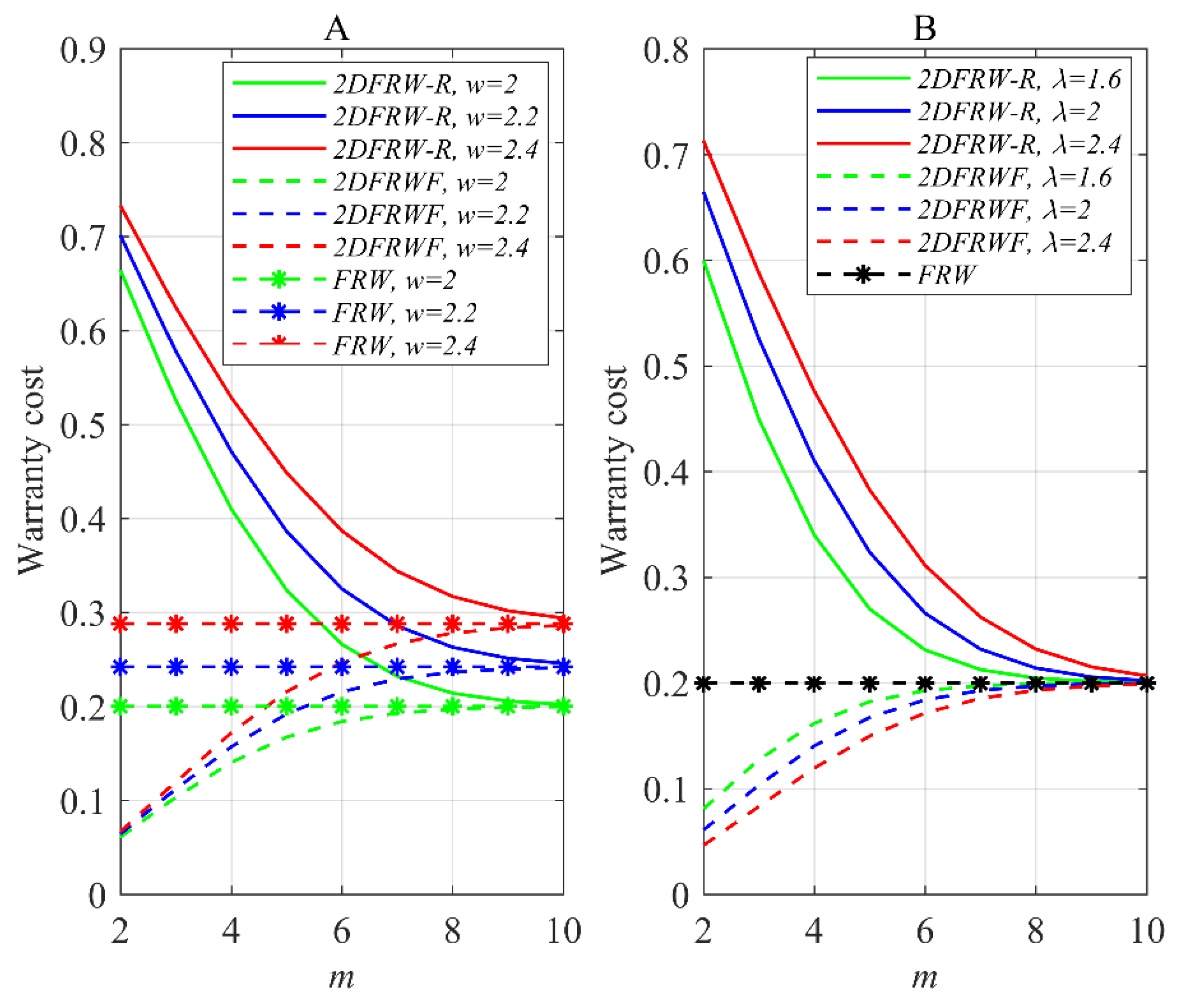
To show how $m$, $w$, and $\lambda$ affect 2DFRW-R, we plot Figure 1 by letting $\alpha =0.5$, $\beta =2$, $a=0.2$, $b=1$, $\kappa =0.8$, $c_R=5$, $c_m=0.1$ and $c_p=12$. As shown in Figure 1A (where $\lambda =1$), for a fixed $w$, the increases in the warranty limit $m$ decrease the warranty cost of 2DFRW-R to the warranty cost of FRW, which is obtained by computing $\underset{m\to \infty }{\lim }WC$. In addition, Figure 1A indicates that the warranty cost of 2DFRW-R increases with the increase in $w$ for a fixed $m$. The above phenomena signal that the warranty cost of 2DFRW-R is lowered by limiting the size of $m$ and/or by shortening the warranty period $w$. Third, Figure 1A shows that the warranty cost of 2DFRW-R exceeds the warranty cost of 2DFRWF in [26] when the warranty limit $m$ is smaller.

Figure 1B (where $w=2$) shows that when $m$ is smaller, the warranty cost of 2DFRW-R increases with the increase in $\lambda$. This means that the warranty cost of 2DFRW-R can rapidly decline to a lower value by lowering $m$ when all job cycles are smaller (i.e., the case in which $\lambda$ is greater, similarly hereinafter). In addition, Figure 1B shows that no matter how $\lambda$ changes, the warranty cost of 2DFRW-R gradually decreases to the warranty cost of FRW with the increase in $m$.

4.2. Characteristic Analysis of BRPR

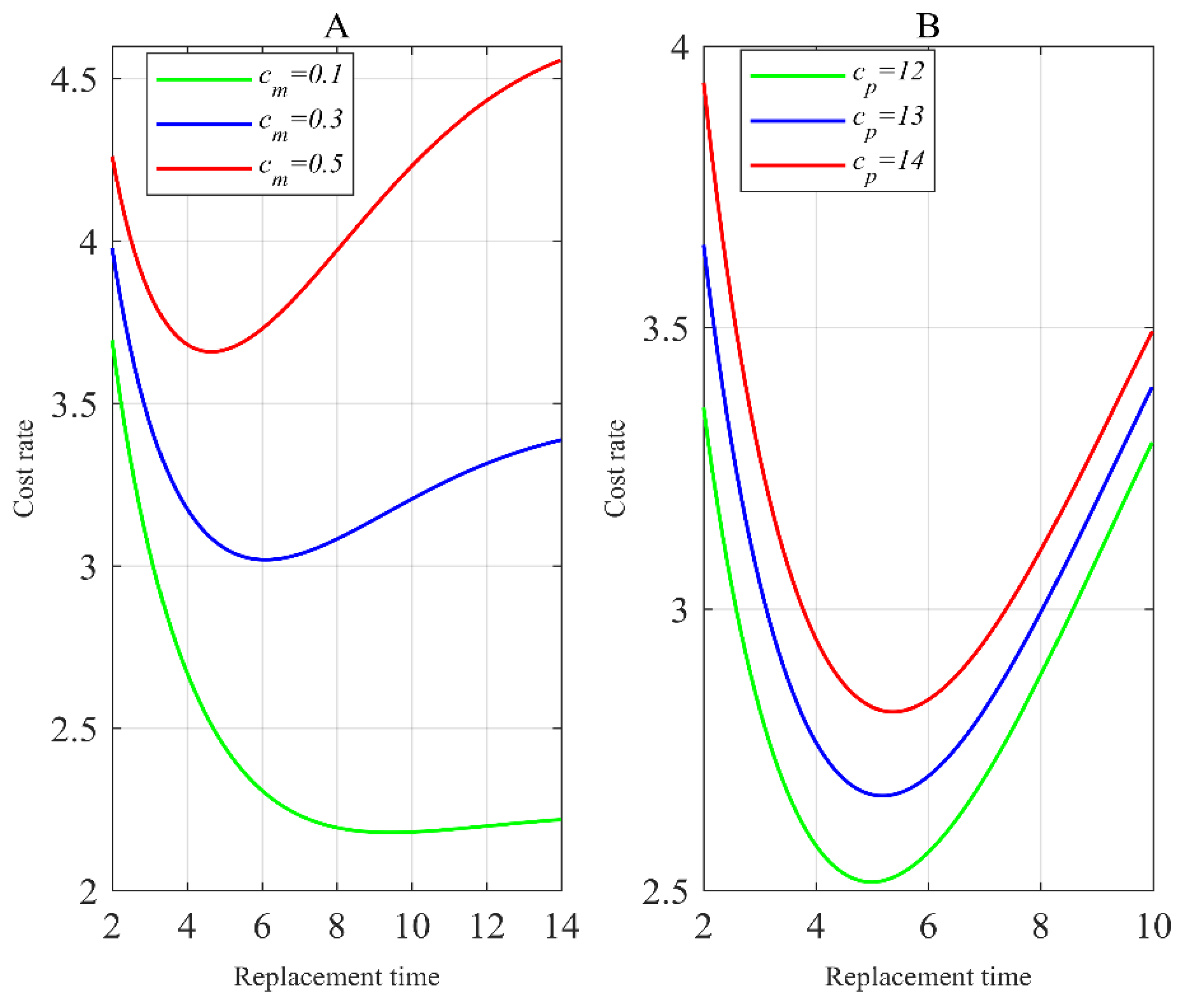
To explore the effect of $c_m$ and $c_p$ on the optimal BRPR, we make Figure 2 by letting $\alpha =0.5$, $\beta =2$, $a=0.2$, $b=1$, $\kappa =0.8$, $m=2$, $c_R=5$, $\lambda =1$ and $w=2$. Figure 2A (where $c_p=12$ and $N=10$) shows that with the increase in the repair cost $c_m$, the minimum expected cost rate $CR(10,T^{\ast })$ increases while the optimal replacement time $T^{\ast }$ decreases. This indicates that the lower repair cost can reduce the minimum expected cost rate and lengthen the optimal post-warranty service period. Figure 2B (where $c_m=0.1$ and $N=10$) indicates that both the minimum expected cost rate $CR(10,T^{\ast })$ and the optimal replacement time $T^{\ast }$ increase when $c_p$ is increasing. This means that the greater replacement cost $c_p$ is unable to reduce the minimum expected cost rate, but it is able to extend the optimal post-warranty service period.

To explore the effect of $m$ and $\lambda$ on the optimal BRPR, we make

Table 1. Sensitivity analysis.

$\mathit{m}$	$\mathit{\lambda } = 1$			$\mathit{\lambda } = 1.5$			$\mathit{\lambda } = 2$
	${\mathit{T}}^{\ast }$	${\mathit{N}}^{\ast }$	$\mathit{C}\mathit{R}({\mathit{N}}^{\ast },{\mathit{T}}^{\ast })$	${\mathit{T}}^{\ast }$	${\mathit{N}}^{\ast }$	$\mathit{C}\mathit{R}({\mathit{N}}^{\ast },{\mathit{T}}^{\ast })$	${\mathit{T}}^{\ast }$	${\mathit{N}}^{\ast }$	$\mathit{C}\mathit{R}({\mathit{N}}^{\ast },{\mathit{T}}^{\ast })$
5	4.6892	13	2.6676	4.7232	17	2.6435	4.7880	20	2.6074
6	4.6815	13	2.6740	4.6933	17	2.6621	4.7243	20	2.6382
7	4.6798	13	2.6761	4.6832	16	2.6711	4.6958	19	2.6575
8	4.6795	13	2.6767	4.6803	16	2.6749	4.6846	19	2.6681

by letting $\alpha =0.1$, $\beta =3$, $a=0.5$, $b=1$, $\kappa =0.3$, $m=2$, $c_R=10$, $c_m=0.1$, $w=2$ and $c_p=12$.

Table 1 shows that for a given $\lambda$, with the increase in the warranty limit $m$, the minimum expected cost rate $CR(N^{\ast },T^{\ast })$ increases while the optimal replacement time $T^{\ast }$ decreases. Such a phenomenon indicates that a smaller $m$ can reduce the minimum expected cost rate and lengthen the optimal post-warranty service period. As shown in Table 1, for a given $m$, with the increase in $\lambda$, the minimum expected cost rate $CR(N^{\ast },T^{\ast })$ decreases while the optimal replacement time $T^{\ast }$ increases. From the whole perspective, this means that when all job cycles are smaller, the minimum expected cost rate is lowered and the optimal post-warranty service period is extended.

4.3. Comparison

To use largely the remaining life of the product through 2DFRW-R, in this study, we have planned that BRPR sustains the post-warranty reliability. If $N=1$, BRPR is reduced to RPRF in [27], i.e., the post-warranty reliability is sustained by any of the above random periodic replacements. Random periodic replacement with the best performance is an ideal replacement policy. This means that an ideal maintenance policy is chosen by ranking the performance of the above random periodic replacements.

In addition, 2DFRWF in [26] and 2DFRW-R in this study are able to warrant the product. Under these cases, how the above warranties affect the optimal BRPR is an interesting focus.

In this subsection, from the numerical perspective, we provide consumers with a guide for selecting an ideal maintenance policy and explore how the above warranties affect the optimal BRPR.

To compare the performance of BRPR and RPRF and explore the effect of warranties on the optimal BRPR, we take 2DFRW-R and FRW as examples and make Figure 3, where $\alpha =0.1$, $\beta =3$, $\lambda =0.5$, $a=0.5$, $b=1$, $\kappa =0.3$, $c_R=10$, $c_m=0.1$, $w=2$ and $c_p=12$.

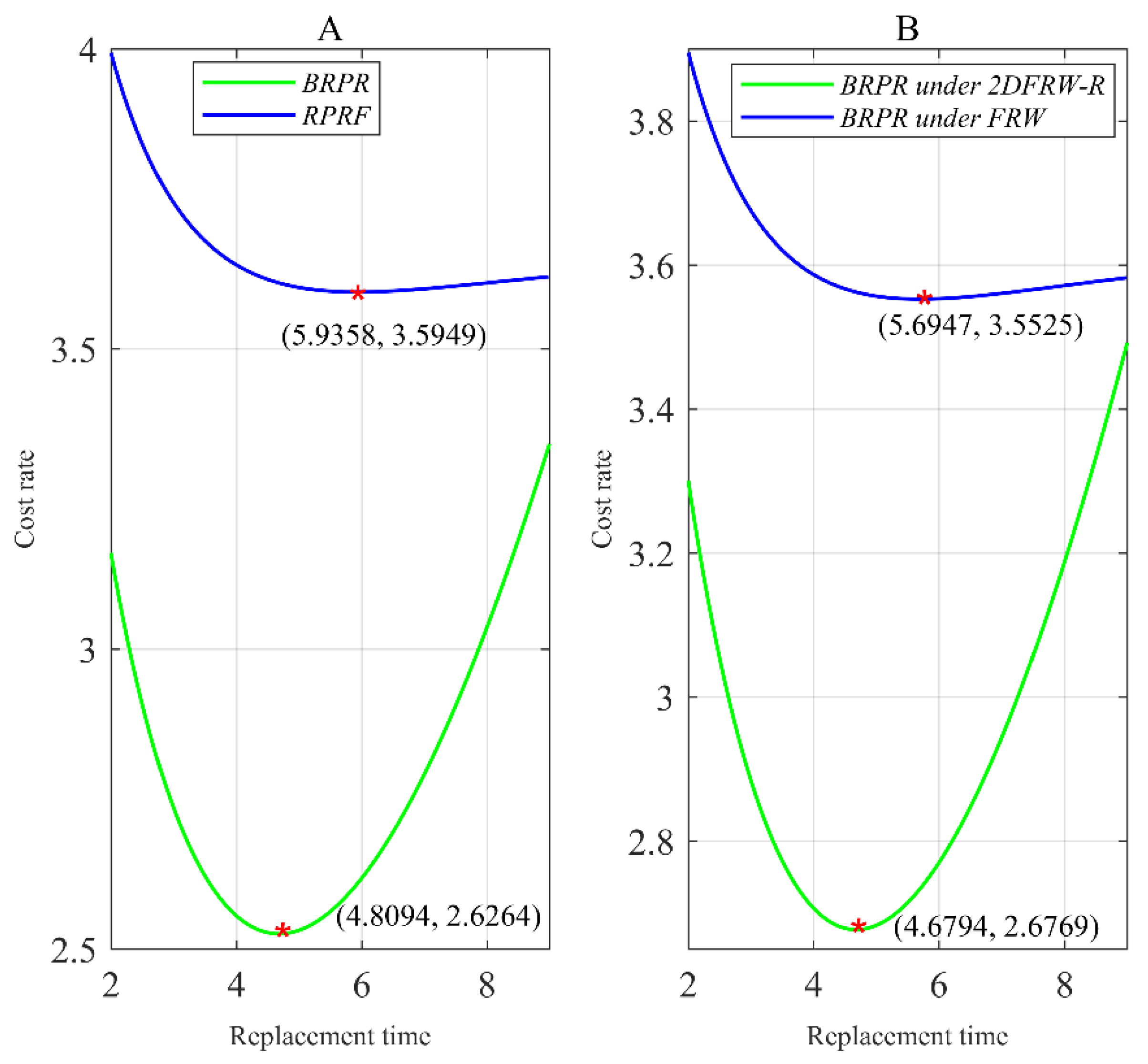
As indicated in Figure 3A (The symbol (*) denotes the minimum point), where $N^{\ast }=10$, the minimum expected cost rate of RPRF exceeds the minimum expected cost rate of BRPR, and the optimal replacement time of RPRF also exceeds the optimal replacement time of BRPR. Because the dimensions are not the same, the above changes mean that the performance of BRPR and RPRF cannot be ascertained in Figure 3A.

Figure 3B shows that the minimum expected cost rate of BRPR under RFW exceeds the minimum expected cost rate of BRPR under 2DFRW-R, and the optimal replacement time of BRPR under RFW also exceeds the optimal replacement time of BRPR under 2DFRW-R. Similarly, the dimensions are not the same, thus these changes still cannot indicate how RFW or 2DFRW-R affect the optimal BRPR.

Next, we rank random periodic replacements by means of the numerical method below. We take BRPR and RPRF as examples.

Let $LCC(N^{\ast },T^{\ast })$ and $LCC(1,T^{\ast })$ be the optimal values of the total costs during the life cycle, which are related to BRPR and RPRF, respectively. Furthermore, denote $L(N^{\ast },T^{\ast })$ and $L(1,T^{\ast })$ by the optimal values for the lengths of the life cycles related to both. Third, let $L_N^{\ast \ast }$ and $L_o^{\ast \ast }$ be the cycle lengths related to both, under the condition at which the total costs of two random periodic replacements are multiplicative. Then, the numerical method below is presented.

Step 1:Letting$L_N^{\ast \ast }=LCC(1,T^{\ast })\cdot L(N^{\ast },T^{\ast })$ and $L_o^{\ast \ast }=LCC(N^{\ast },T^{\ast })\cdot L(1,T^{\ast })$;

Step 2:BRPR is an ideal maintenance policysustaining the post-warranty reliability if$L_N^{\ast \ast }>L_o^{\ast \ast }$; RPRF is an ideal maintenance policysustaining the post-warranty reliability if$L_o^{\ast \ast }>L_N^{\ast \ast }$; every of them is able to sustain the post-warranty reliability whose key cause is that their performance is equivalent if$L_o^{\ast \ast }=L_N^{\ast \ast }$.

By means of the numerical method, we next determine the rank of random periodic replacements under 2DFRW-R.

Let $\alpha =0.1$, $\beta =3$, $\lambda =0.5$, $a=0.5$, $b=1$, $\kappa =0.3$, $c_R=10$, $\lambda =0.5$, $c_m=0.1$ and $c_p=12$; we make

Table 2. Performance comparison ($m=2$).

$\mathit{w}$	2RPR		RPRF		Cycle Lengths
	$\mathit{L}({\mathit{N}}^{\ast },{\mathit{T}}^{\ast })$	$\mathit{L}\mathit{C}\mathit{C}({\mathit{N}}^{\ast },{\mathit{T}}^{\ast })$	$\mathit{L}(1,{\mathit{T}}^{\ast })$	$\mathit{L}\mathit{C}\mathit{C}(1,{\mathit{T}}^{\ast })$	${\mathit{L}}_{\mathit{N}}^{\ast \ast }$	${\mathit{L}}_{\mathit{o}}^{\ast \ast }$
0.5	6.6492	17.6397	2.4708	12.7955	85.0798	43.5842
0.8	6.6317	17.5057	2.7466	12.8288	85.0768	48.0812
1	6.6236	17.4439	2.9226	12.8726	85.2630	50.9815
1.5	6.6100	17.3565	3.3308	13.0404	86.1970	57.8110
2	6.6020	17.3395	3.6899	13.2648	87.5742	63.9810

. As shown in Table 2, the cycle length $L_N^{\ast \ast }$ is longer than the cycle length $L_o^{\ast \ast }$, i.e., $L_N^{\ast \ast }>L_o^{\ast \ast }$, when $w$ is the same. This means that BRPR’s performance is better than RPRF’s performance, i.e., compared with RPRF, BRPR in this study can largely use the remaining life of the product through 2DFRW-R.

Next, we make the symbol assumption similar to Table 2 and use the numerical method to explore how 2DFRW-R and FRW affect the optimal BRPR. We make

Table 3. Performance comparison ($m=\infty$).

$\mathit{w}$	2RPR under 2DFRW-R		2RPR under FRW		Cycle Lengths
	${\mathit{L}}_{\mathit{P}\mathit{W}}({\mathit{N}}^{\ast },{\mathit{T}}^{\ast })$	$\mathit{L}\mathit{C}{\mathit{C}}_{\mathit{P}\mathit{W}}({\mathit{N}}^{\ast },{\mathit{T}}^{\ast })$	${\mathit{L}}_{\mathit{F}\mathit{R}\mathit{W}}({\mathit{N}}^{\ast },{\mathit{T}}^{\ast })$	$\mathit{L}\mathit{C}{\mathit{C}}_{\mathit{F}\mathit{R}\mathit{W}}({\mathit{N}}^{\ast },{\mathit{T}}^{\ast })$	${\mathit{L}}_{\mathit{P}\mathit{W}}^{\ast \ast }$	${\mathit{L}}_{\mathit{F}\mathit{R}\mathit{W}}^{\ast \ast }$
0.5	6.6962	17.9920	2.4763	13.0392	87.3131	44.5536
0.8	6.7020	17.9714	2.7656	13.1612	88.2064	49.7017
1	6.7085	17.9479	2.9568	13.2447	88.8521	53.0684
1.5	6.7384	17.8568	3.4292	13.4617	90.7103	61.2345
2	6.7888	17.7194	3.8926	13.6825	92.8878	68.9745

by letting $\alpha =0.1$, $\beta =3$, $\lambda =0.5$, $a=0.5$, $b=1$, $\kappa =0.3$, $c_R=10$, $\lambda =0.5$, $c_m=0.1$ and $c_p=12$. As indicated in Table 3, the cycle length $L_{PW}^{\ast \ast }$ is longer than the cycle length $L_{FRW}^{\ast \ast }$, i.e., $L_{PW}^{\ast \ast }>L_{FRW}^{\ast \ast }$, when $w$ is the same. This means that the performance of BRPR under 2DFRW-R is better than that of BRPR under FRW. In other words, compared with FRW, 2DFRW-R is able to lengthen the optimal post-warranty service period and lower the minimum expected cost rate.

5. Conclusions

By integrating both limited job cycles and a refund into classic free repair warranty, in this study, a warrantor’s two-dimensional free repair warranty with a refund (2DFRW-R) is presented to help warrantors ensure product reliability and guarantee fairness to consumers. The related warranty cost is derived, and the characteristics of 2DFRW-R are illustrated from the points of view of the warrantor and consumer. By extending the accomplishment of a job cycle to the accomplishment of the $N\mathrm{th}$ job cycle, a bivariate random periodic replacement (BRPR) model is investigated to sustain the post-warranty reliability and use largely the remaining life of the product that goes through warranty. The expected cost rate is constructed for BRPR, and some special models are derived by simplifying the cost rate model. Sensitivities in some of the parameters of both 2DFRW-R and BRPR are analyzed in numerical examples. It is shown that compared with univariate random periodic replacement, BRPR can largely use the remaining life of the product that goes through warranty.

In addition, some other problems could also be investigated in the future, as shown below.

• Some two-dimensional renewing warranty models could be defined and modeled by incorporating limited job cycles into traditional renewing warranty models.
• By integrating the limited job cycles into the product’s life cycle, the on-condition warranties and maintenances could be modeled.
• By integrating limited job cycles into the life cycle of the multicomponent system, modeling warranties and designing maintenance policies to sustain the post-warranty reliability are two additional research directions.