An Artificial Bee Colony Algorithm for Static and Dynamic Capacitated Arc Routing Problems

Abstract

The Capacitated Arc Routing Problem (CARP) is a combinatorial optimization problem, which requires the identification of such route plans on a given graph to a number of vehicles that generates the least total cost. The Dynamic CARP (DCARP) is a variation of the CARP that considers dynamic changes in the problem. The Artificial Bee Colony (ABC) algorithm is an evolutionary optimization algorithm that was proven to be able to provide better performance than many other evolutionary algorithms, but it was not used for the CARP before. For this reason, in this study, an ABC algorithm for the CARP (CARP-ABC) was developed along with a new move operator for the CARP, the sub-route plan operator. The CARP-ABC algorithm was tested both as a CARP and a DCARP solver, then its performance was compared with other existing algorithms. The results showed that it excels in finding a relatively good quality solution in a short amount of time, which makes it a competitive solution. The efficiency of the sub-route plan operator was also tested and the results showed that it is more likely to find better solutions than other operators.

1. Introduction

The Capacitated Arc Routing Problem (CARP) is an NP-hard combinatorial optimization problem that was first introduced by Golden and Wong in [1]. The CARP requires determining the least cost route plans on a graph of a road network for vehicles subject to some constraints. It has many applications in real life, for instance, in winter gritting [2,3] or in urban solid waste collection [4,5]. Since the CARP is an NP-hard problem, instead of exact methods, mainly heuristics and meta-heuristics (e.g., [6,7,8,9,10]) are considered in the literature to find solutions. The existing methods are either too slow or do not give enough good quality solutions, so there is still room for improvements.

The standard CARP assumes a static problem, which is not the closest to real life, where changes may happen during the execution of the solution. These changes modify the instance, and thus, may have an effect on the feasibility and optimality of the current solution [11]. For this reason, the Dynamic CARP (DCARP), which is a variation of the CARP that takes into account dynamic changes, is a better approach. To make the model of the problem under consideration closer to the real-life problem, the changes should be made based on the collected information about the vehicles and the roads. For instance, information can be provided by the drivers of the vehicles about the executed tasks, by the GPS of the vehicles about their current position, and (indirectly) by traffic patrol drones [12] about the current state of the roads.

The Artificial Bee Colony (ABC) algorithm is a swarm intelligence-based algorithm for optimization problems [13]. It was successfully applied on multiple combinatorial optimization problems that are similar to the CARP [14,15,16,17,18,19] and was shown that the ABC algorithm provides better performance than most of the evolutionary computation-based optimization algorithms [16]. However, the ABC algorithm was never applied before, neither on the CARP nor on the DCARP.

In our previous work [20], we collected all the possible events and analyzed their effects on the model. Based on the results, a data-driven DCARP framework with three event handling algorithms and a rerouting algorithm (RR1) was developed. The framework uses ‘the ‘virtual task” strategy [21] to be able to use static CARP solvers for DCARP instances.

The contributions of this work are as follows:

• The definition of the first ABC algorithm for the CARP (CARP-ABC).
• The definition of a new small step-size move operator for the CARP, the sub-route plan operator, which is utilized in the CARP-ABC algorithm.
• The definition of a new method for creating initial population, the RSG. The purpose of the RSG is to create random but feasible solutions for the CARP quickly.
• Numerical experiments to test the CARP-ABC algorithm on a variety of CARP and DCARP instances. The same experiments were performed with other algorithms for CARP, then the results were compared. The results showed that for both CARP and DCARP instances, the CARP-ABC algorithm excels in finding a relatively good quality solution in a short amount of time.
• Numerical experiments to test the efficiency of the sub-route plan operator within the CARP-ABC algorithm, on a variety of CARP instances. The results showed that the sub-route plan operator is more likely to find a better solution than the other operators, especially when a greater modification is needed on the current solution (since it is a randomly generated solution and/or it is a solution of a larger CARP instance).

The rest of the paper is structured as follows. In Section 2, the related works are presented. In Section 3, the basic concepts related to the proposed CARP-ABC algorithm is introduced. In Section 4 and Section 5, the algorithm and the sub-route plan move operator are formulated in detail, respectively. In Section 6, the experiments and their results are discussed. The paper is concluded in Section 7.

2. Related Works

In this section, the related works are introduced. In Section 2.1, the algorithms that were developed for CARP are presented. In Section 2.2, the approaches for DCARP are summarized. In Section 2.3, the ABC algorithms that were developed for problems that are similar to the CARP are presented.

2.1. Algorithms for the CARP

As it was mentioned in Section 1, there are mainly approximate approaches (i.e., heuristics and metaheuristics) for the CARP. For this reason, only the methods that belong to that category are mentioned in this subsection.

2.1.1. Heuristics

Golden et al. developed the first heuristic algorithms for the CARP, namely, the path-scanning and the augment-merge [22]. Other notable heuristics for the CARP are the parallel-insert method [23], Ulusoy’s tour splitting method [24], the augment-insert method [25], the path-scanning with ellipse rule [26] and the path-scanning with efficiency rule [27].

2.1.2. Metaheuristics

The metaheuristic algorithms for the CARP can be divided into two main categories (with some exceptions): trajectory-based and population-based.

From the trajectory-based algorithms, the notable ones are the guided local search algorithm [28], the tabu search algorithms [29,30], the variable neighborhood search algorithm [31], and the greedy randomized adaptive search procedure with evolutionary path relinking [32]. It must be mentioned that in [29], two versions of the tabu search algorithm (TSA) were proposed (TSA1 and TSA2), from which the latter performed better. In [33], a global repair operator was developed and embedded into the TSA, creating the repair-based tabu search (RTS), which outperforms the TSA.

From the population-based algorithms, the notable ones are the genetic algorithm [34], the memetic algorithms [6,35], and the ant colony optimization algorithms [8,36,37]. From these, the Memetic Algorithm with Extended Neighborhood Search (MAENS) [6] is the most popular one, even though it only gives relatively good quality solutions and also has slow runtime. There are multiple solutions that try to improve some parts of the MAENS (e.g., [9,10]), but these improvements do not really increase the overall performance of it. The Ant Colony Optimization Algorithm with Path Relinking (ACOPR) [8] gives only relatively good quality solutions, but currently it has the fastest runtime on most of the CARP instances from the benchmark test sets.

The Hybrid Metaheuristic Approach (HMA) [7] is a population-based algorithm that utilizes a randomized tabu thresholding procedure as a part of its local refinement procedure. The HMA gives the best quality solutions among all existing algorithms and has faster runtime than MAENS, but it is still relatively slow on some real-life based CARP instances. The ACOPR gives only relatively good quality solutions, but currently, it has the fastest runtime on most of the CARP instances from the benchmark test sets.

2.2. Approaches for the DCARP

Despite the importance of the DCARP, the number of studies about CARP (or ARP) that consider dynamic changes in the problem during the execution of the solution are relatively small [20,21,38,39,40,41,42,43,44,45]. Moreover, there are only three studies that consider more than two type of changes [20,21,42] and only two of them (including our previous work) considers all the critical changes that can happen [20,21]. (For a more detailed comparison see [11,20].) Critical changes or events may change the problem to such an extent that the current solution is not feasible anymore, so handling them is essential. Both [20,21] propose a framework for the DCARP that, instead of using complex specialized algorithms, allows the use of any static CARP solvers for solving a DCARP instance.

To the best of our knowledge, the data-driven solution for the DCARP introduced in [20] is the only data-driven approach for DCARP or even CARP.

2.3. The ABC Algorithm and Its Applications

The original ABC algorithm was proposed by Karaboga in [13]. In [46], Karaboga and Görkemli proposed a new definition for the search behavior of the onlooker bees, which improved the convergence performance of the algorithm. For this reason, the new version of the ABC algorithm was named quick ABC (qABC).

The ABC algorithm was introduced as an algorithm for multivariable and multi-modal continuous function optimization, but later it was successfully applied on other types of optimization problems as well. Karaboga and Görkemli introduced an ABC and a qABC algorithm for combinatorial problems (CABC and qCABC, respectively) and applied them to the Traveling Salesman Problem (TSP) [14,15]. Both algorithms use the Greedy Sub Tour Mutation (GSTM) operator [47], which was developed to increase the performance of a genetic algorithm (GA) that solves the TSP. It was proven that the GSTM is significantly faster and and more accurate than other existing mutation operators [47]. Furthermore, it was shown that the ABC and the qABC algorithm provide better performance than many evolutionary computation-based optimization algorithms [16]. Since the TSP is similar to the CARP, in the hope that an ABC algorithm with a mutation operator such as GSTM will perform well, we developed the CARP-ABC algorithm (Section 4) with the sub-route plan operator (Section 5).

There are also ABC algorithms for the Vehicle Routing Problem (VRP) [48] and its variations [17,18]. However, there is only one ABC algorithm for the CARP and even that is for just a variation of CARP, the undirected CARP with profits [19]. Therefore, to the best of our knowledge, currently there are no ABC algorithms, neither for the CARP nor for the DCARP.

3. Problem Formulations

This section introduces basic concepts related to the proposed CARP-ABC algorithm to help to understand how it works. The concepts are introduced only briefly, for a more detailed description the corresponding works are referred to.

In this section, first, the static CARP, then the (data-driven) DCARP is formulated. It is followed by the introduction of the basic ABC algorithm and the existing move operators for CARP (which are used in the proposed CARP-ABC solution). The notations used for the CARP and the DCARP are collected in

Table A1. Notations used in the CARP and the DCARP.

Notation	Meaning
G	graph $G=(V,A)$
V	set of vertices
$v_0$	the depot $(v_0\in V)$
A	set of arcs
T	set of tasks ($T\subseteq A$)
$t_0$	the dummy task $t_0=(v_0,v_0)$
n	the number of tasks that have to be executed
$inv\left(a\right)$	the inverse of arc $a\in A$
$head\left(a\right)$	the head vertex of arc $a\in A$
$tail\left(a\right)$	the tail vertex of arc $a\in A$
$dc\left(a\right)$	the dead-heading cost of arc $a\in A$
$id\left(t\right)$	the identifier of the task $t\in T$
$dem\left(t\right)$	the demand of task $t\in T$
$sc\left(t\right)$	the serving cost of task $t\in T$
$mdc(v_i,v_j)$	the minimal total dead-heading cost from vertex $v_i$ to $v_j$ ($v_i,v_j\in V$)
w	the number of vehicles
q	the maximum capacity of a vehicle
$r_k$	the k-th route plan
$l_k$	the number of tasks on the k-th route plan
$t_{(}k,i)$	the i-th task in the k-th route plan
$DC\left(r_k\right)$	the total dead-heading cost of the route plan $r_k$
$SC\left(r_k\right)$	the total service cost of the route plan $r_k$
I	a CARP instance
S	a solution for the CARP instance I
$TC\left(S\right)$	the total cost of solution S
$T_v$	set of virtual tasks ($T_v\subseteq T$)
H	set of identifiers of all the vehicles ($\left|H\right|=w$)
$H_f$	set of the identifiers of the (currently) free vehicles ($H_f\subseteq H$)
R	set of identifiers of all the route plans
$R_e$	set of identifiers of the route plans whose execution stopped ($R_e\subseteq R$)
$rt\left(k\right)$	the virtual task of the k-th route plan ($k\in R$, $rt\left(k\right)\in T_v$)
$rv\left(k\right)$	the identifier of the vehicle that is executing the k-th route plan ($k\in R$, $rv\left(k\right)\in H$)
m	the number of DCARP instances within a DCARP scenario
$\mathcal{I}$	a DCARP scenario, a set of DCARP instances ($\left|\mathcal{I}\right|=m$)
$I_i$	the i-th DCARP instance within a DCARP scenario ($0\le i<m$)
$S_i$	the accepted solution for the i-th DCARP instance
$TC\left(S_i\right)$	the total cost of solution $S_i$

in Appendix A.

3.1. The CARP

In the existing works, as the input graph, some assume an undirected graph [7], others assume a directed graph [8,49], and other ones a mixed graph [6,34]. In this work, a directed graph is assumed, in which undirected edges are regarded as two oppositely directed edges.

The (directed) graph of the CARP can be described the following way: $G=(V,A)$, with a set of vertices V and a set of arcs (directed edges) A. A set of tasks $T\subseteq A$ is also given, which defines the arcs that have tasks assigned to them. If the graph of a CARP instance contains (undirected) edges, then an edge is added to A as a pair of arcs, one for each direction. For instance, if $(v_i,v_j)$ is an edge and $v_i,v_j\in V$, then the arcs $(v_i,v_j)$ and $(v_j,v_i)$ are added to A. Similarly, if $(v_i,v_j)$ is an edge with tasks assigned to it and $v_i,v_j\in V$, then the arcs $(v_i,v_j)$ and $(v_j,v_i)$ are added to T. The graph also has a special vertex $v_0$ ($v_0\in V$), the depot, and a dummy task $t_0=(v_0,v_0)$, the significance of which is explained later.

The tasks are performed by a fleet of w homogeneous vehicles of capacity q. Every vehicle starts and ends its route at the depot ($v_0$). Each task must be performed in a single operation, and each vehicle can satisfy at most as many demands as its maximum capacity.

The graph can be mapped to a road network where the arcs are road segments. Some of the road segments have tasks. To fulfill the tasks, different amounts but the same type of demand must be served. Each arc is characterized by the following functions:

• $head$: the head vertex of the arc;
• $tail$: the tail vertex of the arc;
• $dc$: the dead-heading or traversing cost, the cost of crossing the arc.

In addition, each task is characterized by the following functions:

• $id$: the unique identifier of the task, which is a positive integer;
• $dem$: (positive) demand, which indicates the load necessary to serve the task;
• $sc$: service cost, which is the cost of executing the task and crossing the arc (i.e., $dc$ is included in $sc$).

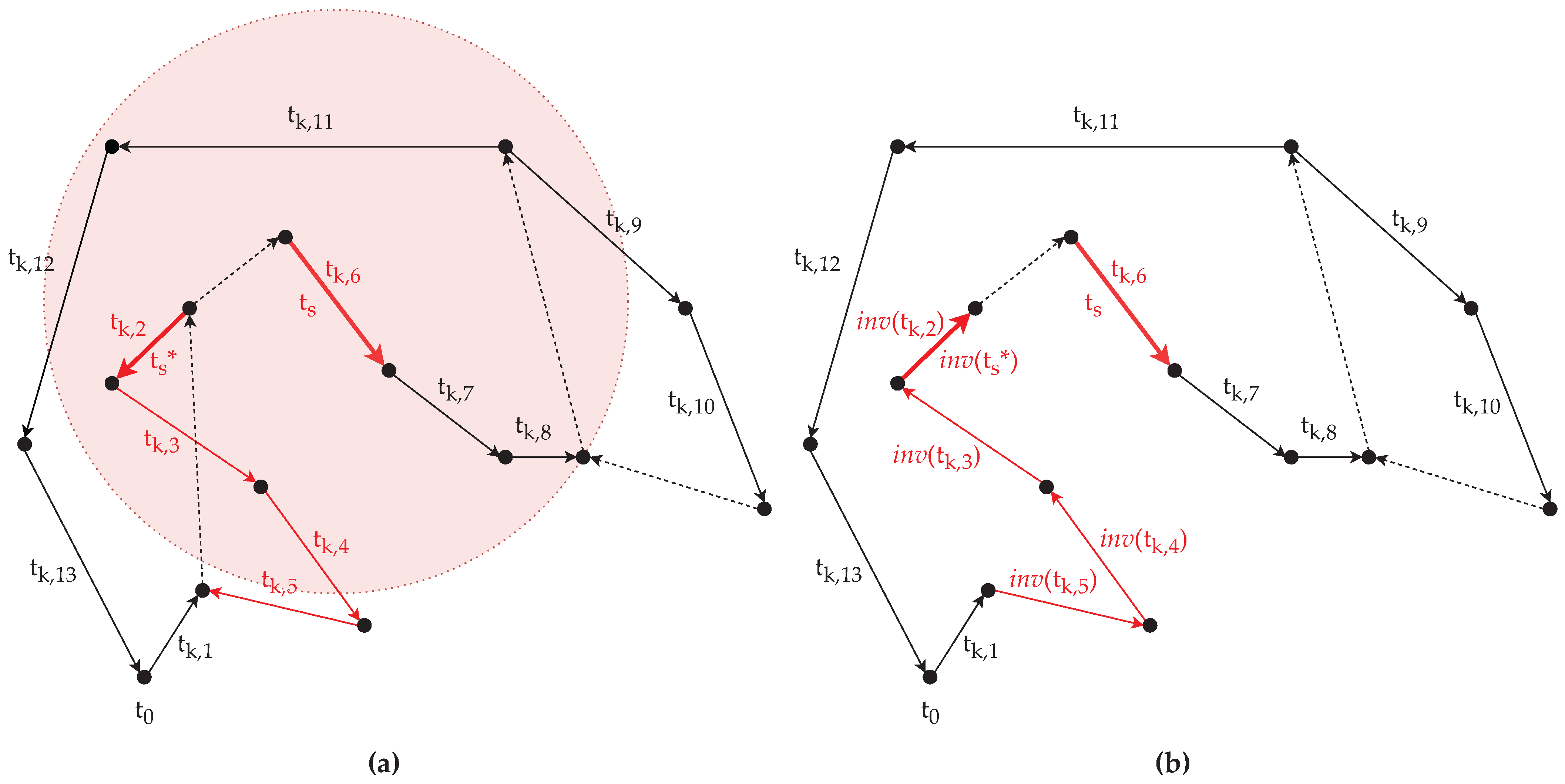
Although an edge is regarded as two oppositely directed arcs, if a task is assigned to it, then the task should be executed only once, in either direction. Let $t\in T$ be a task of one of the arcs of an edge, then let $inv\left(t\right)$ denote the inversion of t, the other task of the edge. If $head\left(t\right)$ and $tail\left(t\right)$ are the head and the tail vertexes of t, then $head\left(inv\right(t\left)\right)=tail\left(t\right)$ and $tail\left(inv\right(t\left)\right)=head\left(t\right)$ are the head and the tail vertexes of $inv\left(t\right)$. The $dc$, $dem$ and $sc$ values are the same for t and $inv\left(t\right)$.

Let the total number of tasks that have to be executed by at least one of the vehicles be denoted by n. The value of n depends on the composition of T: if T only contains arc tasks from edges, then $n=\left|T\right|/2$, if T only contains arc tasks from arcs then $n=\left|T\right|$.

The minimal total dead-heading cost between two vertices is provided by the $mdc:V\times V\to N$ function, which uses Dijkstra’s algorithm as the search algorithm. For instance, $mdc(v_i,v_j)$ denotes the minimal total dead-heading cost traversing from vertex $v_i$ to vertex $v_j$, where $v_i,v_j\in V$.

A CARP instance (I) is defined as follows:

$$I=(V,v_0,A,T,n,w,q,head,tail,dc,id,dem,sc,inv,mdc)$$

(1)

3.1.1. Solution Representation

A solution for a CARP instance is expressed as a set of route plans. The route plans are sequences of the $t\in T$ tasks that need to be executed in the given order. The consecutive tasks are connected by the shortest paths, which is provided by the $mdc$ function. Therefore, a solution S for a CARP instance can be expressed the following way:

$$S=\{r_1,r_2,\dots ,r_{\left|S\right|}\}$$

(2)

where $\left|S\right|$ is the number of route plans and $r_k$ ($k\in \{1,2,\dots ,|S\left|\right\}$) is the k-th route plan within the solution S. The k-th route plan can be expressed the following way:

$$r_k=\langle t_0,t_{k,1},t_{k,2},\dots ,t_{k,l_k},t_0\rangle$$

(3)

where $l_k$ is the number of (not dummy) tasks and $t_{k,i}$ is the i-th task within the k-th route plan. It must be noted that here, k is an index, which is only used to identify a specific route plan in the solution. The order of the route plans within the solution has no effect on the quality of the solution.

Since every route starts and ends in the depot, the dummy task $t_0$ – which represents the vehicle being in the depot – is added also as the first and the last element of the route plan sequences. Its $id$, $dc$, $dem$ and $sc$ are set to 0, and both the head and the tail vertexes are the depot vertex.

For the solution representation of the CARP, a natural encoding approach can be used, just like in most vehicle routing problems. This means that all route plans can be encoded as an ordered list of ids of the tasks, so a solution can be represented as the concatenation of these lists. However, every route plan starts and ends with the dummy task $t_0$, so if the encoded route plans are concatenated, then there are consecutive dummy tasks in the resulting list. For the sake of simplicity, only one of each consecutive dummy task is kept in the encoded solution. Figure 1 shows an example of a solution representation.

3.1.2. Objective and Constraints

The objective of the CARP is to minimize the total cost of the solution S subject to some constraints, which are defined in this section. The total cost of a solution S (i.e., $TC\left(S\right)$) is calculated with the following formula (Equations (4)–(6)):

$$TC\left(S\right)=\sum _{k=1}^{\left|S\right|}DC\left(r_k\right)+SC\left(r_k\right)$$

(4)

$$DC\left(r_k\right)=mdc\left(t_0,head\left(t_{k,1}\right)\right)+\sum _{i=1}^{l_k-1}mdc\left(tail\left(t_{k,i}\right),head\left(t_{k,i+1}\right)\right)+mdc\left(tail\left(t_{k,l_k}\right),t_0\right)$$

(5)

$$SC\left(r_k\right)=\sum _{i=1}^{l_k}sc\left(t_{k,i}\right)$$

(6)

where $DC\left(r_k\right)$ and $SC\left(r_k\right)$ are the total dead-heading and service cost of the route plan $r_k$.

The solution S has to satisfy the following constraints. First, each route plan starts and ends at the depot. Second, each task is executed exactly once. Therefore, the total number of tasks executed on each route plan (excluding the dummy task $t_0$) is equal to n:

$$\sum _{k=1}^{\left|S\right|}{l}_k=n$$

(7)

Moreover, a task cannot be executed more than once, neither in the same route nor in another route:

$$t_{a,i}\ne t_{b,j},\forall (a,i)\ne (b,j)$$

(8)

where $r_a$ and $r_b$ are route plans within S, $t_{a,i}$ is the i-th task in the route plan $r_a$, and $t_{b,j}$ is the j-th task in the route plan $r_b$. If a task t has an inverse (i.e., $\exists inv\left(t\right)$), then either t or $inv\left(t\right)$ is executed. Both cannot be executed in the same solution. Third, the total demand served each route plan does not exceed the capacity (q) of the vehicle:

$$\sum _{i=1}^{l_k}dem\left(t_{k,i}\right)\le q,\forall k\in \{1,2,\dots ,|S\left|\right\}$$

(9)

3.2. The Data-driven DCARP

There are various approaches for DCARP, but in this work, the data-driven version of DCARP is considered, which was recently formulated in [20].

In this problem, instead of one static CARP instance, there is a series of DCARP instances (i.e., a DCARP scenario [21]) that needs to be solved. A DCARP scenario is denoted by $\mathcal{I}=\langle I_0,I_1,\dots ,I_i,\dots ,I_{m-1}\rangle$, where m is the number of DCARP instances within the scenario (i.e., the number of dynamic events that occurred and changed the previous DCARP instance is $m-1$). Each $I_i$ ($I_i\in \mathcal{I}$) DCARP instance contains all the information about the current problem. The previous DCARP instance $I_{i-1}$, the execution of the accepted solution for $I_{i-1}$ and the occurred event(s) define the next DCARP instance $I_i$, where $0<i<m$. The initial instance ($I_0$) can be viewed as a static (data-driven) CARP instance, since initially every vehicle is in the depot (in good state) and no task has been executed yet.

For a data-driven DCARP instance, information needs to be stored about all the vehicles and route plans. For each vehicle, the current location and state have to be known. Furthermore, identifiers are needed to be used for the vehicles and the route plans, since a vehicle may follow multiple route plans (one after another) and it is important to know for each route plan whether a vehicle already executed it, its execution is still in progress, or a vehicle still needed to be assigned to it to start its execution.

Instead of the number of vehicles (w), a set of identifiers of all the vehicles is needed to be defined, which is denoted by H. The set of the identifiers of the (currently) free vehicles is denoted by $H_f$ ($H_f\subseteq H$), which is initially equal to H. The identifier of a vehicle is added to $H_f$, if the vehicle finishes the execution of a route plan, and the identifier is removed, when a new route plan is assigned to the vehicle. If the execution of all the tasks is finished and all the vehicles are returned to the depot (i.e., there are no broken down vehicles outside on the roads), then $H_f=H$, otherwise $H_f\subset H$.

The set of identifiers of all the route plans is denoted by R, and the set of identifiers of the route plans that currently cannot be modified and not executed by any vehicle is denoted by $R_e$ ($R_e\subseteq R$). When a new route plan is created, its identifier is added to R, and when the execution of it is finished or suspended (due to vehicle breakdown), its identifier is added to $R_e$. If the execution of all the route plans is finished and there are no more tasks to execute, then $R_e=R$, otherwise $R_e\subset R$. The identifier is removed from $R_e$ only if the vehicle which is assigned to it was broken, but got fixed and can continue the execution of the plan. The function that defines which vehicle is assigned to a specific route plan is denoted by $rv:R\to H$.

To store the current location of the vehicles in the instance, the virtual task strategy introduced in [21] is used, which replaces the executed tasks in each route plan with “virtual tasks”. A “virtual task” is an arc whose $head$ is the depot vertex $v_0$ and $tail$ is the current location of the vehicle, vertex v ($v\in V$). For the sake of simplicity, it is assumed that when an unexpected event occurs, every vehicle is located exactly at a vertex. Since this task is “virtual”, it cannot be traversed, for this reason, it has an infinite traversing cost (i.e., $dc\left(v\right)=\infty$). Furthermore, since it is a “task”, there is a demand and a service cost assigned to it, which are calculated according to the provided data: the service cost is the total cost produced by the vehicle so far (i.e., it is the sum of traversing and serving cost of the arcs that were crossed or served by the vehicle), and the demand is the total demand served by the vehicle so far. A route plan can have at most one virtual task. Therefore, if a route plan already has a virtual task, then it is updated taking into account the arcs traversed and the tasks executed since then by the corresponding vehicle. The set of all virtual tasks is denoted by $T_v$ ($T_v\subseteq T$), and the function that defines which virtual task belongs to a specific route plan is denoted by $rt:R\to T_v$.

The set of arc tasks that need to be executed is denoted by T. If according to the gathered information a task t ($t\in T$) was executed by the vehicle h ($h\in H$), then in the new DCARP instance t needs to be removed from T. Furthermore, the virtual task of the route plan of the vehicle (e.g., $t_{k,v}$, where $rv\left(k\right)=h$ and $t_{k,v}\in T_v$) needs to be updated. The new virtual task is generated in such a way that t is included in it (along with the other tasks the vehicle executed and arcs the vehicle traversed). If t has an inverse (i.e., $\exists inv\left(t\right)$), then it is removed from T as well. Accordingly, the total number of tasks that have to be executed (n) is decreased by one or two.

The initial DCARP instance ($I_0$) is similar to a static CARP instance. The sets of the route plan identifiers (R) and the function $rv$ are created and filled only after the solution is found for $I_0$. The set $H_f$ is initially equal to H, then based on $rv$, all the vehicle identifiers that are assigned to a route plan are removed from $H_f$. At this stage, the sets $R_e$ and $T_v$ are empty sets, therefore the function $rt$ is an empty function as well. According to these, the initial DCARP instance ($I_0$) is defined as follows:

$$I_0=(V,v_0,A,T,n,w,q,H,head,tail,dc,inv,dem,sc,mdc)$$

(10)

The subsequent DCARP instances ($I_i$, where $0<i<m$) are defined as follows:

$$I_i=(V,v_0,A,T,T_v,n,q,H,H_f,R,R_e,rt,rv,head,tail,dc,inv,dem,sc,mdc)$$

(11)

3.2.1. Structure of a Scenario

A new DCARP instance is constructed and added to the DCARP scenario, when an unexpected event happens that changes the current problem to such an extent that it has effect on the currently executed solution. In [21] all the possible events (based on realistic assumptions) were collected and analyzed based on their effect.

It is assumed that the roadmap, the number of vehicles, and the maximum capacity of the vehicles cannot change (at least during the execution of the solution). Therefore, V, $v_0$, A, $head$, $tail$, $inv$, q and H are the same in all the DCARP instances of a DCARP scenario.

It is assumed that roads can become closed/opened (it changes $dc$, thus $mdc$, too), the traffic can decrease/increase (it changes $dc$ and in some cases $sc$, thus $mdc$, too), tasks can get cancelled/added (it changes T, n, $dem$, and $sc$) and vehicles can breakdown/restart (it changes $R_e$), which are unexpected events. The expected events are the events that normally occur during the execution of the solution: a task is executed (it changes T), a vehicle moves (it changes $T_v$, thus $rt$, too), or a vehicle returns to the depot (it changes $H_f$ and in some cases $rv$). The affected components are updated only when a new instance is constructed. If rerouting is performed, then R and $rv$ may change, but the changes are visible only in the next DCARP instance. Therefore, T, $T_v$, n, $H_f$, R, $R_e$, $rt$, $rv$, $dem$, $sc$, $dc$, and $mdc$ may be different among the DCARP instances of a DCARP scenario.

Since due to the unexpected events some components of the DCARP instance change, the optimal solution may change, too. It is one’s choice to construct a new DCARP instance and reroute when there might be a better solution available, but the current solution is still feasible. However, constructing a new DCARP instance and rerouting is necessary when the current solution is not feasible anymore.

3.2.2. Solution Representation

For each DCARP instance, the solution representation is mainly the same as for static CARP instances. The only difference is that if the route plan has a virtual task assigned to it, then the virtual task is the second task within the route plan (since the first task is always the dummy task $t_0$). For instance, if the route plan $r_k=\langle t_0,t_{k,1},t_{k,2},\dots ,t_{k,l_k},t_0\rangle$ has an identifier k ($k\in R$) and there is a virtual task $t_{v,k}$ assigned to it (i.e., $rt\left(k\right)=t_{v,k}$), then $t_{k,1}=t_{v,k}$.

3.2.3. Objective and Constraints

For each DCARP instance, the objective and the constraints are mainly the same, as well as for static CARP instances. The only difference is at the second constraint, which requires that the total number of tasks in the solution S (excluding the dummy task $t_0$) is equal to the sum of the number of tasks that still need to be executed (n) and the total number of virtual tasks ($|T_v|$):

$$\sum _{k=1}^{\left|S\right|}{l}_k=n+\left|T_v\right|$$

(12)

The attributes of a virtual task guarantee that a solver will always place the virtual task right after the dummy task within a route plan of a (nearly optimal) solution, so there is no need to add a constraint regarding it.

3.2.4. Finding a Solution

The data-driven DCARP framework allows rerouting when a critical event (i.e., an unexpected event that may change the feasibility of the current solution) occurs. These events are the task appearance, the demand increased and the vehicle breakdown.

The data-driven DCARP framework allows the use of static CARP solvers by converting the current data-driven DCARP instance into a static CARP instance. After a (sufficiently good) solution is found by the CARP solver, the solution is converted into a data-driven DCARP solution.

Converting a data-driven DCARP instance into a static CARP instance works as follows: the sets of vehicle and route plan identifiers (i.e., H, $H_f$, R, and $R_e$) are omitted, along with the related functions ($rt$ and $rv$). Furthermore, all virtual tasks related to finished and suspended route plans are removed from T. For instance, if $rt\left(k\right)=t_{v,k}$ ($t_{v,k}\in T$) is the virtual task of the route plan with identifier k ($k\in R$) and $k\in R_e$, then $t_{v,k}$ is removed from T (i.e., $T\backslash \left\{t_{v,k}\right\}$).

Converting a static CARP solution into a data-driven DCARP solution works as follows: the virtual tasks that are related to finished and suspended route plans are added to the solution in separate route plans to keep track the total cost of the DCARP scenario. Furthermore, if there are any new route plans within the solution, the framework gives them identifiers and also attempts to assign each of them to a free vehicle. For the other route plans, it can be easily determined which route plan identifier belongs to which route plan, based on the virtual task within them.

3.3. The Basic ABC Algorithm

This section introduces the basic ABC algorithm for combinatorial problems, based on [16]. Just like in the original ABC algorithm [13], the artificial bees are classified into the three groups:

• employed bees, who are exploiting the food sources;
• onlooker bees, who are making the decision about which food source to select;
• scout bees, who are randomly choosing a new food source.

In the ABC algorithm, a food source is corresponded to a solution and the nectar amount of a food source is corresponded to the fitness of a solution.

The ABC algorithm is an iterative process with four phases in total. It begins with the initial phase, then it iterates three bee phases (always in the same order) until a predefined termination criterion is met. In the initial phase, the population is initialized with randomly generated food sources. In the first phase, the employed bee phase, the employed bees are sent to the food sources, where they determine the nectar amounts of the food sources. In the second phase, the onlooker bee phase, the probability value of the sources are calculated based on their nectar amount, then the onlooker bees are sent to the preferred food source to find neighboring food sources and determine their nectar amount. In the third phase, the scout bee phase, the exploitation process of the sources exhausted by the bees are stopped and the scout bees are sent out to randomly discover new food sources within the search area. In each phase, the best food source found so far is memorized. The phases are described in more detail in the subsections below.

3.3.1. Initialization Phase

In the initialization phase, the parameters and the population are initialized. The parameters of the ABC algorithm can be defined as follows:

• $sn$: the number of food sources, which is also the number of the employed bees and onlooker bees (i.e., for every food source, there is only one employed bee);
• $limit$: the number of trials after which a food source is assumed to be abandoned;
• a termination criterion.

The population is initialized by randomly generating $sn$ number of food sources and assigning one employed bees to each of them. The employed bees evaluate the fitness of these solutions.

3.3.2. Employed Bee Phase

At this phase, each employed bee $x_i$ generates a new food source $x_{new}$ in the neighborhood of its current position. Once $x_{new}$ is obtained, it will be evaluated and compared to $x_i$. If the nectar amount of $x_{new}$ is equal to or higher than that of $x_i$, $x_{new}$ replaces $x_i$ and becomes a new member of the population, otherwise $x_i$ is retained. In other words, a greedy selection mechanism is employed between the old and the new candidate solutions.

3.3.3. Onlooker Bee Phase

An onlooker bee evaluates the nectar information taken from all the employed bees and selects a food source $x_i$ depending on its probability value $p_i$ calculated by the following expression:

$$p_i={\displaystyle \frac{fi{t}_i}{{\sum }_{j=1}^{sn}fi{t}_j}}$$

(13)

where $fi{t}_i$ is the nectar amount (i.e., the fitness value) of the i-th food source $x_i$. The higher the value of $fi{t}_i$ is, the higher the probability of that the i-th food source is selected.

Once the onlooker has selected her food source $x_i$, she produces a modification on $x_i$ by using a local search operator. The local search operator randomly selects a position in the neighborhood of $x_i$. As in the case of the employed bees, if the modified food source has a better or equal nectar amount than $x_i$, the modified food source replaces $x_i$ and becomes a new member in the population.

3.3.4. Scout Bee Phase

If a food source $x_i$ cannot be further improved through a predetermined number of trials limit, the food source is assumed to be abandoned, and the corresponding employed bee becomes a scout. The scout produces a food source randomly.

In the basic ABC algorithm, in each cycle, at most one scout bee goes outside to search for a new food source.

3.4. Move Operators for the CARP

In population-based evolutionary algorithms, to enrich the diversity of the population, move operators with different levels of step-size are utilized to generate new, neighboring solutions. These move operators can be divided into two main categories: small step-size operators and large step-size operators. Small step-size operators can modify the position and/or the direction of the tasks within one or two route plans. In contrast, large step-size operators are able to modify more than two route plans. The most commonly used small step-size operators in the literature, which are used in this work as well, are inversion, (single) insertion, swap, and two-opt operators [6,7,8]. In this work, a novel small step-size operator is used as well, the sub-route plan operator, which is introduced in this work, in Section 5. The only large step-size operator used in this work is merge-split, which was introduced in [6]. It is called a large-step-size operator, since it is able to modify more than two route plans.

The inversion and the sub-route operators can only change the direction and the order of the tasks within one route plan, so they do not change the feasibility of the solution. In contrast, the insertion, the swap, and the two-opt operators may change the amount of demand that needs to be served in some of the route plans, so the feasibility of the solution may change, too. For this reason, based on the settings, the output solution of these operators could be different. If infeasible solutions are not accepted and the calculated output solution is infeasible, then the operator returns the original, input solution instead (assuming that the input solution is a feasible solution).

3.4.1. Inversion Operator

The inversion operator randomly selects a task $t\in T$ within the input solution. If this task has an inverse (i.e., $\exists inv\left(t\right)\in T$), then the operator replaces t with $inv\left(t\right)$ within the solution, else it returns the input solution.

3.4.2. Insertion Operator

The insertion operator randomly selects a task $t_1\in T$, then replaces (inserts) it before or after another randomly selected task $t_2\in T$ within the input solution. The selected tasks can be in different route plans or in the same route plan, but they cannot be the same tasks (i.e., $t_1\ne t_2$).

It creates two potential output solutions, based on where $t_1$ is inserted (before or after $t_2$). If $t_1$ has an inverse, then the operator creates other potential output solutions, which contains the inverse task of the task (i.e., $inv\left(t_1\right)$) instead of $t_1$. It selects the solution as the output solution which has the smallest total cost among the potential output solutions.

3.4.3. Swap Operator

The swap operator randomly selects two tasks ($t_1$ and $t_2$, where $t_1,t_2\in T$), then replaces them with each other (i.e., swaps them). Similarly to the insertion operator, the selected tasks can be from the same route plan or different route plans, but they cannot be the same tasks.

It creates potential output solutions, which contain one or two inverse task(s) of the selected tasks instead of the task(s). All the four possible combinations are considered. It selects the solution as the output solution which has the smallest total cost among the potential output solutions.

3.4.4. Two-Opt Operator

The two-opt operator randomly selects two route plans (e.g., $r_1$ and $r_2$) of the solution. Based on the selected two route plans, two cases exist for this move operator. If the selected two route plans are the same (i.e., $r_1=r_2$), then a sub-route plan (i.e., a part of the route plan) is selected randomly and its direction is reversed. If the selected two route plans are different (i.e., $r_1\ne r_2$), then these two route plans are randomly cut into four sub-route plans, and then two new potential output solutions are generated by reconnecting the four sub-route plans and the best one from them is selected. For example, $r_1$ and $r_2$ are cut into sub-route plans $r_{11}$$r_{12}$ and $r_{21}$$r_{22}$, respectively. Two new solutions are generated by connecting them in the following ways: (1) $r_{11}$ with $r_{22}$ and $r_{21}$ with $r_{12}$ and (2) $r_{11}$ with reversed $r_{21}$ and reversed $r_{12}$ with $r_{22}$.

3.4.5. Merge-split Operator

As it was mentioned before, the merge-split operator can make large changes in the solution (e.g., it can modify the order of all the tasks within one or more route plans), so it is considered a large step-size operator. This operator randomly selects x number of different route plans in the input solution, where x is a random number ($1\le x\le \left|S\right|$). It obtains an unordered list of tasks by merging the tasks of the selected route plans into one list, and then sorts this unordered list with a path scanning heuristic (e.g., [22], which is used in this work as well). The obtained ordered list is then optimally split into new route plans using Ulusoy’s splitting procedure [24].

The ordered list is constructed by the path scanning heuristic the following way. First, an empty path is initialized, then, the affected tasks are added one by one into the current path, until no tasks are left in the unordered list. In each iteration, only those tasks are taken into account that can be added to the current path without breaking the capacity constraint. If there are no any tasks like that, then the depot is added to the current path and a new path is initialized (that becomes the current path). When a task or the depot is added to the current path, the task/depot is connected to the end of the current path with the shortest path between them. If there are multiple tasks that can be added, the one that is closest to the end of the current path is added. If there are multiple tasks that are closest to the end of the current path, then one of the following rules are applied to determine which task should be added next:

1.

maximize the distance between $head\left(t\right)$ and $v_0$;

2.

minimize the distance between $head\left(t\right)$ and $v_0$;

3.

maximize the term $\frac{dem\left(t\right)}{sc\left(t\right)}$;

4.

minimize the term $\frac{dem\left(t\right)}{sc\left(t\right)}$;

5.

use rule 1, if the vehicle is less than half-full, otherwise use rule 2.

In the rules above, t ($t\in T$) is a task and $v_0$ ($v_0\in V$) is the depot. In one run, only one of the rules can be used. Therefore, the path scanning heuristic is ran five times, which results in five ordered lists.

The Ulusoy’s splitting procedure creates five new candidate output solutions from the five ordered lists by splitting the lists into route plans. How the procedure works is best summarized in [50]. The procedure starts with constructing the Directed Acyclic Graph (DAG) from the ordered list. A DAG is a graph with arcs that represent feasible sub-tours of one giant tour. Next, the shortest path through the graph is calculated, which gives the optimal partition of the giant tour into feasible route plans. As the final step, a new candidate solution is created from the untouched route plans of the input solution and the route plans returned by the procedure. From the five candidate solutions the best one is chosen and returned by the operator.

4. The Proposed ABC Algorithm for CARP (CARP-ABC Algorithm)

In this chapter, the ABC algorithm developed for CARP (CARP-ABC algorithm) is presented. The notations used for the CARP-ABC algorithm are collected in

Table A2. Notations used in the CARP-ABC algorithm.

Notation	Meaning
$n_{cs}$	the size of the colony
$n_{mi}$	the maximum number of iterations
$n_{gsl}$	the global search limit
$n_{lsl}$	the local search limit
$n_{sal}$	the solution age limit (within the population)
C	the current colony, a set of solutions ($C=\{S_1,S_2,\dots \}$, $\left|C\right|=n_{cs}$)
$\overline{C}$	the previous colony
$\mathcal{A}$	set of the age of the solutions within C ($\mathcal{A}=\{{\alpha }_1,{\alpha }_2,\dots \}$, $\left|\mathcal{A}\right|=n_{cs}$)
P	set of probability values of the solutions within C ($P=\{p_1,p_2,\dots \}$, $\left|P\right|=n_{cs}$)
I	a CARP instance
$S^{*}$	the currently known globally best solution
$S^{\prime }$	the best solution found within one iteration
$S_i^{*}$	the best solution found in the neighborhood of $S_i\in C$
$S_i^{\prime }$	the best solution found within one iteration, in the neighborhood of $S_i\in C$
$S_{i,j}^{*}$	the best solution found in the neighborhood of $S_{i,j}$ ($S_{i,j}$ is a neighbor of $S_i\in C$)
$S_{i,j}^{\prime }$	the best solution found within one iteration, in the neighborhood of $S_{i,j}$ ($S_{i,j}$ is a neighbor of $S_i\in C$)
${\alpha }^{*}$	the current age of $S^{*}$
${\alpha }^{\prime }$	the current age of $S^{\prime }$
${\alpha }_i^{*}$	the current age of $S_i^{*}$
${\alpha }_i^{\prime }$	the current age of $S_i^{\prime }$

in Appendix A.

The algorithmic description of the main CARP-ABC algorithm can be seen in Algorithm 1. The main algorithm can be divided into four main phases: initialization, employed bee, onlooker bee, and scout bee phases. The algorithm begins with the initialization phase, then enters a cycle, where it repeats the mentioned phases in the respective order until the termination criterion is satisfied (line 4). In the initialization phase (line 2), the colony (C), the age of the solutions within the colony ($\mathcal{A}$), the global best solution ($S^{*}$), and its age (${\alpha }^{*}$) are initialized. In the employed bee phase (line 6), local search is performed around the members of the colony. In the onlooker bee phase (line 7), a more in-depth local search is performed around one solution from the colony. In the scout bee phase (line 8), global search is performed.

Algorithm 1: Main CARP-ABC algorithm.

The parameters of the algorithm are the followings:

• I: a CARP instance;
• $n_{cs}$: the size of the colony, the number of solutions in the population;
• $n_{mi}$: the maximum number of iterations of the algorithm;
• $n_{gsl}$: the global search limit, the maximally allowed number of consecutive iterations in which the currently known global best solution is not improved;
• $n_{lsl}$: the local search limit, the maximally allowed number of consecutive iterations in which the currently known local best solution is not improved in the employed bee phase and the onlooker bee phase of the algorithm;
• $n_{sal}$: the solution age limit, the maximally allowed number of consecutive iterations of the algorithm in which a solution is kept in the population;
• a termination criterion, which in default is that either the $n_{mi}$ or the $n_{gsl}$ is reached.

4.1. Initialization Phase

The algorithmic description of the initialization phase of the CARP-ABC algorithm can be seen in Algorithm 2. The algorithm in this phase first initializes the sets for the solutions $S_i$ for $i=1,2,\dots ,n_{cs}$ and their age (lines 2–3). To guarantee an initial population with certain quality and diversity, the solutions are generated randomly by using the Random Solution Generation (RSG) algorithm for CARP (line 6), which is introduced in this work (in Section 4.1.1). Other population based evolutionary algorithms usually use the Randomized Path-Scanning Heuristic (RPSH) [22] to generate initial solutions. However, our experiments showed that, in the case of the CARP-ABC algorithm, it does not improve the convergence speed of the algorithm, so only the RSG is used.

After the initialization of the colony, the algorithm selects the solution $S_i\in C$ with the best (highest) fitness value by using the $selectBestSolution$ function (line 11). The fitness of a solution $S_i$ is defined by its total cost $TC\left(S_i\right)$ (it needs to be as small as possible). Therefore, the fitness value of a solution $S_i$ is computed by the following fit function:

$$fit\left(S_i\right)={\displaystyle \frac{LB}{TC\left(S_i\right)}}$$

(14)

where $LB$ is the lower bound of the solution (i.e., the total service cost of all the tasks, involving only one of each tasks which has an inverse). Its value ranges between 0 and 1. Solutions with greater fitness values are preferred, since greater fitness value means that the total cost of the solution is closer to the lower bound.

Algorithm 2: initializationP (Initialization Phase of the CARP-ABC algorithm).

4.1.1. Random Solution Generation Algorithm

As the first step, the algorithm generates $n_{cs}$ random permutations, which contain positive integers from 1 to n (i.e., the id of every arc task and one of the two $id$s of every edge task) in random order. As the next step, the algorithm reads the $id$s in the permutation one-by-one from left to right, while summing up the demand of the corresponding tasks. If the task assigned to the currently read $id$ would break the capacity constraint of the current route plan, the algorithm inserts a “0” (the $id$ of the dummy task $t_0$) before the $id$ of the task in the sequence (i.e., the task is added to a new route plan). After it is finished with separating the $id$s of the tasks into route plans, the algorithm checks each task in the solution and, if it has an inverse task, then randomly (e.g., with 0.5 probability) replaces the id of the task with the $id$ of its inverse. As the final step, the algorithm inserts a “0” as the first and last task of the solution to make it a valid solution.

4.2. Employed Bee Phase

The algorithmic description of the employed bee phase of the CARP-ABC algorithm can be seen in Algorithm 3. The algorithm in this phase, for each employed bee, generates new candidate solutions in the neighborhood of $S_i$ with each small step-size operator, then evaluates and selects the best solution (lines 2–11). In this phase, only the inversion operator (line 6) and the sub-route plan operator (line 7) are used, because only these operators guarantee that the new candidate solution will be feasible. It is repeated until the known best local solution $S_i^{*}$ cannot be improved within the defined number of iterations (i.e., its age reached $n_{lsl}$). If the fitness value of the new candidate solution $S_i^{*}$ is greater than or equal to the fitness value of the current solution $S_i$, the new solution replaces the current one in the population (lines 14–15).

As the next step, the algorithm calculates the winning probability values $p_i$ for the solutions $S_i$ (lines 16–19). The probability values $p_i$ are calculated with the same function as in the basic ABC algorithm (Equation (13)).

Algorithm 3: employedBP (Employed Bee Phase of the CARP-ABC algorithm).

4.3. Onlooker Bee Phase

The algorithmic description of the onlooker bee phase of the CARP-ABC algorithm can be seen in Algorithm 4. The algorithm in this phase, depending on the $p_i$ values, selects a solution $S_i$ with the $selectSolution$ function. This function first performs a roulette selection $Int\left(\sqrt{n_{cs}}\right)$ times to select $Int\left(\sqrt{n_{cs}}\right)$ number of solutions from the colony. Next, it compares the selected solutions to each other and selects the best one from them (i.e., the one with the greatest fitness value).

As a next step, the algorithm generates $n_{cs}$ number of new candidate solutions $S_{i,j}$ in the neighborhood of $S_i$ (i.e., one solution for each onlooker bee) with the merge-split operator (lines 5–6). It generates new candidate solutions in the neighborhood of these solutions with the small step-size operators, until the known best local solution $S_{i,j}^{*}$ cannot be improved within the defined number of iterations (i.e., the age of the solution, ${\alpha }_{i,j}^{*}$, reaches $n_{lsl}$) (lines 7–21). In this phase, all the small step-size operators (i.e., inversion, insertion, swap, 2-opt, and sub-route plan) are applied to $S_{i,j}^{\prime }$, which is the best solution that was found in the previous iteration (lines 11–15). From the resulted solutions, the best one is chosen with the $selectBestSolution$ function as the new $S_{i,j}^{\prime }$ (line 16). If the new $S_{i,j}^{\prime }$ is better than the currently known best solution in the neighborhood of $S_{i,j}$ (i.e., $S_{i,j}^{*}$), then it is set as the new best solution $S_{i,j}^{*}$ (lines 17–19). Otherwise, the age of $S_{i,j}^{*}$ (i.e., ${\alpha }_{i,j}^{*}$) is increased by one (lines 20–21). After the search ends in the neighborhood of $S_{i,j}$, it is checked whether the best solution found (i.e., $S_{i,j}^{*}$) is better than the best solution found in the whole neighborhood of $S_i$ (i.e., $S_i^{*}$). If $S_{i,j}^{*}$ has a higher fitness value and is also feasible (its total excess demand is zero), then it will be set as the new $S_i^{*}$ (lines 22–23).

If the best solution found in this phase (i.e., $S_i^{*}$) is better than the current solution $S_i$, then $S_i$ is replaced by $S_i^{*}$ in the colony (lines 25–26).

Algorithm 4: onlookerBP (Onlooker Bee Phase of the CARP-ABC algorithm).

4.4. Scout Bee Phase

The algorithmic description of the scout bee phase of the CARP-ABC algorithm can be seen in Algorithm 5. The algorithm in this phase increases the age of unchanged solutions (lines 3–4) and sets the age to zero for new solutions (lines 8–9) within the colony. Furthermore, if there is an abandoned solution (i.e., a solution which could not be improved through a predetermined number of trials, which is called $n_{sal}$), the algorithm replaces it with a new solution (lines 5–7), which is generated by using the RSG algorithm (as in the initialization phase).

In this phase, the algorithm also updates the global best solution, $S^{*}$. First, the best solution of the new colony is selected with the $selectBestSolution$ function as solution $S^{\prime }$ (line 10). If $S^{\prime }$ is better than $S^{*}$, then $S^{\prime }$ is set as the new global best solution (lines 11–13). Otherwise, the age of $S^{*}$ (i.e., ${\alpha }^{*}$) is increased by one (lines 14–15).

Algorithm 5: scoutBP (Scout Bee Phase of the CARP-ABC algorithm).

4.5. Computational Complexity Analysis

In this section, the computational complexity of the proposed CARP-ABC algorithm is discussed. The computational complexity is expressed by using the big-O notation. For the sake of simplicity, approximations are used and the constant values are omitted. The computational complexity of the whole algorithm depends on the given parameter values and the complexity of the input CARP instance, mainly on n (i.e., the number of tasks that have to be executed).

4.5.1. Initialization Phase

The computational complexity of the initialization phase is $O(n_{cs}*n+n_{cs})$, in which $O\left(n\right)$ is the complexity of the RSG algorithm and $O\left(n_{cs}\right)$ is the complexity of selecting the best solution. $O\left(n\right)$ is multiplied by $n_{cs}$, because RSG is executed $n_{cs}$ times to create the initial population.

Within the RSG algorithm, the complexity of generating a random permutation of the task identifiers is $O\left(n\right)$, assuming that the Fisher–Yates shuffle algorithm [51] is used for it. After a permutation is generated, the algorithm iterates over each element, which also has $O\left(n\right)$ as complexity. Therefore, the complexity of the RSG algorithm is around $O(2\ast n)$, which is $O\left(n\right)$ if the constant multiplier is omitted.

4.5.2. Employed Bee Phase

The computational complexity of the employed bee phase is $O(n_{cs}\ast n_{lsl}\ast (n+logn+n_{max})+n_{cs})$, in which the complexity of the local search is $O(n_{lsl}\ast (logn+n+n_{max}))$. The complexity of the probability calculation is $O\left(n_{cs}\right)$ (assuming, that the sum of the fitness values is calculated only once). $O(n_{lsl}\ast (logn+n+n_{max}))$ is multiplied by $n_{cs}$, because the local search is executed for all the $n_{cs}$ members of the population.

Within the local search, the complexity of the inversion operator is $O\left(n\right)$ and the complexity of the sub-route plan operator is $O(\log n+n+n_{m}ax)$. Within the sub-route plan operator, the complexity of selecting a route plan is $O(logn)$, since in the worst case $\left|S\right|=n$ (i.e., every task is on a separate route). After a route plan is selected, one of the methods of the operator is executed. From the methods, the sub-route plan rotation method has the greatest complexity, which is $O(n+n_{max})$, since in the worst case $l_k=n$ (i.e., there is only one route plan in the solution).

4.5.3. Onlooker Bee Phase

The computational complexity of the onlooker bee phase is $O(n_{cs}+n_{cs}\ast (logn+n+n_{lsl}\ast (n+logn+n_{max})))$, in which the complexity of selecting a solution from the colony is $O(k\ast n_{cs})$ or $O\left(n_{cs}\right)$ is the constant k is omitted. The complexity of the main search is $O(n_{cs}\ast (logn+n+n_{lsl}\ast (n+logn+n_{max}))$.

Within the main search, the complexity of the merge-split operator is $O(logn+n)$, because the complexity of selecting the number of route plans is $O(logn)$ and the complexity of the other components of the operator (i.e., selecting the route plans, collecting the affected tasks, and executing the RPSH) is $O\left(n\right)$. The complexity of RPSH is $O\left(n\right)$, since in the worst case all the n tasks are affected in the solution. After the merge-split operator returns a solution, search is performed around this solution. The complexity of this search is $O(n_{lsl}\ast (n+logn+n_{max}))$, because the complexity of the sub-route plan operator is $O(logn+n+n_{max})$ and the complexity of the other operators (i.e., inversion, insertion, swap, and two-opt) are $O\left(n\right)$.

4.5.4. Scout Bee Phase

The computational complexity of the scout bee phase is $O(n_{cs}\ast n+n_{cs})$, because in the worst case, all the solutions have to be replaced in the colony for exceeding $n_{sal}$), so RSG is executed $n_{cs}$ times. Next, the best solution is chosen from the colony, which has $O_{cs}$ complexity.

4.5.5. Whole Algorithm

The computational complexity of the whole CARP-ABC algorithm is composed of the complexity of the initialization phase and the multiplication of the other phases by $n_{mi}$, since in the worst case the algorithm runs till the maximum number of iterations is reached. If the duplications are removed, then it is the following: $O(n_{cs}\ast n+n_{cs}+n_{mi}\ast (n_{cs}\ast n_{lsl}\ast (n+logn+n_{max})+n_{cs}+n_{cs}\ast (logn+n+n_{lsl}\ast (n+logn+n_{max}))))$.

If the parameters of the CARP-ABC algorithm and the sub-route plan operator are set to a fixed value, then the computational complexity is the following: $O(n+logn)$. Therefore, the time complexity of the CARP-ABC algorithm is mostly linear but it contains components with logarithmic time complexity (e.g., when a route plan is selected).

5. Sub-Route Plan Operator

The sub-route plan operator is based on the GSTM operator for TSP [47]. The main differences between the modified version and the original version are due to the differences between the TSP and the CARP. Therefore, the modified version works with arcs instead of nodes. Furthermore, since the solution for a TSP is always one route plan, while the solution for a CARP (usually) consists of more than one route plan, the modified version takes into account only a part of the solution (one route plan) instead of the whole solution.

The sub-route plan operator is a complex move operator which consists of two different greedy search methods (greedy reconnection and sub-route rotation) and a method that provides distortion. In all three methods, inversion of the affected tasks is considered. Inversion of the tasks has real importance when a sequence of tasks is inverted in the sub-route rotation method because when the execution order of the tasks changes, the direction in which the tasks are executed should be changed too, to keep the traveling cost minimal. The used notations within this chapter are collected in

Table A3. Notations used in the description of the sub-route plan operator.

Notation	Meaning
$p_{rc}$	the reconnection probability
$p_{cp}$	the correction and perturbation probability
$p_l$	the linearity probability
$p_{rnd}$	a random number between 0 and 1
$l_{min}$	the minimum length of the sub-route plan
$l_{max}$	the maximal length of the sub-route plan
l	the selected length of the sub-route plan ($l_{min}\le l\le l_{max}$)
$t_{k,s}$	the selected starting task of the sub-route plan
$t_{k,e}$	the selected ending task of the sub-route plan
$n_{max}$	the (maximal) size of the neighborhood of a task arc
$t_{k,s^{*}}$	the selected task from the neighborhood of $t_{k,s}$
$t_{k,e^{*}}$	the selected task from the neighborhood of $t_{k,e}$
$r_k^{*}$	the selected sub-route plan within a route plan $r_k$
$r_k^{\#}$	the route plan $r_k$ without the sub-route plan $r_k^{*}$
$r_k^{\prime }$	the resulting route plan

in Appendix A.

5.1. The Main Algorithm

The algorithmic description of the main algorithm of the sub-route plan operator can be seen in Algorithm 6. As input, a CARP instance I, a solution S of I, and the parameters of the algorithm are expected. The parameters are the following:

• the reconnection probability ($p_{rc}$);
• the correction and perturbation probability ($p_{cp}$);
• the linearity probability ($p_l$);
• the minimum length of the sub-route plan ($l_{min}$);
• the (maximal) size of the neighborhood of a task arc that is considered ($n_{max}$).

Algorithm 6: subRoutePlan (main algorithm of the sub-route plan operator).

The maximal length of the sub-route plan ($l_{max}$) is determined after the route plan is selected. In the proposed CARP-ABC algorithm, the parameters of this algorithm are given as constant values, so only I and S are expected.

In the first step of the algorithm, a route plan $r_k$ is selected from the solution S (line 2), then, if the number of (not dummy) tasks within $r_k$ is sufficient (i.e., $l_k$ is greater than or equal to $l_{min}$, line 3), the algorithm proceeds to the next step. Otherwise, it returns the input solution S unchanged (line 21).

In the following step of the algorithm, the parameters are initialized and the (sub-)route plans are generated. The maximum length of the sub-route plan ($l_{max}$) is determined based on the number of tasks within $r_k$ ($l_k$) and the predefined minimum length of the sub-route plan ($l_{min}$) (line 4), and the new route plan ($r_k^{\prime }$) is initialized (line 5). The length of the sub-route plan l is determined randomly based on $l_{min}$ and $l_{max}$ (line 6). The position index of the starting task of the sub-route plan (s) is randomly selected taking into account l (line 7). The position index of the ending task of the sub-route plan (e) is determined by s and l (line 8). The sub-route plan $r_k^{*}$ is constructed by taking the sub-route plan that is enclosed by the tasks $t_{k,s}$ and $t_{k,e}$ from $r_k$ (line 9). The route plan without $r_k^{*}$ is denoted by $r_k^{\#}$ (line 10).

As the next step of the algorithm, a random number is generated ($p_{rnd}$) between 0 and 1 (line 11), which determines the operation of the operator. If $p_{rnd}$ is less than or equal to the predefined reconnection probability $p_{rc}$ (i.e., $p_{rnd}\le p_{rc}$, line 12), then the greedy reconnection method is executed (line 13, Section 5.2), otherwise, a new random number is generated (line 15). If the new value of $p_{rnd}$ is less than or equal to the predefined correction and perturbation probability $p_{cp}$ (i.e., $p_{rnd}\le p_{cp}$, line 16), then distortion is added to $r_k$ (line 17, Section 5.3), otherwise, the sub-route plan rotation method is executed (line 19, Section 5.4). As the final step, the solution S is updated by removing the old route plan $r_k$ and adding the new one, $r_k^{\prime }$ (line 20), then the updated solution is returned (line 21).

5.2. Greedy Reconnection Method

The greedy reconnection method inserts $r_k^{*}$ into the position within $r_k^{\#}$ that generates the least amount of increase in the total cost of the route plan.

5.2.1. Algorithm

The algorithmic description of the greedy reconnection method within the sub-route plan operator can be seen in Algorithm 7. As input, the CARP instance I, the original route plan $r_k$ of the solution S, the selected sub-route plan $r_k^{*}$, and the truncated route plan $r_k^{\#}$ (i.e., $r_k$ without $r_k^{*}$) are expected.

Algorithm 7: greedyReconnection (algorithm of the greedy reconnection method within the sub-route plan operator).

In the first step of the algorithm, the new route plan $r_k^{\prime }$ is initialized with the current route plan $r_k$ (line 2). The position index i that is used to find the best position for insertion of $r_k^{*}$ into $r_k^{\#}$ is initialized as well (line 3). The value “1” refers to the first (not dummy) task within $r_k^{\#}$ (i.e., $t_{k,1}^{\#}$). The value “0” would refer to the first dummy task ($t_0$) and “$l_k^{\#}+1$” to the last dummy task within $r_k^{\#}$ (assuming $l_k^{\#}$ is the number of not dummy tasks within $r_k^{\#}$). In the following step, the algorithm checks each position within $r_k^{\#}$ to find the best one to insert $r_k^{*}$ into (lines 4–8). In each iteration, before task $t_{k,i}^{\#}$ within $r_k^{\#}$, it inserts $r_k^{*}$ with the $insertSubRoutePlan$ function (line 5). The total cost of the resulting route plan ($r_{k,i}$) is then compared with the total cost of $r_k^{\prime }$ (line 6). If $r_{k,i}$ is better than $r_k^{\prime }$ (i.e., it has lower total cost), then it becomes the new value of $r_k^{\prime }$ (line 7).

In the final step of the algorithm, $r_k^{\prime }$ is returned by the function (line 9).

5.2.2. Example

For a better understanding of the method, see the following example. Let the selected route plan be $r_k=\langle t_0,t_{k,1},t_{k,2},\dots ,t_{k,13},t_0\rangle$ and the length of the sub-route plan be $l=3$. Based on these, let the selected starting and ending task be $t_{k,s}=t_{k,5}$ and $t_{k,e}=t_{k,7}$, then the selected sub-route plan is $r_k^{*}=\langle t_{k,5},t_{k,6},t_{k,7}\rangle$ and the route plan $r_k$ without $r_k^{*}$ is $r_k^{\#}=\langle t_0,t_{k,1},t_{k,2},t_{k,3},t_{k,4},t_{k,8},t_{k,9},t_{k,10},t_{k,11},t_{k,12},t_{k,13},t_0\rangle$. Let us assume that inserting $r_k^{*}$ between $t_{k,8}$ and $t_{k,9}$ in $r_k^{\#}$ results in the least amount of increase in the total cost of the solution, then $r_k^{\prime }=\langle t_0,t_{k,1},t_{k,2},t_{k,3},t_{k,4},t_{k,8},t_{k,5},t_{k,6},t_{k,7},t_{k,9},t_{k,10},t_{k,11},t_{k,12},t_{k,13},t_0\rangle$ will be the new k-th route plan in the solution.

The example discussed in the previous paragraph is depicted in Figure 2 and Figure 3. In both figures, the arc tasks served within a route plan are depicted with solid lines, and the other arcs, which are only traversed, are depicted with dashed lines. The original route plan $r_k$ can be seen in Figure 2. In Figure 3, the sub-route plan $r_k^{*}$ and the truncated route plan $r_k^{\#}$ are shown, highlighted with red and blue colors, respectively. The selected starting and ending tasks ($t_{k,s}$ and $t_{k,e}$) are depicted with thicker lines.

5.3. Distortion Method

The distortion method takes the tasks in $r_k^{*}$ and inserts them one-by-one into $r_k^{\#}$, starting from the position index s, and by rolling or mixing with the predefined linearity probability ($p_l$). Rolling means selecting the current last task in $r_k^{*}$ and mixing means selecting a random task in $r_k^{*}$.

5.3.1. Algorithm

The algorithmic description of the distortion method within the sub-route plan operator can be seen in Algorithm 8. As input, the CARP instance I, the selected sub-route plan $r_k^{*}$, the truncated route plan $r_k^{\#}$ (i.e., $r_k$ without $r_k^{*}$), the position index s of the starting task of $r_k^{*}$ within the original route plan $r_k$, and the linearity probability $p_l$ are expected.

Algorithm 8: Distortion (algorithm of the distortion method within the sub-route plan operator).

In the first step of the algorithm, the position index i is initialized with s (line 2) and the new route plan $r_k^{\prime }$ is initialized with the truncated route plan $r_k^{\#}$ (line 3). While there are tasks in $r_k^{*}$, the algorithm executes the following steps (lines 4–12). First, a random number is generated ($p_{rnd}$) between 0 and 1 (line 5) and the last task is selected from $r_k^{*}$ into t (line 6). If $p_{rnd}$ is less than or equal to $p_l$, then the value of t is changed into a random task from $r_k^{*}$ (lines 7–9). The selected task t is then inserted into the position i in $r_k^{\prime }$ with the $insertTask$ function (line 10) and removed from $r_k^{*}$ with the $removeTask$ function (line 11). The task is always inserted right after the previously inserted task. When $r_k^{*}$ runs out of tasks (i.e., all the tasks within it have been inserted into $r_k^{\prime }$), the algorithm returns $r_k^{\prime }$ (line 13).

5.3.2. Example

For a better understanding of the method, see the following example. Let the selected route plan be $r_k=\langle t_0,t_{k,1},t_{k,2},\dots ,t_{k,13},t_0\rangle$ and the length of the sub-route plan be $l=3$. Based on these, let the selected starting and ending task be $t_{k,s}=t_{k,5}$ and $t_{k,e}=t_{k,7}$, then the selected sub-route plan is $r_k^{*}=\langle t_{k,5},t_{k,6},t_{k,7}\rangle$ and the route plan $r_k$ without $r_k^{*}$ is $r_k^{\#}=\langle t_0,t_{k,1},t_{k,2},t_{k,3},t_{k,4},t_{k,8},t_{k,9},t_{k,10},t_{k,11},t_{k,12},t_{k,13},t_0\rangle$. The length of $r_k^{*}$ is three, so in this case the algorithm has three iterations. Let the linearity probability be $p_l=0.2$.

In the first iteration, let the random number be $p_{rnd}=0.1$. Since it is smaller than $p_l$, a random task is selected from $r_k^{*}$. Let the selected task be $t_{k,6}$. In this case, the new route plan is $r_k^{\prime }=\langle t_0,t_{k,1},t_{k,2},t_{k,3},t_{k,4},t_{k,6},t_{k,8},\dots \rangle$ (i.e., $t_{k,6}$ is inserted between $t_{k,4}$ and $t_{k,8}$) and $r_k^{*}=\langle t_{k,5},t_{k,7}\rangle$ (i.e., $t_{k,6}$ is removed).

In the second iteration, let the random number be $p_{rnd}=0.8$. Since it is greater than $p_l$, the currently last task is selected from $r_k^{*}$, which is $t_{k,7}$. In this case, the new route plan is $r_k^{\prime }=\langle t_0,t_{k,1},t_{k,2},t_{k,3},t_{k,4},t_{k,6},t_{k,7},t_{k,8},\dots \rangle$ (i.e., $t_{k,7}$ is inserted between $t_{k,6}$ and $t_{k,8})$ and $r_k^{*}=\langle t_{k,5}\rangle$.

In the third iteration, since only one task left in $r_k^{*}$, regardless of the value of $p_{rnd}$, $t_{k,5}$ is selected. Therefore, $r_k^{\prime }=\langle t_0,t_{k,1},t_{k,2},t_{k,3},t_{k,4},t_{k,6},t_{k,7},t_{k,5},t_{k,8},\dots \rangle$ and $r_k^{*}=\langle t_{k,5}\rangle$. Since $r_k^{*}$ is now empty, the algorithm returns $r_k^{\prime }$.

5.4. Sub-route Plan Rotation Method

The sub-route plan rotation method selects one neighbor task randomly from the neighbors of $t_{k,s}$ and $t_{k,e}$ ($t_{k,s^{*}}$ and $t_{k,e^{*}}$, respectively), then inverts the sequence of tasks enclosed by $t_{k,i}$ and $t_{k,i^{*}}$ (including $t_{k,i^{*}}$ in the sequence), where $(i,i^{*})\in \{(s,s^{*}),(e,e^{*})\}$. The inversion of the sequence is performed in such a manner, that $t_{k,i}$ and $t_{k,i^{*}}$ (or $inv\left(t_{k,i^{*}}\right)$) become direct neighbors in the new route plan $r_k^{\prime }$.

5.4.1. Algorithm

The algorithmic description of the sub-route plan rotation method within the sub-route plan operator can be seen in Algorithm 9. As input, the CARP instance I, the original route plan $r_k$, the position index s of the starting task and the position index e of the ending task of $r_k^{*}$ within the original route plan $r_k$, and the size of the neighborhood $n_{max}$ are expected.

Algorithm 9: subRoutePlanRotation (algorithm of the sub-route plan rotation method within the sub-route plan operator).

In the first step of the algorithm, one position index of the $n_{max}$ closest neighbor tasks is selected randomly for both $t_{k,s}$ and $t_{k,e}$ ($s^{*}$ and $e^{*}$, respectively) with the $selectNeighborTask$ function (lines 2–3) and the new route plan $r_k^{\prime }$ is initialized with the original route plan $r_k$ (line 4). In the next step, for all $(i,i^{*})\in \{(s,s^{*}),(e,e^{*})\}$, the following steps are executed (lines 5–22). First, the potential new route plan $r_{k,i}^{\prime }$ is initialized with an empty sequence (line 6), then, based on the relationship between i and $i^{*}$, a sub-route plan is selected and inverted. If $t_{k,i}$ is before $t_{k,i^{*}}$ (i.e., $i<i^{*}$) in $r_k$, then $t_{k,i}$ is directly followed by $t_{k,i^{*}}$ (or $inv\left(t_{k,i^{*}}\right)$) in $r_k^{\prime }$ (lines 7–8). Otherwise, if $t_{k,i^{*}}$ is before $t_{k,i}$ in $r_k$, then $t_{k,i^{*}}$ (or $inv\left(t_{k,i^{*}}\right)$) is directly followed by $t_{k,i}$ in $r_k^{\prime }$ (lines 14–15). In both cases, each task that has an inverse and is within the inverted sub-sequence, is replaced by its inverse task in the new route plan $r_k^{\prime }$ with the $replaceTask$ function (lines 9–13, lines 16–20). From the sub-route plan rotations, the one that has the lowest total cost is chosen (lines 21–22) and returned by the algorithm (line 23).

5.4.2. Determining the Neighborhood

The neighbors are determined according to the predefined size of the neighborhood ($n_{max}$). The distance between arc task $t_{k,i}$ and another arc task is calculated based on their order within $r_k$ and whether the other arc task has an inverse task (i.e., it is from an edge task) or not. Let $t_{k,j}$ be an arc task in $r_k$ that is not $t_{k,i}$ (i.e., $t_{k,i}\ne t_{k,j}$). If $t_{k,j}$ is before $t_{k,i}$ in $r_k$ (i.e., $j<i$) and has inverse task (i.e., $inv\left(t_{k,j}\right)\in T$), then the distance between the two arc tasks is the shortest path between the head vertices of $t_{k,j}$ and $t_{k,i}$, so it can be calculated with the expression $mdc\left(head\left(t_{k,j}\right),head\left(t_{k,i}\right)\right)$. The shortest path is calculated starting from $head\left(t_{k,j}\right)$, because during the sub-route plan rotation $t_{k,j}$ gets reversed (i.e., it gets replaced by its inverse in the route plan) and it is known that the head vertex of the task is the same as the tail vertex of the inverse task (i.e., $tail\left(inv\left(t_{k,j}\right)\right)=head\left(t_{k,j}\right)$). If the task does not have inverse, then the shortest path is calculated starting from $tail\left(t_{k,j}\right)$. If $t_{k,j}$ is after $t_{k,i}$ in $r_k$ (i.e., $j>i$) and has inverse task, then $mdc\left(tail\left(t_{k,i}\right),tail\left(t_{k,j}\right)\right)$ is calculated. If the task does not have inverse, then the shortest path is calculated ending at $head\left(t_{k,j}\right)$. The reasoning behind what expression to use in each case is summarized in

Table 1. Summary table about what expression to use to calculate the distance between an arbitrary arc task $t_{k,j}$ from the route plan $r_k$ and $t_{k,i}$ ($i\in \{s,e\}$).

Is ${\mathit{t}}_{\mathit{k},\mathit{j}}$ before or after ${\mathit{t}}_{\mathit{k},\mathit{i}}$ in ${\mathit{r}}_{\mathit{k}}$?	Does ${\mathit{t}}_{\mathit{k},\mathit{j}}$ Have Inverse Task?	Expression
before	yes	$mdc\left(head\left(t_{k,j}\right),head\left(t_{k,i}\right)\right)$
before	no	$mdc\left(tail\left(t_{k,j}\right),head\left(t_{k,i}\right)\right)$
after	yes	$mdc\left(tail\left(t_{k,i}\right),tail\left(t_{k,j}\right)\right)$
after	no	$mdc\left(tail\left(t_{k,i}\right),head\left(t_{k,j}\right)\right)$

.

5.4.3. Example

For a better understanding of the method, see the following example. Let the selected route plan be $r_k=\langle t_0,t_{k,1},t_{k,2},\dots ,t_{k,13},t_0\rangle$, the length of the sub-route plan be $l=3$, and the size of the neighborhood be $n_{max}=5$. (At this method, l only defines the distance between the two selected arc tasks, it has no effect on the length of the rotated sub-route plans.) Based on these, let the selected two arcs task be $t_{k,s}=t_{k,6}$ and $t_{k,e}=t_{k,8}$. Let us assume that all the arc tasks in $r_k$ are from an edge task, so they all have inverse task.

The route plan, the selected arc tasks, and their neighborhood are illustrated on Figure 4. The arc tasks served within the route plan are depicted with solid lines, and the other arcs, which are only traversed, are depicted with dashed lines. The arc tasks $t_{k,s}$ and $t_{k,e}$ and their neighborhood are highlighted with red and blue color, respectively. Only the arc tasks that are completely covered by the ellipses are part of the neighborhood. It must be noted that the ellipses are only for representational purpose. Since identifying the neighborhood is quite complex due to the distance calculation, this yields to that the shape that covers only the neighbor arc tasks varies. Based on this, for $t_{k,s}$, the set of the neighbor arc tasks is $\{t_{k,2},t_{k,3},t_{k,7},t_{k,8},t_{k,11}\}$, and for $t_{k,e}$, it is $\{t_{k,4},t_{k,6},t_{k,7},t_{k,9},t_{k,10}\}$.

For $t_{k,s}$, let us assume that the selected neighbor task is $t_{k,2}$ (i.e., $t_{k,s^{*}}=t_{k,2}$), then the sub-route plan is $r_k^{*}=\langle t_{k,2},t_{k,3},t_{k,4},t_{k,5}\rangle$ (Figure 5a). Since $t_{k,s^{*}}$ precedes $t_{k,s}$ (i.e., $s^{*}<s$), the sub-route plan is reversed in a manner that in the new route plan $inv\left(t_{k,s^{*}}\right)$ is directly followed by $t_{k,s}$. The reversed sub-route plan is $\langle inv\left(t_{k,5}\right),inv\left(t_{k,4}\right),inv\left(t_{k,3}\right),inv\left(t_{k,2}\right)\rangle$, therefore the new route plan is $r_k^{\prime }=\langle t_0,t_{k,1},inv\left(t_{k,5}\right),inv\left(t_{k,4}\right),inv\left(t_{k,3}\right),inv\left(t_{k,2}\right),t_{k,6},\dots \rangle$ (Figure 5b).

For $t_{k,e}$, let us assume that the selected neighbor task is $t_{k,10}$ (i.e., $t_{k,e^{*}}=t_{k,10}$), then the sub-route plan is $r_k^{*}=\langle t_{k,9},t_{k,10}\rangle$ (Figure 6a). Since $t_{k,e^{*}}$ is after $t_{k,e}$ (i.e., $e<e^{*}$), the sub-route plan is reversed in a manner that in the new route plan $inv\left(t_{k,e^{*}}\right)$ directly follows $t_{k,e}$. The reversed sub-route plan is $\langle inv\left(t_{k,10}\right),inv\left(t_{k,9}\right)\rangle$, therefore the new route plan is $r_k^{\prime }=\langle t_0,t_{k,1},\dots ,t_{k,8},inv\left(t_{k,10}\right),inv\left(t_{k,9}\right),t_{k,11},\dots ,t_{k,13},t_0\rangle$ (Figure 6b).

6. Experiments

The proposed CARP-ABC algorithm (ABC algorithm from now on in this section) along with the sub-route plan operator was implemented in Python (3.6) in the Spyder (4.2.1) development environment. To compare the ABC algorithm with other static CARP solvers, the HMA and the ACOPR were also implemented. To test the ABC algorithm and the HMA as complete rerouting algorithms within the DCARP framework and compare them to the minimal rerouting algorithm RR1, the implementations from our previous work [20] were used. Python programming language was chosen for the implementation, because the DCARP framework will be supported in the future with the PM4Py process mining platform, which is written in Python. The experiments were performed on a laptop PC with Windows 10 operation system, equipped with an Intel(R) Core(TM) i5-3320M 2.60 GHz 2-core CPU and 8 GB of RAM.

It must be signified, that the HMA and the ACOPR were implemented based on their algorithmic description (in [7] and in [8], respectively), because the original implemented version of them is not available. Therefore, the implementations used in this work might have errors that decrease the effectiveness of these algorithms.

In this section, first, the setups of the experiments are specified (Section 6.1). Next, the results of the CARP experiments (Section 6.2), the results of the DCARP experiments (Section 6.4), and the results of the operator experiments (Section 6.3) are discussed, in the respective order.

6.1. Experimental Setups

For the CARP experiments, five CARP instances of different sizes were used. The ABC algorithm, the HMA, and the ACOPR were run 30 times with a time limit set to 10 min and applied to the CARP instances, independently, then the recorded outputs were compared and analyzed.

For the DCARP experiments, one CARP instance of medium size was used. Since the initial DCARP instance is fundamentally a static CARP instance and the HMA is the currently known the most accurate metaheuristic for CARP, the HMA was used to obtain the initial solution. The travel and service logs and the events were generated with the algorithms introduced in [20]. For each event type, 15 events were independently generated, then executed on the initial instance, creating new DCARP instances. The RR1 algorithm, the ABC algorithm, and the HMA were run with a time limit set to 1 min and applied to these instances, independently, then the recorded outputs were compared and analyzed.

For the operator experiments, three CARP instances of different sizes were used. The sub-route plan operator and the other small step-size operators for CARP (i.e., inversion, insertion, swap, and two-opt) were used as local search operators within the employed bee phase of the ABC algorithm. The employed bee phase was chosen instead of the onlooker bee phase so the efficiency of the operators can be measured on solutions of different qualities, not only on good quality solutions. The (modified) ABC algorithm was run 30 times with a time limit set to 10 min and applied to the CARP instances, independently, then the recorded outputs were compared and analyzed.

At the CARP and the DCARP experiments, during the execution of each algorithm, the new global best solution and the time it took for the algorithm to find the new global best solution (i.e., the elapsed time since the beginning of the execution of the algorithm) were recorded and analyzed. At the operator experiments, during the execution of the algorithm, the number of search trials in which the move operators found a better local best solution (i.e., $S_i^{*}$) was recorded and analyzed.

The used instances and the parameter settings of the used algorithms are specified in the subsections (in Section 6.1.1 and in Section 6.1.2, respectively).

6.1.1. Used Instances

To test the CARP solvers, benchmark test sets are often used in the literature. These test sets can be divided into two main categories: synthetic (e.g., containing randomly generated instances) [52,53,54] and real-life based (containing examples based on real road networks and tasks) [2,28,29].

Since testing an algorithm on all the instances would be time-consuming, only the following five instances were selected for the CARP experiments:

• “kshs1” from the KSHS set [54];
• “egl-e1-A” and “egl-s1-A” from the EGL set [2];
• “egl-g1-A” and “egl-g2-A” from EGL-Large set [29].

For the DCARP experiments, only the “egl-e1-A” instance was used. For the operator experiments, the “egl-e1-A”, “egl-s1-A”, and “egl-g1-A” instances were used.

The EGL and the EGL-Large sets originate from the data of a winter gritting application in Lancashire (UK). The EGL set contains 24 instances in which two different graphs are combined with various attribute values. The instances “egl-e1-A” and “egl-s1-A” were selected to represent one of each graph. The EGL-Large set contains 10 instances in which the graph is the same but the number of task edges is 347 in 5 instances and 375 in the other 5 instances. The instances “egl-g1-A” and “egl-g2-A” were selected to represent one from both kinds of instances.

The attributes of all the five selected instances are briefly summarized in

Table 2. Attributes of the used CARP instances.

Name	kshs1 [54]	egl-e1-A [2]	egl-s1-A [2]	egl-g1-A [29]	egl-g2-A [29]
Number of vertices	8	77	140	255	255
Number of task edges	15	51	75	347	375
Number of other edges	0	47	115	28	0
Number of vehicles	4	5	7	20	22
Capacity of the vehicles	150	305	210	28,600	28,000
Lower bound of the total cost	8705	1468	1394	553,696	604,228
Total cost of the best solution 1	14,661	3548	5018	992,045	1,088,040

¹ Based on the literature.

. These CARP instances were selected to represent CARPs of very different sizes, thus requiring very different complexity levels to solve them. It can be seen, that the “kshs1” instance is a small synthetic CARP instance, which means a small search space for the algorithm, so for problem difficulty it can be put into the easy category. The EGL instances are real-life based CARP instances, so they are naturally more complex. Based on their size, the difficulty of the “egl-e1-A” instance is medium, the difficulty of the “egl-s1-A” instance is hard, and the difficulty of the instances “egl-g1-A” and “egl-g2-A” are very hard.

6.1.2. Parameter Settings

The ABC algorithm was tested with multiple parameter settings. Based on the results, the following settings provided the best quality results without unnecessarily increasing the running time of the algorithm, thus these are used in the experiments:

• $n_{cs}$: 10;
• $n_{mi}$: 10,000;
• $n_{gsl}$: 100;
• $n_{lsl}$: 20;
• $n_{sal}$: 20.

According to the investigation in [47], the ideal parameter values for the GSTM operator are the followings: $p_{rc}=0.5$, $p_{cp}=0.8$, $p_l=0.2$, $l_{min}=2$, $l_{max}=Int\left(\sqrt{n}\right)$, and $n_{max}=5$, where n is the number of cities. In the experiments, the same parameter values are used for the sub-route plan move operator. The only difference is that n is the number of tasks within the selected route plan.

For the HMA and the ACOPR, the optimal parameter settings defined by the corresponding works [7,8] were used. For the RR1, no parameters are needed.

6.2. Results of the CARP Experiments

The charts on Figure 7, Figure 8 and Figure 9 show the convergence speed of 30 independent runs of the algorithms for the selected instances. As it was mentioned before, for these, the new global best solution and the time it took for the algorithm to find the new global best solution were recorded. The y-axis shows the total cost of the solution, and the x-axis shows the elapsed time since the algorithm started running in seconds. The different colors indicate the outputs of the different algorithms. The colored lines indicate the average convergence speed and the colored areas cover all the values that were recorded (i.e., the areas are enclosed by the minimum and maximum values). The closer the line is to the intersection of the axes, the better the convergence speed of the algorithm.

In the case of the “kshs1” instance (Figure 7), it can be seen that the convergence speed of the ACOPR and the ABC algorithm is around twice as fast as the speed of the HMA. However, even though the speed of the ACOPR and the ABC algorithm is nearly the same, the ACOPR algorithm has failed to find the best solution in 30 runs, thus making the ABC algorithm the best solver for CARPs of small size like the “kshs1” instance.

In the case of the “egl-e1-A” instance (Figure 8), the differences between the convergence speed of the algorithms start to show. It can be seen that in all cases, the ABC algorithm provides better solutions and faster, than the ACOPR algorithm. The HMA algorithm has a very slow cycle time, thus it has a very slow convergence speed as well. If time is not taken into account, the HMA can generally provide better solutions than the other algorithms.

In

Table 3. Statistics of the total cost of the globally best solution of the HMA and the ABC algorithms on the “egl-e1-A” instance, within different time limits.

Algorithm	Statistic Value	Output at Different Time Limits
		≤1 min	≤5 min	≤10 min
ABC	Min.	3835	3651	3651
	Max.	4021	3887	3872
	Avg.	3894.9	3812.5	3796.23
	Std.	38.02	68.90	65.70
HMA	Min.	3731	3582	3582
	Max.	4357	4133	4133
	Avg.	4091.6	3821.5	3802.4
	Std.	184.92	140.69	148.10

, the total cost of the globally best solution within different time limits is examined, based on 30 independent runs of the ABC algorithm and the HMA. The calculated statistics are the following: minimum (Min.), maximum (Max.), average (Avg.), and standard deviation (Std.). It can be seen that within 1 min, the ABC algorithm always provided better solutions. Within 5 min, in some cases, the HMA algorithm found better results (it has smaller Min. value), but in average the ABC algorithm still performed better (it has smaller Max. and Avg. values). Nevertheless, within 10 or more minutes, the HMA algorithm provided better solutions. Regardless of the time limit, the ABC algorithm is slightly more stable than the HMA algorithm, in terms of how much the solution varies for different runs (it has smaller Std. values).

In the case of the “egl-s1-A” instance (Figure 9 and

Table 4. Statistics of the total cost of the globally best solution of the HMA and the ABC algorithms on the “egl-s1-A” instance, within different time limits.

Algorithm	Statistic Value	Output at Different Time Limits
		≤1 min	≤5 min	≤10 min
ABC	Min.	5635	5398	5398
	Max.	5977	5903	5883
	Avg.	5876.53	5752.87	5708.5
	Std.	66.73	131.41	130.64
HMA	Min.	5507	5235	5235
	Max.	6628	6611	6401
	Avg.	6176.57	5738.67	5459.87
	Std.	355.71	440.63	209.63

), the differences between the convergence speed of the HMA and the ABC algorithm is more complex. It can be seen that before 200 s, the ABC algorithm performs better, between 200 and 400 s they perform around the same, then after 400 s the HMA performs better.

The results were similar for the “egl-g1-A” and “egl-g2-A” instances (Figure 10 and

Table 5. Statistics of the total cost of the globally best solution of the HMA and the ABC algorithms on the “egl-g1-A” instance, within different time limits.

Algorithm	Statistic Value	Output at Different Time Limits
		≤1 min	≤5 min	≤10 min
ABC	Min.	1,272,733	1,224,289	1,222,579
	Max.	2,069,358	1,299,609	1,274,297
	Avg.	1,370,687.2	1,266,411.97	1,244,482.33
	Std.	161,727.50	19,121.17	13,385.36
HMA	Min.	1,245,358	1,245,358	1,245,358
	Max.	1,380,727	1,380,727	1,380,727
	Avg.	1,323,545.83	1,323,544.97	1,323,519.2
	Std.	32,452.85	32,452.53	32,443.37

and

Table 6. Statistics of the total cost of the globally best solution of the HMA and the ABC algorithms on the “egl-g2-A” instance, within different time limits.

Algorithm	Statistic Value	Output at Different Time Limits
		≤1 min	≤5 min	≤10 min
ABC	Min.	1,389,720	1,349,032	1,343,764
	Max.	1,897,513	1,416,208	1,385,876
	Avg.	1,527,504.47	1,386,266.17	1,366,140.43
	Std.	163,125.66	7587.12	11,848.98
HMA	Min.	1,356,204	1,356,204	1,356,204
	Max.	1,478,279	1,478,279	1,478,279
	Avg.	1,429,353	1,425,706.43	1,424,908.2
	Std.	30,287.61	33,358.28	34,299.91

). In most of the runs, the set time limit was not enough for the HMA to improve its initial solution, so only its initial solution was recorded. That is why the graph for the HMA looks like a straight line in Figure 10. As a result of this, in the measured time period, the ABC algorithm performed better than the HMA after around 100 s.

Based on the results, it can be concluded that the ABC algorithm can provide a good enough solution within a short amount of time. Since it has a small cycle time, the best global solution can be updated more frequently. The ABC algorithm is better than the ACOPR algorithm in all aspects. The ABC algorithm has faster convergence speed and finds better quality solutions, than the ACOPR algorithm. Furthermore, it is competitive with the HMA, when the running time of the algorithms is set to a short time interval.

6.3. Results of the Operator Experiments

The results of the operator experiments are summarized in

Table 7. The efficiency of the move operators compared with each other within the CARP-ABC algorithm, measured on instances of different sizes.

Instance	Efficiency of the Operators
	Inversion	Insertion	Swap	Two-Opt	Sub-Route Plan
egl-e1-A	15%	26%	17%	16%	27%
egl-s1-A	16%	23%	16%	16%	29%
egl-g1-A	20%	19%	13%	8%	40%

. In each row, the percentage of the number of trials is shown, in which the operator (specified by the column header) found a better solution, compared to the total number of trials in which a better solution was found for the instance (that is specified in the first column). For the sake of simplicity, let us call this measure efficiency. It can be seen that the sub-route plan operator has the highest efficiency in all the three cases, thus, among the examined operators, it has the highest chance to improve the current solution, regardless of the problem size.

A correlation can be observed between the size and complexity of the CARP problem and the efficiency of the operators. As it was mentioned before, the complexity of the “egl-e1-A” instance is medium, the “egl-s1-A” instance is difficult, and the the “egl-g1-A” instance is the most difficult. By increasing the size of the problem, the efficiency of the inversion and the sub-route plan operator increases compared to the other operators, and by decreasing the size of the problem, the efficiency of the insertion, the swap, and the two-opt operators increases compared to the other operators.

Based on the results, it can be concluded that the sub-route plan operator is more likely to find a better solution than the other operators, especially when a greater modification is needed on the current solution (since it is a randomly generated solution and/or it is a solution of a larger CARP instance).

6.4. Results of the DCARP Experiments

The results for the task appearance events, the demand increase events, and the vehicle breakdown events for the “egl-e1-A” instance can be seen in

Table 8. The best total costs of 15 independent runs, calculated by the RR1, ABC, and HMA within one minute, after the occurrence of a random task appearance event in the “egl-e1-A” instance.

#	Parameter Values					Outputs of the Algorithm
	crc	nt_arc	nt_dem	nt_sc		RR1	ABC	HMA
1	315	(25, 75)	58	16		3889	3702	3941
2	315	(46, 45)	67	12		3700	3705	3799
3	356	(43, 42)	11	11		3720	3645	3883
4	379	(42, 57)	20	14		3704	3647	4091
5	406	(2, 1)	62	32		3642	3658	3671
6	409	(73, 74)	40	25		4077	3991	4202
7	419	(9, 8)	37	26		3693	3709	3709
8	427	(32, 31)	5	58		4248	4227	4235
9	436	(24, 22)	64	4		3667	3667	3667
10	439	(15, 14)	99	7		3872	3905	3905
11	457	(6, 5)	46	8		3714	3714	3714
12	490	(41, 40)	207	9		3764	3764	3764
13	517	(22, 75)	66	24		3866	3866	3841
14	520	(21, 51)	89	2		3767	3767	3767
15	522	(39, 35)	67	7		3622	3622	3622

,

Table 9. The best total costs of 15 independent runs, calculated by the RR1, ABC, and HMA within one minute, after the occurrence of a random demand increased event in the “egl-e1-A” instance.

#	Parameter Values					Outputs of the Algorithm
	crc	dit_arc	dit_dem	dit_sc		RR1	ABC	HMA
1	326	(32, 34)	36	36		4318	3931	4171
2	344	(54, 52)	11	11		3749	3648	3907
3	345	(50, 52)	15	15		3753	3636	3678
4	374	(52, 54)	9	9		3747	3630	3814
5	376	(68, 66)	32	32		4036	3762	3930
6	384	(44, 45)	18	18		3905	3668	3905
7	415	(46, 47)	9	9		3975	3590	3590
8	431	(44, 59)	11	11		3885	3632	3766
9	449	(32, 35)	12	12		4280	3636	3683
10	468	(35, 32)	65	65		4334	4326	4326
11	490	(44, 46)	2	2		3636	3550	3550
12	490	(32, 33)	28	28		4289	3760	3674
13	493	(59, 44)	5	5		3879	3626	3553
14	516	(35, 32)	24	24		4293	3756	3572
15	545	(35, 41)	13	13		3775	3657	3559

, and

Table 10. The best total costs of 15 independent runs, calculated by the RR1, ABC, and HMA within one minute, after the occurrence of a random vehicle breakdown event in the “egl-e1-A” instance.

#	Parameter Values			Outputs of the Algorithm
	crc	vb_id		RR1	ABC	HMA
1	305	2		4124	4217	4737
2	311	1		4060	4012	4365
3	342	2		4204	4126	4585
4	344	0		4096	4112	4303
5	364	0		4096	4112	4241
6	399	4		4004	4020	4308
7	430	1		3966	3966	3966
8	451	2		4282	4261	4261
9	463	0		3718	3652	3639
10	490	2		4282	4261	4261
11	495	2		4282	4261	4261
12	506	0		3621	3621	3585
13	507	1		3874	3736	3572
14	523	2		4261	4261	4261
15	540	2		4282	4282	4282

, respectively. In all the three tables, the first few columns contain the parameter values that can be used to reconstruct the event data components of the problem:

• the travel and service log (with crc);
• the task appearance event (with nt_arc, nt_dem, and nt_sc);
• the demand increase event (with dit_arc, dit_dem_inc, and dit_sc_inc);
• the vehicle breakdown event (with vb_id).

The best total cost calculated by the RR1 rerouting algorithm, the ABC algorithm, and the HMA are contained by the last three columns. The best total cost of each run is highlighted with bold font.

The results of all the events are summarized in

Table 11. The total number of the best outputs (and their percentage compared to the total number of outputs) of the algorithms RR1, ABC, and HMA summarized for the “egl-e1-A” instance, for each event type.

Event Type	Outputs of the Algorithm
	RR1	ABC	HMA
Task appearance	9 (60%)	10 (67%)	6 (40%)
Demand increase	0 (0%)	11 (73%)	7 (47%)
Vehicle breakdown	7 (47%)	8 (53%)	9 (60%)
Total	16 (36%)	29 (64%)	22 (49%)

. It can be seen that in total, the ABC algorithm performed better than the other examined algorithms (RR1 and HMA). The HMA performed better only at the vehicle breakdown events, but the difference is negligible. The RR1 algorithm gave the best results in nearly the same amount of times as the ABC algorithm, in case of task appearance and vehicle breakdown events.

It is not shown in the tables, but the RR1 algorithm has the shortest run time (in the test cases, it was always less than one second). The run time of the other algorithms (ABC and HMA) is approximately the same whether a DCARP or a CARP instance is used as input, since it is the complexity of the problem that mainly defines the convergence speed.

Based on the results, similar conclusions can be made as in the CARP experiments. The ABC algorithm outperforms the HMA for a certain period of time, but then the HMA slowly takes over the lead. If time is the priority, then in the case of task appearance and vehicle breakdown events, the RR1 algorithm should be used. If time and the quality of the solution are equally important, then the ABC algorithm should be used for all events. If the quality of the solution is the priority, then the HMA should be used.

7. Conclusions and Future Work

In this study, an ABC algorithm for the CARP (CARP-ABC) was developed along with a new move operator, the sub-route plan operator, which is utilized by the proposed CARP-ABC algorithm. The CARP-ABC algorithm was tested both as a CARP and a DCARP solver, then, its performance was compared with other algorithms. The results showed that for both CARP and DCARP instances, the CARP-ABC algorithm excels in finding a relatively good quality solution in a short amount of time. It makes the algorithm highly competitive with the currently most accurate CARP solver, the HMA, when the running time of the algorithms is limited to around one minute.

In the future, the CARP-ABC algorithm will be improved upon, to increase the accuracy of the algorithm without increasing its runtime. The goal is to make the algorithm better than the HMA, even when the running time is unlimited.

References

1. Golden, B.L.; Wong, R.T. Capacitated arc routing problems. Networks 1981, 11, 305–315. [Google Scholar] [CrossRef]
2. Eglese, R.W. Routeing winter gritting vehicles. Discret. Appl. Math. 1994, 48, 231–244. [Google Scholar] [CrossRef] [Green Version]
3. Fink, J.; Loebl, M.; Pelikánová, P. Arc-routing for winter road maintenance. Discret. Optim. 2021, 41, 100644. [Google Scholar] [CrossRef]
4. Maniezzo, V. Algorithms for Large Directed CARP Instances: Urban Solid Waste Collection Operational Support; Technical Report; University of Bolonha: Bolonha, Italy, 2004. [Google Scholar]
5. Babaee Tirkolaee, E.; Mahdavi, I.; Seyyed Esfahani, M.M.; Weber, G.W. A hybrid augmented ant colony optimization for the multi-trip capacitated arc routing problem under fuzzy demands for urban solid waste management. Waste Manag. Res. 2020, 38, 156–172. [Google Scholar] [CrossRef]
6. Tang, K.; Mei, Y.; Yao, X. Memetic algorithm with extended neighborhood search for capacitated arc routing problems. IEEE Trans. Evol. Comput. 2009, 13, 1151–1166. [Google Scholar] [CrossRef] [Green Version]
7. Chen, Y.; Hao, J.K.; Glover, F. A hybrid metaheuristic approach for the capacitated arc routing problem. Eur. J. Oper. Res. 2016, 253, 25–39. [Google Scholar] [CrossRef]
8. Ting, C.J.; Tsai, H.S. Ant Colony Optimization with Path Relinking for the Capacitated Arc Routing Problem. Asian Transp. Stud. 2018, 5, 362–377. [Google Scholar]
9. Fu, H.; Mei, Y.; Tang, K.; Zhu, Y. Memetic algorithm with heuristic candidate list strategy for capacitated arc routing problem. In Proceedings of the IEEE Congress on Evolutionary Computation, Barcelona, Spain, 18–23 July 2010; IEEE: New York, NY, USA, 2010; pp. 1–8. [Google Scholar]
10. Chen, X. Maens+: A divide-and-conquer based memetic algorithm for capacitated arc routing problem. In Proceedings of the 2011 Fourth International Symposium on Computational Intelligence and Design, Hangzhou, China, 28–30 October 2011; IEEE: New York, NY, USA, 2011; pp. 83–88. [Google Scholar]
11. Corberán, Á.; Eglese, R.; Hasle, G.; Plana, I.; Sanchis, J.M. Arc routing problems: A review of the past, present, and future. Networks 2021, 77, 88–115. [Google Scholar] [CrossRef]
12. Wu, G.; Zhao, K.; Cheng, J.; Ma, M. A Coordinated Vehicle–Drone Arc Routing Approach Based on Improved Adaptive Large Neighborhood Search. Sensors 2022, 22, 3702. [Google Scholar] [CrossRef]
13. Karaboga, D. An Idea Based on Honey Bee Swarm for Numerical Optimization; Technical Report; Erciyes University: Kayseri, Turkey, 2005. [Google Scholar]
14. Karaboga, D.; Görkemli, B. A combinatorial artificial bee colony algorithm for traveling salesman problem. In Proceedings of the 2011 International Symposium on Innovations in Intelligent Systems and Applications, Istanbul, Turkey, 15–18 June 2011; IEEE: New York, NY, USA, 2011; pp. 50–53. [Google Scholar]
15. Görkemli, B.; Karaboga, D. Quick combinatorial artificial bee colony -qCABC- optimization algorithm for TSP. In Proceedings of the 2nd International Symposium on Computing in Informatics and Mathematics (ISCIM 2013), Tirana, Albania, 26 September 2013; Epoka University: Tirana, Albania, 2013; pp. 97–101. [Google Scholar]
16. Karaboga, D.; Gorkemli, B. Solving traveling salesman problem by using combinatorial artificial bee colony algorithms. Int. J. Artif. Intell. Tools 2019, 28, 1950004. [Google Scholar] [CrossRef]
17. Kantawong, K.; Pravesjit, S. An Enhanced ABC algorithm to Solve the Vehicle Routing Problem with Time Windows. ECTI Trans. Comput. Inf. Technol. (ECTI-CIT) 2020, 14, 46–52. [Google Scholar] [CrossRef]
18. Mortada, S.; Yusof, Y. A Neighbourhood Search for Artificial Bee Colony in Vehicle Routing Problem with Time Windows. Int. J. Intell. Eng. Syst. 2021, 14, 255–266. [Google Scholar] [CrossRef]
19. Cura, T. An artificial bee colony approach for the undirected capacitated arc routing problem with profits. Int. J. Oper. Res. 2013, 17, 483–508. [Google Scholar] [CrossRef]
20. Nagy, Z.; Werner-Stark, A.; Dulai, T. A Data-driven Solution for The Dynamic Capacitated Arc Routing Problem. In Proceedings of the IAC in Budapest 2021, Budapest, Hungary, 26–27 November 2021; Kratochvílová, H., Kratochvíl, R., Eds.; Czech Institute of Academic Education z.s.: Prague, Czech Republic, 2021; pp. 64–83. [Google Scholar]
21. Tong, H.; Minku, L.L.; Menzel, S.; Sendhoff, B.; Yao, X. A Novel Generalised Meta-Heuristic Framework for Dynamic Capacitated Arc Routing Problems. arXiv 2022, arXiv:2104.06585. [Google Scholar] [CrossRef]
22. Golden, B.L.; DeArmon, J.S.; Baker, E.K. Computational experiments with algorithms for a class of routing problems. Comput. Oper. Res. 1983, 10, 47–59. [Google Scholar] [CrossRef]
23. Chapleau, L.; Ferland, J.A.; Lapalme, G.; Rousseau, J.M. A parallel insert method for the capacitated arc routing problem. Oper. Res. Lett. 1984, 3, 95–99. [Google Scholar] [CrossRef]
24. Ulusoy, G. The fleet size and mix problem for capacitated arc routing. Eur. J. Oper. Res. 1985, 22, 329–337. [Google Scholar] [CrossRef]
25. Pearn, W.L. Augment-insert algorithms for the capacitated arc routing problem. Comput. Oper. Res. 1991, 18, 189–198. [Google Scholar] [CrossRef]
26. Santos, L.; Coutinho-Rodrigues, J.; Current, J.R. An improved heuristic for the capacitated arc routing problem. Comput. Oper. Res. 2009, 36, 2632–2637. [Google Scholar] [CrossRef] [Green Version]
27. Arakaki, R.K.; Usberti, F.L. An efficiency-based path-scanning heuristic for the capacitated arc routing problem. Comput. Oper. Res. 2019, 103, 288–295. [Google Scholar] [CrossRef]
28. Beullens, P.; Muyldermans, L.; Cattrysse, D.; Van Oudheusden, D. A guided local search heuristic for the capacitated arc routing problem. Eur. J. Oper. Res. 2003, 147, 629–643. [Google Scholar] [CrossRef]
29. Brandão, J.; Eglese, R. A deterministic tabu search algorithm for the capacitated arc routing problem. Comput. Oper. Res. 2008, 35, 1112–1126. [Google Scholar] [CrossRef] [Green Version]
30. Hertz, A.; Laporte, G.; Mittaz, M. A tabu search heuristic for the capacitated arc routing problem. Oper. Res. 2000, 48, 129–135. [Google Scholar] [CrossRef]
31. Polacek, M.; Doerner, K.F.; Hartl, R.F.; Maniezzo, V. A variable neighborhood search for the capacitated arc routing problem with intermediate facilities. J. Heuristics 2008, 14, 405–423. [Google Scholar] [CrossRef] [Green Version]
32. Usberti, F.L.; França, P.M.; França, A.L.M. GRASP with evolutionary path-relinking for the capacitated arc routing problem. Comput. Oper. Res. 2013, 40, 3206–3217. [Google Scholar] [CrossRef] [Green Version]
33. Mei, Y.; Tang, K.; Yao, X. A global repair operator for capacitated arc routing problem. IEEE Trans. Syst. Man Cybern. Part B (Cybern.) 2009, 39, 723–734. [Google Scholar] [CrossRef] [Green Version]
34. Lacomme, P.; Prins, C.; Ramdane-Chérif, W. A genetic algorithm for the capacitated arc routing problem and its extensions. In Proceedings of the Applications of Evolutionary Computing (EvoWorkshops 2001: EvoCOP, EvoFlight, EvoIASP, EvoLearn, and EvoSTIM, Como, Italy, 18–20 April 2001 Proceedings); Boers, E.J.W., Ed.; Springer: Berlin/Heidelberg, Germany, 2001; pp. 473–483. [Google Scholar]
35. Lacomme, P.; Prins, C.; Ramdane-Cherif, W. Competitive memetic algorithms for arc routing problems. Ann. Oper. Res. 2004, 131, 159–185. [Google Scholar] [CrossRef] [Green Version]
36. Lacomme, P.; Prins, C.; Tanguy, A. First competitive ant colony scheme for the CARP. In Ant Colony Optimization and Swarm Intelligence (4th International Workshop, ANTS 2004, Brussels, Belgium, 5–8 September 2004); Dorigo, M., Birattari, M., Blum, C., Gambardella, L.M., Mondada, F., Stützle, T., Eds.; Springer: Berlin/Heidelberg, Germany, 2004; pp. 426–427. [Google Scholar]
37. Santos, L.; Coutinho-Rodrigues, J.; Current, J.R. An improved ant colony optimization based algorithm for the capacitated arc routing problem. Transp. Res. Part B 2010, 44, 246–266. [Google Scholar] [CrossRef]
38. Tagmouti, M.; Gendreau, M.; Potvin, J.Y. A dynamic capacitated arc routing problem with time-dependent service costs. Transp. Res. Part C Emerg. Technol. 2011, 19, 20–28. [Google Scholar] [CrossRef]
39. Archetti, C.; Guastaroba, G.; Speranza, M.G. Reoptimizing the rural postman problem. Comput. Oper. Res. 2013, 40, 1306–1313. [Google Scholar] [CrossRef]
40. Mei, Y.; Tang, K.; Yao, X. Evolutionary computation for dynamic capacitated arc routing problem. In Evolutionary Computation for Dynamic Optimization Problems; Yang, S., Yao, X., Eds.; Springer: Berlin/Heidelberg, Germany, 2014; pp. 377–401. [Google Scholar]
41. Yazici, A.; Kirlik, G.; Parlaktuna, O.; Sipahioglu, A. A dynamic path planning approach for multirobot sensor-based coverage considering energy constraints. IEEE Trans. Cybern. 2013, 44, 305–314. [Google Scholar] [CrossRef] [PubMed]
42. Liu, M.; Singh, H.K.; Ray, T. A memetic algorithm with a new split scheme for solving dynamic capacitated arc routing problems. In Proceedings of the 2014 IEEE Congress on Evolutionary Computation (CEC), Beijing, China, 6–11 July 2014; IEEE: New York, NY, USA, 2014; pp. 595–602. [Google Scholar]
43. Monroy-Licht, M.; Amaya, C.A.; Langevin, A.; Rousseau, L.M. The rescheduling arc routing problem. Int. Trans. Oper. Res. 2017, 24, 1325–1346. [Google Scholar] [CrossRef]
44. Padungwech, W. Heuristic algorithms for dynamic capacitated arc routing. Ph.D. Thesis, Cardiff University, Cardiff, UK, 2018. [Google Scholar]
45. Padungwech, W.; Thompson, J.; Lewis, R. Effects of update frequencies in a dynamic capacitated arc routing problem. Networks 2020, 76, 522–538. [Google Scholar] [CrossRef]
46. Karaboga, D.; Gorkemli, B. A quick artificial bee colony -qABC- algorithm for optimization problems. In Proceedings of the 2012 International Symposium on Innovations in Intelligent Systems and Applications, Trabzon, Turkey, 2–4 July 2012; IEEE: New York, NY, USA, 2012; pp. 1–5. [Google Scholar]
47. Albayrak, M.; Allahverdi, N. Development a new mutation operator to solve the traveling salesman problem by aid of genetic algorithms. Expert Syst. Appl. 2011, 38, 1313–1320. [Google Scholar] [CrossRef]
48. Bhagade, A.S.; Puranik, P.V. Artificial bee colony (ABC) algorithm for vehicle routing optimization problem. Int. J. Soft Comput. Eng. 2012, 2, 329–333. [Google Scholar]
49. Consoli, P.; Yao, X. Diversity-driven selection of multiple crossover operators for the capacitated arc routing problem. In Evolutionary Computation in Combinatorial Optimisation (14th European Conference, EvoCOP 2014, Granada, Spain, 23–25 April 2014, Revised Selected Papers); Blum, C., Ochoa, G., Eds.; Springer: Berlin/Heidelberg, Germany, 2014; pp. 97–108. [Google Scholar]
50. Willemse, E.J.; Joubert, J.W. Splitting procedures for the mixed capacitated arc routing problem under time restrictions with intermediate facilities. Oper. Res. Lett. 2016, 44, 569–574. [Google Scholar] [CrossRef] [Green Version]
51. Durstenfeld, R. Algorithm 235: Random permutation. Commun. ACM 1964, 1477, 420. [Google Scholar] [CrossRef]
52. DeArmon, J.S. A Comparison of Heuristics for the Capacitated Chinese Postman Problem. Master’s Thesis, University of Maryland, College Park, MD, USA, 1981. [Google Scholar]
53. Benavent, E.; Campos, V.; Corberán, A.; Mota, E. The capacitated arc routing problem: Lower bounds. Networks 1992, 22, 669–690. [Google Scholar] [CrossRef]
54. Kiuchi, M.; Shinano, Y.; Hirabayashi, R.; Saruwatari, Y. An exact algorithm for the capacitated arc routing problem using parallel branch and bound method. In Spring National Conference of the Operational Research Society of Japan; INFORMS: Catonsville, MD, USA, 1995; pp. 28–29. [Google Scholar]
Figure 1. An example of a solution representation for a CARP instance with 10 required tasks, where 0 is the i d of the dummy task. In this example, there are 3 routes. The first route services the tasks with i d s 1, 4 and 10. The second services the tasks with i d s 8, 2, 7 and 3. The third services the tasks with i d s 6, 9 and 5.
Mathematics 10 02205 g001
Figure 2. Example route plan r k .
Mathematics 10 02205 g002
Figure 3. Greedy reconnection method: (a) sub-route plan r k * subtracted from route plan r k ; (b) sub-route plan r k * connected to the route plan r k # .
Mathematics 10 02205 g003
Figure 4. Nearest neighbors of the arc tasks t k , s ( t k , 6 ) and t k , e ( t k , 8 ) within the route plan r k , when n m a x = 5 .
Mathematics 10 02205 g004
Figure 5. Rotation of the sub-route plan enclosed by t k , s * and t k , s : (a) An arc task (here t k , 2 ) is randomly selected as t k , s * from the neighbor list of arc task t k , s ( t k , 6 ), thus a sub-route plan is obtained; (b) The sub-route plan is inverted, so i n v ( t k , s * ) will be directly followed by t k , s in the new route plan r k .
Mathematics 10 02205 g005
Figure 6. Rotation of the sub-route plan enclosed by t k , e and t k , e * : (a) An arc task ( t k , 10 ) is randomly selected as t k , e * from the neighbor list of arc task t k , e ( t k , 8 ), thus, a sub-route plan is obtained; (b) The sub-route plan is inverted, so t k , e will be directly followed by i n v ( t k , e * ) in the new route plan r k .
Mathematics 10 02205 g006
Figure 7. The convergence speed of 30 independent runs of HMA, ACOPR, and ABC algorithms on the “kshs1” instance, plotted on one chart.
Mathematics 10 02205 g007
Figure 8. The convergence speed of 30 independent runs of HMA, ACOPR, and ABC algorithm on the “egl-e1-A” instance, plotted on one chart, with time limit ( t 600 s).
Mathematics 10 02205 g008
Figure 9. The convergence speed of 30 independent runs of HMA, ACOPR, and ABC algorithm on the “egl-s1-A” instance, plotted on one chart with time limit ( t 600 s).
Mathematics 10 02205 g009
Figure 10. The convergence speed of 30 independent runs of HMA, and ABC algorithm on the “egl-g1-A” instance, plotted on one chart with time limit (t≤ 600 s).
Mathematics 10 02205 g010