Numerical Investigation of the Double Diffusive Convection in 3D Trapezoidal Solar Still Equipped with Conductive Fins

Abstract

In this paper a numerical investigation on the double diffusive natural convection in a finned solar still is performed using the finite volume method. The 3D vector potential-vorticity formalism is used to eliminate the gradient pressure terms and due to the complex shape of the cavity the blocked-off-region method is adopted. After getting the dimensionless governing equations, they are written in a generalised form then discretised. The effects of the buoyancy ratio, conductivity ratio and Rayleigh number of the flow structure, temperature field and heat and mass transfer are studied. The results show that the increase of conductivity ratio and Rayleigh number leads to an enhancement of the heat and mass transfer.

1. Introduction

The production of fresh water from brackish water using passive solar stills, is one of the innovative techniques that have beneficial environmental and economic aspects. The main issue with this technique is the low productivity. Thus, the enhancement of the productivity becomes the interest of researchers and engineers, and several configurations were proposed. Due to the high cost of the experimentations, the use of numerical method can be a good option to check the validity and the eventual performances improvement of the solar stills before passing to the realisation of the experimental or industrial devices.

Due to its capacity in optimising and providing results for diverse configurations and conditions, the CFD investigation of the solar still becomes the focus of researchers and engineers. Rahbar et al. [1] studied numerically and theoretically the heat and mass transfer in a 2D tubular solar still. After the validation of their models, they proposed characteristic curves allowing the optimisation of the productivity under specific operational conditions.

Mittal [2] performed a 2D CFD investigation on the turbulent flow in a single slope solar still using Ansys Software. The author concluded that the distillate yield increased by increasing the bottom wall temperature.

Esfe and Toghraie [3] investigated the effect of the solar radiation on the performance of a solar still equipped with thermoelectric cooling system. The results showed that the performances are directly related to the intensity of the solar radiation. In addition, the productivity is highly increased by using the thermoelectric cooling.

El-Sebaey et al. [4] studied numerically and experimentally the conventional solar still. The experimental and numerical results are in good concordance. The authors mentioned that the CFD analysis is a good way allowing the optimisation of the performances of the solar still, since it provides huge number of findings at very low prices compared to experimentations.

Keshtkar et al. [5] performed an interesting CFD transient study with considering various solar still configurations and surrounding conditions. It was found that the stepped solar still provides higher productivity.

Setoodeh et al. [6] proposed a CFD modelling allowing the determination of the global heat transfer inside solar stills. The authors validated their findings with experimental investigations and concluded that CFD analysis can be considered as a powerful tool allowing a good analysis of solar stills.

Khare et al. [7] developed a CFD model via Ansys Fluent to study the performance of a single slop solar still. It was concluded that the productivity is enhanced by decreasing the water depth.

Shoeibi et al. [8] performed CFD and environmental studies of a solar still cooled using a hybrid nanofluid. It was found that the use of nanofluid leads to important increases of the freshwater productivity, thermal efficiency, and environmental parameters.

Keshtkar et al. [9] coupled the species and energy equations and performed a CFD to optimise the transient heat and mass transfer in a solar still. The authors mentioned that from economical point of view, it is not beneficial to use more than six stages.

Gnanavel et al. [10] studied numerically the performances of solar still boosted by PCM. The results showed that the used of PCM causes a considerable enhancement of the productivity.

The numerical studies on solar still considering the double diffusive phenomenon have become the focus of the researchers in the past few years.

Yan et al. [11] considered a tubular still working under low pressures and studied the double diffusive natural convection using Ansys Fluent. It was proven that the reduction of pressure can increase the freshwater yield by 50%.

Rahman et al. [12] studied the double diffusive natural convection in a triangular shaped solar still. It was found that the heat and mass transfers decrease by decreasing the buoyancy ratio.

Al-Rashed et al. [13] considered the 3D double diffusion in a cubic cavity equipped with internal vertical heater. The study showed that the width of the heater can be used as optimising parameter for the heat and mass transfer.

Saleem et al. [14] studied numerically the effect of external cooling on the double diffusive natural convection inside a single slop solar still. The external cooling was found to improve the mass transfer especially at high Rayleigh number values. As extension of this study, Saleem et al. [15] considered a similar configuration but with adding a PCM layer at the bottom of the solar still. It was found that at low Ra values the performance of the solar still are enhanced by using the PCM.

Alvarado-Juárez et al. [16] considered the double diffusive convection in an inclined solar still and concluded that Rayleigh number is the main parameter governing the heat and mass transfer. As extension to their works, Alvarado-Juárez et al. [17] performed a numerical study on the effect of the glass cover on the double diffusive natural convection in a solar still. The authors concluded that the consideration of the glass cover caused considerable modifications on the flow structure and the mass and heat transfer.

Rahman et al. [18,19] studied numerically the transient heat and mass transfer in a triangular solar collector with a focus on the effect of the buoyancy ratio. It was shown that that heat and mass transfer increase by increasing the buoyancy ratio and Rayleigh number. Ghachem et al. [20] studied the 3D double diffusive convection and entropy generation in a vertical solar still. It was found that the buoyancy ratio can be used to maximise the heat and mass transfer and to minimise the entropy generation.

Recently, Ghachem et al. [21] considered the effect of using CNT-nanofluid on the heat and mass transfer in 3D pyramid shaped solar still. It was found that due to enhancement of the thermophysical properties of the water by adding the nanoparticles, the heat and mass transfer are considerably improved.

More details of the numerical methods used to study the solar stills can be found in the review paper of Purnachandrakumar et al. [22].

Based on the above presented literature review, it is clear that the 3D studies related to the double diffusive natural convection in solar stills are very limited and consider relatively simple geometries. Thus, the present study focuses on the numerical study of the 3D double diffusive convection in a 3D trapezoidal cavity equipped with conductive fins. The 3D vector potential formalism, the FVM and the blocked of region technique are combined to formulate and solve the governing equations.

2. Physical Model, Assumptions, and Governing Equations

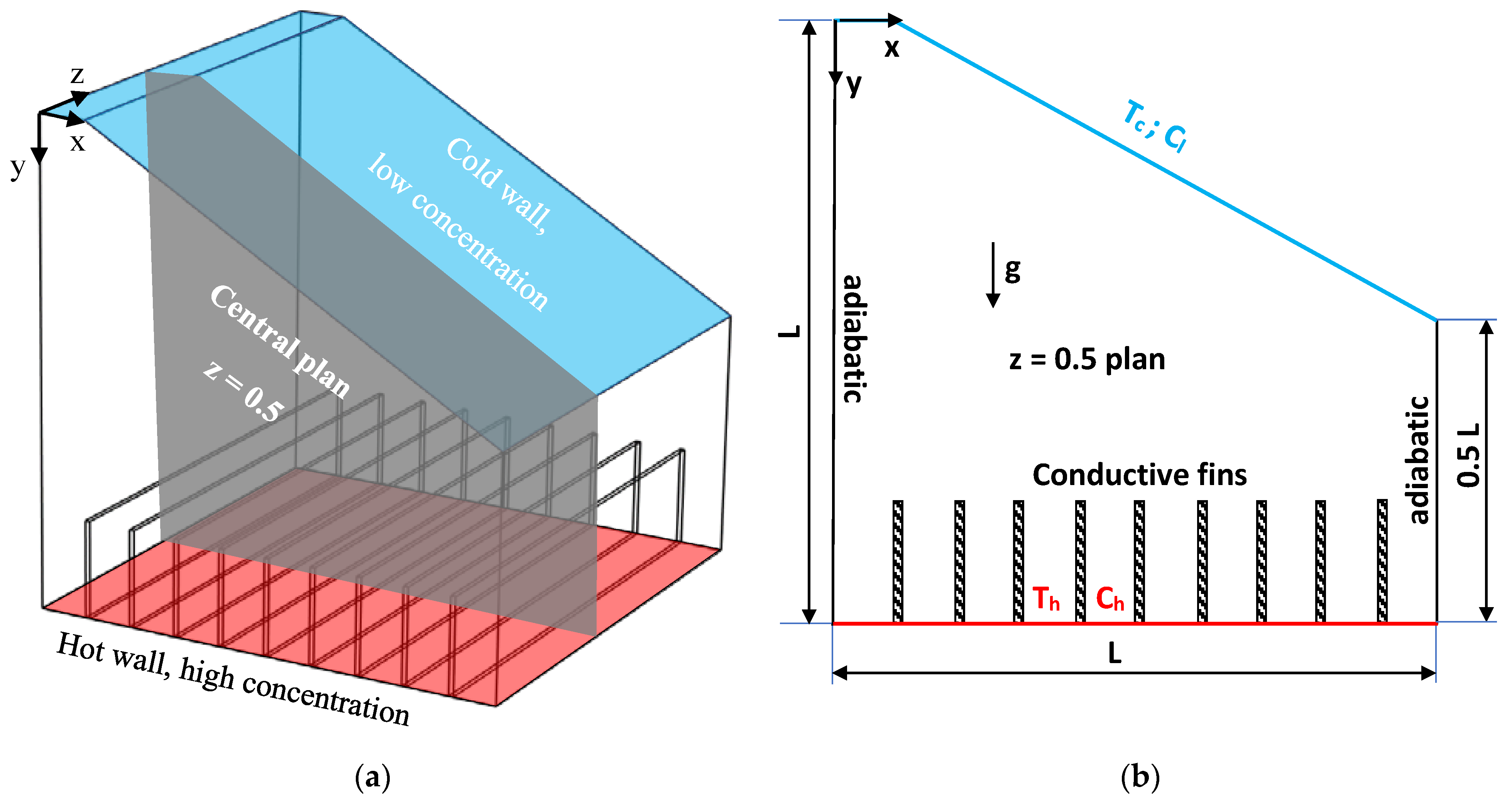
The studied configuration (Figure 1) consists of a 3D trapezoidal solar still filled with air-vapor mixture (Pr = 0.7 and Le = 0.85). The bottom wall is maintained at hot temperature (T_h) and high concentration (C_h), despite the top walls are kept at cold temperature (T_c) and low concentration (C_l). Practically the evaporation of water occurs at the bottom hot wall and the condensation at the top cold wall. The bottom wall of the cavity is equipped with nine conductive fins. The width and height of the fin are 0.01 L and 0.2 L, respectively.

3. Mathematical Formulation

The double diffusive laminar natural convection of a Newtonian and incompressible vapour mixture under the Boussinesq approximation is considered. Neglecting the radiation and Soret and Dufour effects, the dimensional equations governing the studied configuration are expressed as follows:

Continuity:

$$\nabla {\overrightarrow{V}}^{\prime }=0$$

(1)

Momentum:

$$\frac{\partial {\overrightarrow{V}}^{\prime }}{\partial t^{\prime }}+\left(\overrightarrow{V}\times {}^{\prime }\overrightarrow{\nabla }\right){\overrightarrow{V}}^{\prime }=-\frac{1}{{\rho }_0}\overrightarrow{\nabla }{P}^{\prime }+\nu \Delta {\overrightarrow{V}}^{\prime }+\left[1-{\beta }_T\left(T^{\prime }-T_0\right)-{\beta }_C\left(C^{\prime }-C_0\right)\right]\overrightarrow{g}$$

(2)

Energy:

$$\begin{array}{l}\frac{\partial T^{\prime }}{\partial t^{\prime }}+{\overrightarrow{V}}^{\prime }\times \nabla T^{\prime }=\alpha \Delta T^{\prime } \mathrm{in} \mathrm{the} \mathrm{fluid} \mathrm{domain}\\ \frac{\partial T^{\prime }}{\partial t^{\prime }}={\alpha }_{fin}·\Delta T^{\prime } \mathrm{in} \mathrm{the} \mathrm{solid} \mathrm{domains} (\mathrm{fins})\end{array}$$

(3)

Mass:

$$\frac{\partial C^{\prime }}{\partial t^{\prime }}+{\overrightarrow{V}}^{\prime }\times \nabla C^{\prime }=D\Delta C^{\prime }.$$

(4)

One of the most important problems encountered when solving the Navier–Stocks equations is the treatment of the pressure gradient terms, especially in 3D configurations [23]. The vector potential-vorticity formalism is an interesting mathematical transformation allowing to overcome this problem by applying the rotational operation to the momentum equation and thus eliminates the pressure gradient terms.

The vector potential and vorticity are defined by ${\overrightarrow{V}}^{\prime }=\overrightarrow{\nabla }\times {\overrightarrow{\psi }}^{\prime }$ and ${\overrightarrow{\omega }}^{\prime }=\overrightarrow{\nabla }\times {\overrightarrow{V}}^{\prime }$, respectively.

In addition, to get the dimensionless equations the following variables are introduced:

$$\begin{gathered} \left(x,y,z\right)=\left(x^{\prime },y^{\prime },z^{\prime }\right)/L; \omega =\frac{\alpha {\omega }^{\prime }}{L^2}; t=\alpha t^{\prime }/L^2; \psi ={\psi }^{\prime }/\alpha ; \\ (V_1, V_2, V_3)=\left({V^{\prime }}_1, {V^{\prime }}_2, {V^{\prime }}_3\right)·L/\alpha ; \end{gathered}$$

$$T=\frac{T^{\prime }-{T^{\prime }}_c}{{T^{\prime }}_H-{T^{\prime }}_c} \mathrm{and} C=\frac{C^{\prime }-{C^{\prime }}_l}{{C^{\prime }}_h-{C^{\prime }}_l}$$

Thus, by applying the 3D vector potential-vorticity formalism and using the above-mentioned dimensionless variables the set of governing equations becomes:

$$-\overrightarrow{\omega }={\nabla }^2\overrightarrow{\psi }$$

(5)

$$\nabla \overrightarrow{V}=0$$

(6)

$$\begin{array}{ll}\frac{\partial \overrightarrow{\omega }}{\partial t}+\left(\overrightarrow{V}\times \overrightarrow{\nabla }\right)\overrightarrow{\omega }& -\left(\overrightarrow{\omega }\times \overrightarrow{\nabla }\right)\overrightarrow{V}\\ & =Pr\times {\nabla }^2\overrightarrow{\omega }+RaPr\left[\frac{\partial T}{\partial z},0,-\frac{\partial T}{\partial x}\right]-RaPrN\left[\frac{\partial C}{\partial z},0,-\frac{\partial C}{\partial x}\right]\end{array}$$

(7)

$$\begin{gathered} \frac{\partial T}{\partial t}+\overrightarrow{V}\times \nabla T={\nabla }^{2}T \mathrm{in} \mathrm{the} \mathrm{fluid} \mathrm{domain} \\ \frac{\partial T}{\partial t}=\frac{{\alpha }_{fin}}{\alpha }{\nabla }^{2}T \mathrm{in} \mathrm{the} \mathrm{solid} \mathrm{domain} \end{gathered}$$

(8)

$$\frac{\partial C}{\partial t}+\overrightarrow{V}\times \overrightarrow{\nabla }C=\frac{1}{Le}{\overrightarrow{\nabla }}^{2}C.$$

(9)

where:

• $N=\frac{{\beta }_C\left({C^{\prime }}_h-{C^{\prime }}_l\right)}{{\beta }_T\left({T^{\prime }}_H-{T^{\prime }}_c\right)}$ is the buoyancy ratio (Solutal to thermal);
• $Ra=\frac{g{\beta }_T\left({T^{\prime }}_h-{T^{\prime }}_c\right)L^3}{\nu \alpha }$ is the Rayleigh number;
• $\mathit{Pr}=\frac{\nu }{\alpha }$ is the Prandtl number;
• and $Le=\frac{\alpha }{D}$ is the Lewis number.

The temperature continuity at the fins/air-vapor mixture interface is ensured by applying the following expression:

${\left(\frac{\partial T}{\partial n}\right)}_f=Rc.{\left(\frac{\partial T}{\partial n}\right)}_{fin}$, with $Rc=\frac{k_{fin}}{k}$ is conductivity ratio

The local Nusselt and Sherwood numbers at the top cold wall are expressed as:

$$Nu=\left.\frac{\partial T}{\partial n}\right| \mathrm{and} Sh=\left.\frac{\partial C}{\partial n}\right|$$

and the average values of Nusselt and Sherwood numbers are evaluated by:

$$N{u}_{av}=\frac{1}{s}{{\displaystyle \int }}_0^s{{\displaystyle \int }}_0^{1}Nu.\partial \tau .\partial z \mathrm{and} S{h}_{av}=\frac{1}{s}{{\displaystyle \int }}_0^s{{\displaystyle \int }}_0^{1}Sh.\partial \tau .\partial z$$

The applied boundary conditions are:

• $T=1$ at the bottom wall, $T=0$ at the top walls, and $\frac{\partial T}{\partial n}=0$ at the lateral walls.
• $C=1$ at the bottom wall, $C=0$ at the top walls, and $\frac{\partial C}{\partial n}=0$ at the lateral walls and fins surfaces.
• $\overrightarrow{V}=\overrightarrow{0}$ at all the internal and external walls.

4. Numerical Method

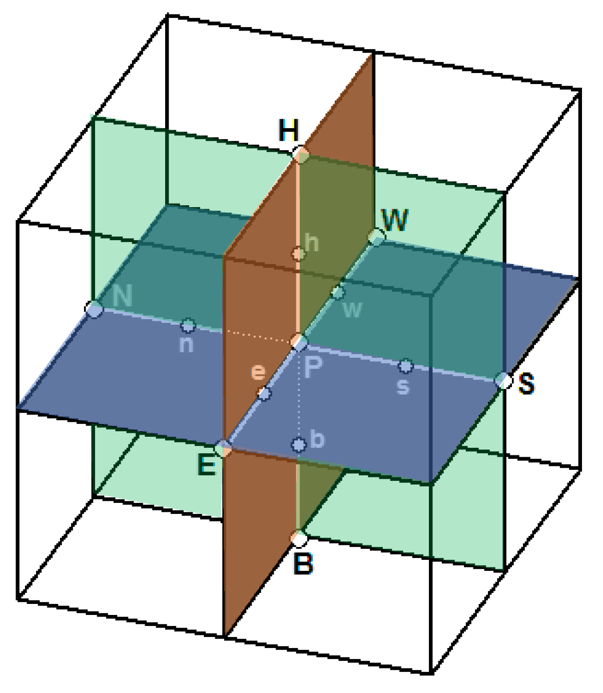
The governing Equations (5)–(8) are solved using the finite volume method (FVM) [24]. The FVM consists of transforming the computational domain to control volumes. In our case these control volumes are cubic, because of the uniform grid size in all the directions (Figure 2). The generated nodes are the points where the algebraic equations are obtained by integration, and all the variables are evaluated iteratively. The number of nodes in all direction is denoted by ‘n’ and the uniform space steps in the directions x, y and z are denoted by Δx, Δy and Δz, respectively.

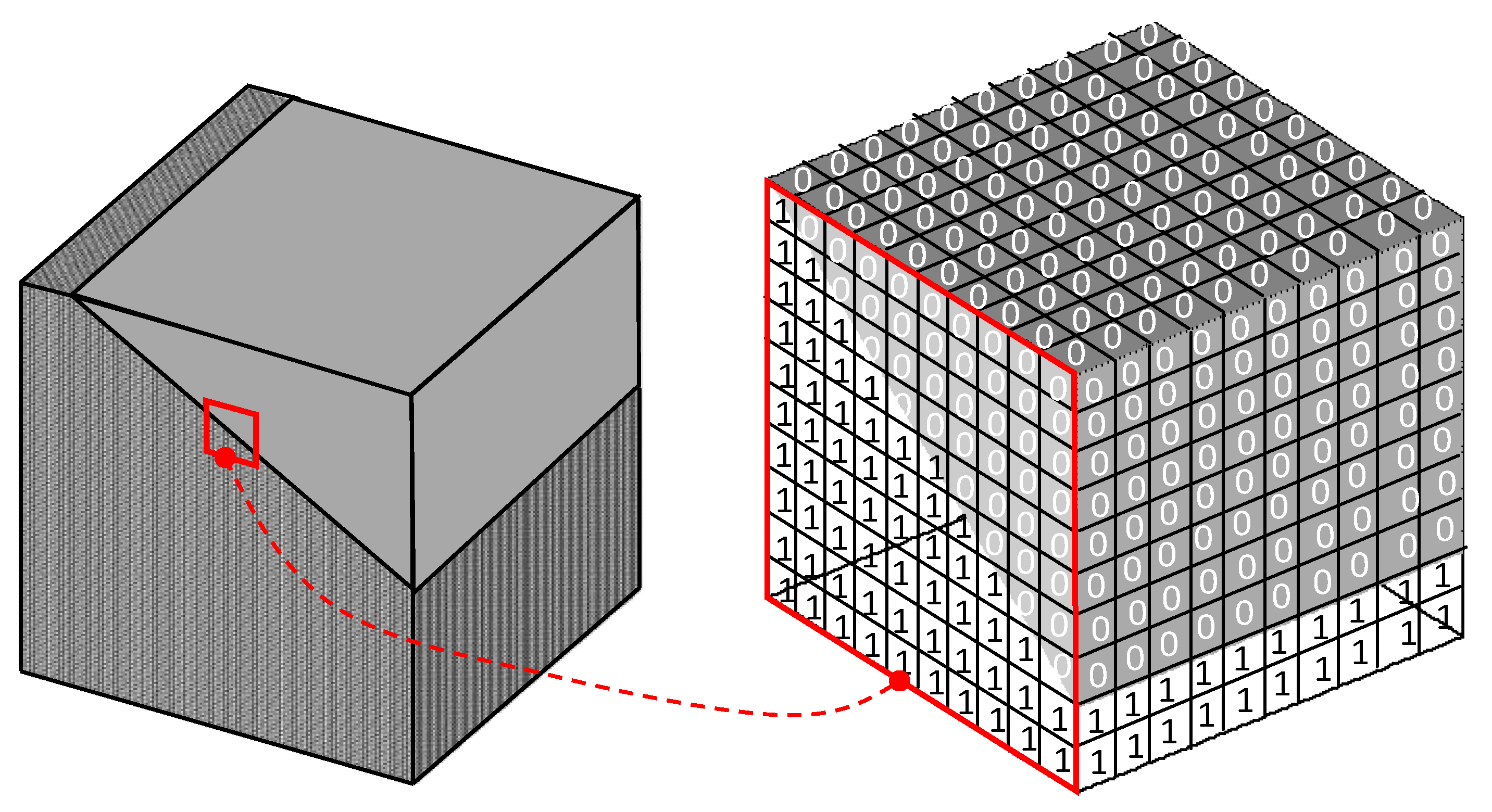
The problem of the present study is that the studied configuration is irregular due to the existence of the top inclined wall where the vapor will condensate. To overcome this issue, the blocked-off-region method is used [24]. The principle of this technique is based on subdividing the domain to active (‘1’) and inactive (‘0’) zones (Figure 3). In this technique, it is necessary to use finer mesh as much as possible to approximate the real boundary separating the active and inactive zone with more accuracy. Even though in this technique a number of fictive nodes are used, it does not require more computational time because all the variables are defined as known in the inactive zones that can be considered in the present case as immobile (V = 0) and isothermal solid (T = T_c).

The generalised form of the governing equations can be presented as:

$$\frac{\partial \mathsf{\Omega }}{\partial t}+\frac{\partial }{\partial x}\left(V_x·\mathsf{\Omega }-\mathsf{\Gamma }\frac{\partial \mathsf{\Omega }}{\partial x}\right)+\frac{\partial }{\partial y}\left(V_y·\mathsf{\Omega }-\mathsf{\Gamma }\frac{\partial \mathsf{\Omega }}{\partial y}\right)+\frac{\partial }{\partial z}\left(V_z·\mathsf{\Omega }-\mathsf{\Gamma }\frac{\partial \mathsf{\Omega }}{\partial z}\right)=\mathrm{S}$$

The total thermal and solutal convective fluxes in the three directions x, y and z are defined as $F{l}_x=V_x\mathsf{\Omega }-\mathsf{\Gamma }\frac{\partial \mathsf{\Omega }}{\partial x}$, $F{l}_y=V_y\mathsf{\Omega }-\mathsf{\Gamma }\frac{\partial \mathsf{\Omega }}{\partial Y}$ and $F{L}_z=V_z\mathsf{\Omega }-\mathsf{\Gamma }\frac{\partial \mathsf{\Omega }}{\partial Z}$, respectively. Thus, the general equation can be simplified to the following form:

$$\frac{\partial \mathsf{\Omega }}{\partial t}+\frac{\partial F{L}_x}{\partial x}+\frac{\partial F{L}_y}{\partial y}+\frac{\partial F{L}_z}{\partial z}=\mathrm{S}$$

The integral form of this equation on the control volume gives:

$$\begin{gathered} \left({\mathsf{\Omega }}_p-{\mathsf{\Omega }}_p^{*}\right)\Delta x\Delta y\Delta z+\left(F{L}_{xe}-F{L}_{xw}\right)\Delta y\Delta z\Delta t+\left(F{L}_{yn}-F{L}_{ys}\right)\Delta x\Delta z\Delta t \\ +\left(F{L}_{zh}-F{L}_{zb}\right)\Delta x\Delta y\Delta t=\overline{S}\Delta x\Delta y\Delta z\Delta t \end{gathered}$$

The superscript “*” denotes the precedent temporal iteration.

Considering:

$$F{L}_e=F{L}_{xe}\Delta y\Delta z F{L}_w=F{L}_{xw}\Delta y\Delta z F{L}_n=F{L}_{yn}\Delta x\Delta z,L_s=F{L}_{ys}\Delta x\Delta z$$

$$F{L}_h=F{L}_{zh}\Delta x\Delta y \mathrm{and} F{L}_b=L_{zb}\Delta x\Delta y$$

and dividing by Δt,

The general discretised equation becomes:

$$\left({\mathsf{\Omega }}_p-{\mathsf{\Omega }}_p^{*}\right)\frac{\Delta x\Delta y\Delta z}{\Delta t}+\left(F{L}_e-F{L}_w\right)+\left(F{L}_n-F{L}_s\right)+\left(F{L}_h-F{L}_b\right)=\overline{S}\Delta x\Delta y\Delta z$$

where:

$$\overline{S}=S_c+S_p{\mathsf{\Omega }}_p$$

The integration of the dimensionless continuity of equation on the control volume, gives:

$$\left(V_{xe}\Delta y\Delta z-V_{xw}\Delta y\Delta z\right)+\left(V_{yn}\Delta x\Delta z-V_{ys}\Delta x\Delta z\right)+\left(V_{zh}\Delta x\Delta y-V_{zb}\Delta x\Delta y\right)=0$$

The mass flow rates crossing the six faces of the control volume are:

$$M_e=V_{xe}\Delta y\Delta z \mathrm{and} M_w=V_{xw}\Delta y\Delta z; F_n=V_{yn}\Delta x\Delta z \mathrm{and} M_s=V_{ys}\Delta x\Delta z; M_h=V_{zs}\Delta x\Delta y \mathrm{and} M_b=V_{zb}\Delta x\Delta y$$

Thus, the discretised continuity equation is simplified as:

$$\left(M_e-M_w\right)+\left(M_n-M_s\right)+\left(M_h-M_b\right)=0$$

By multiplying this equation by ${\mathsf{\Omega }}_p$ and subtracting it from the general discretised equation, we get:

$$\begin{array}{ll}{\mathsf{\Omega }}_p\left(\frac{\Delta x\Delta y\Delta z}{\Delta t}-S_p\Delta x\Delta y\Delta z\right)& +\left(F{L}_e-M_e{\mathsf{\Phi }}_p\right)-\left(F{L}_w-M_w{\mathsf{\Omega }}_p\right)\\ & +\left(F{L}_n-M_n{\mathsf{\Omega }}_p\right)-\left(F{L}_s-M_s{\mathsf{\Omega }}_p\right)+\left(F{L}_h-M_h{\mathsf{\Omega }}_p\right)\\ & -\left(F{L}_b-M_b{\mathsf{\Omega }}_p\right)=\left(S_c\Delta x\Delta y\Delta z+{\mathsf{\Omega }}_p^{*}\frac{\Delta x\Delta y\Delta z}{\Delta t}\right)\end{array}$$

According to [24]: $\left(F{L}_n-M_n{\mathsf{\Omega }}_p\right)=a_N\left({\mathsf{\Omega }}_p-{\mathsf{\Omega }}_N\right)$, $\left(F{L}_s-M_s{\mathsf{\Omega }}_p\right)=a_S\left({\mathsf{\Omega }}_S-{\mathsf{\Omega }}_p\right)$, $\left(F{L}_e-M_e{\mathsf{\Omega }}_p\right)=a_E\left({\mathsf{\Omega }}_p-{\mathsf{\Omega }}_E\right)$, $\left(F{L}_w-M_w{\mathsf{\Omega }}_p\right)=a_W\left({\mathsf{\Omega }}_W-{\mathsf{\Omega }}_p\right)$, $\left(F{L}_h-M_h{\mathsf{\Omega }}_p\right)=a_H\left({\mathsf{\Omega }}_p-{\mathsf{\Omega }}_H\right)$, $\left(F{L}_b-M_b{\mathsf{\Omega }}_p\right)=a_B\left({\mathsf{\Omega }}_B-{\mathsf{\Omega }}_p\right)$.

The discretised general equation becomes:

$$a_p{\mathsf{\Omega }}_p=a_E{\mathsf{\Omega }}_E+a_W{\mathsf{\Omega }}_W+a_N{\mathsf{\Omega }}_N+a_S{\mathsf{\Omega }}_S+a_H{\mathsf{\Omega }}_H+a_B{\mathsf{\Omega }}_B+b_p$$

With:

$$a_p=a_E+a_W+a_N+a_S+a_H+a_B+\frac{\Delta x\Delta y\Delta z}{\Delta t}-S_p\Delta x\Delta y\Delta z \mathrm{and} b_p=S_c\Delta x\Delta y\Delta z+{\mathsf{\Omega }}_p^{*}\frac{\Delta x\Delta y\Delta z}{\Delta t}$$

The set of discretised governing equations is written by replacing Ω by the variables and by using the central-difference scheme to treat the convective terms:

• T

  $$a_p{T}_p=a_E{T}_E+a_W{T}_W+a_N{T}_N+a_S{T}_S+a_H{T}_H+a_B{T}_B+b_p \mathrm{with} b_p=T_p^{°}\frac{\Delta x\Delta y\Delta z}{\Delta t}$$
• C

  $$a_p{C}_p=a_E{C}_E+a_W{C}_W+a_N{C}_N+a_S{C}_S+a_H{C}_H+a_B{C}_B+b_p \mathrm{with} b_p=C_p^{°}\frac{\Delta x\Delta y\Delta z}{\Delta t}$$
• ${\omega }_x$

  $$a_p{\omega }_{xp}=a_E{\omega }_{xE}+a_W{\omega }_{xW}+a_N{\omega }_{xN}+a_S{\omega }_{xS}+a_H{\omega }_{xH}+a_B{\omega }_{xB}+b_p$$

With

$$\begin{array}{ll}{b}_p={\omega }_{xp}^{°}\frac{\Delta x\Delta y\Delta z}{\Delta t}& +{\omega }_{xp}\left(\frac{V_{xE}-V_{xw}}{2}\right)\Delta y\Delta z+{\omega }_{yp}\left(\frac{V_{xS}-V_{xN}}{2}\right)\Delta x\Delta z\\ & +{\omega }_{zp}\left(\frac{V_{xH}-V_{xB}}{2}\right)\Delta x\Delta y+Ra\mathit{Pr}\left(\frac{T_H-T_B}{2}\right)\Delta x\Delta y\\ & -Ra\mathit{Pr}N\left(\frac{C_H-C_B}{2}\right)\Delta x\Delta y\end{array}$$

• ${\omega }_y$

  $$a_p{\omega }_{xp}=a_E{\omega }_{yE}+a_W{\omega }_{yW}+a_N{\omega }_{yN}+a_S{\omega }_{yS}+a_H{\omega }_{yH}+a_B{\omega }_{yB}+b_p$$

With

$$\begin{array}{ll}{b}_p={\omega }_{yp}^{°}\frac{\Delta x\Delta y\Delta z}{\Delta t}& +{\omega }_{yp}\left(\frac{V_{yE}-V_{yw}}{2}\right)\Delta y\Delta z+{\omega }_{yp}\left(\frac{V_{yS}-V_{yN}}{2}\right)\Delta x\Delta z\\ & +{\omega }_{zp}\left(\frac{V_{yH}-V_{yB}}{2}\right)\Delta x\Delta y\end{array}$$

• ${\omega }_z$

  $$a_p{\omega }_{zp}=a_E{\omega }_{zE}+a_W{\omega }_{zW}+a_N{\omega }_{zN}+a_S{\omega }_{zS}+a_H{\omega }_{zH}+a_B{\omega }_{zB}+b_p$$

With

$$\begin{array}{ll}{b}_p={\omega }_{zp}^{°}\frac{\Delta x\Delta y\Delta z}{\Delta t}& +{\omega }_{zp}\left(\frac{V_{zE}-V_{zw}}{2}\right)\Delta y\Delta z+{\omega }_{zp}\left(\frac{V_{zS}-V_{zN}}{2}\right)\Delta x\Delta z\\ & +{\omega }_{zp}\left(\frac{V_{zH}-V_{zB}}{2}\right)\Delta x\Delta y-Ra\mathit{Pr}\left(\frac{T_E-T_W}{2}\right)\Delta y\Delta z\\ & +Ra\mathit{Pr}N\left(\frac{C_E-C_W}{2}\right)\Delta y\Delta z\end{array}$$

• ${\Psi }_{xp}=\frac{1}{2\left(\frac{1}{\Delta x^2}+\frac{1}{\Delta y^2}+\frac{1}{\Delta z^2}\right)}\left(\frac{{\Psi }_{xE}+{\Psi }_{xW}}{\Delta x^2}+\frac{{\Psi }_{xN}+{\Psi }_{xS}}{\Delta y^2}+\frac{{\Psi }_{xH}+{\Psi }_{xB}}{\Delta z^2}+{\omega }_{xp}\right)$
• $Ple{\Psi }_{yp}=\frac{1}{2\left(\frac{1}{\Delta x^2}+\frac{1}{\Delta y^2}+\frac{1}{\Delta z^2}\right)}\left(\frac{{\Psi }_{yE}+{\Psi }_{yW}}{\Delta x^2}+\frac{{\Psi }_{yN}+{\Psi }_{yS}}{\Delta y^2}+\frac{{\Psi }_{yH}+{\Psi }_{yB}}{\Delta z^2}+{\omega }_{yp}\right)$
• ${\Psi }_{zp}=\frac{1}{2\left(\frac{1}{\Delta x^2}+\frac{1}{\Delta y^2}+\frac{1}{\Delta z^2}\right)}\left(\frac{{\Psi }_{zE}+{\Psi }_{zW}}{\Delta x^2}+\frac{{\Psi }_{zN}+{\Psi }_{zS}}{\Delta y^2}+\frac{{\Psi }_{zH}+{\Psi }_{zB}}{\Delta z^2}+{\omega }_{zp}\right)$

The described governing equations are discretised via the control volume finite difference method based on the central difference scheme for the convective terms and the implicit procedure for temporal derivative, then a numerical code is developed using Fortran language. To accelerate the convergence of the solution, the successive relaxation technique is used, and the convergence criterion is set as $\frac{max\left|{\mathsf{\Omega }}^m-{\mathsf{\Omega }}^{m-1}\right|}{max\left|{\mathsf{\Omega }}^m\right|}\le {10}^{-5}$ with ‘m’ denoting the temporal iteration.

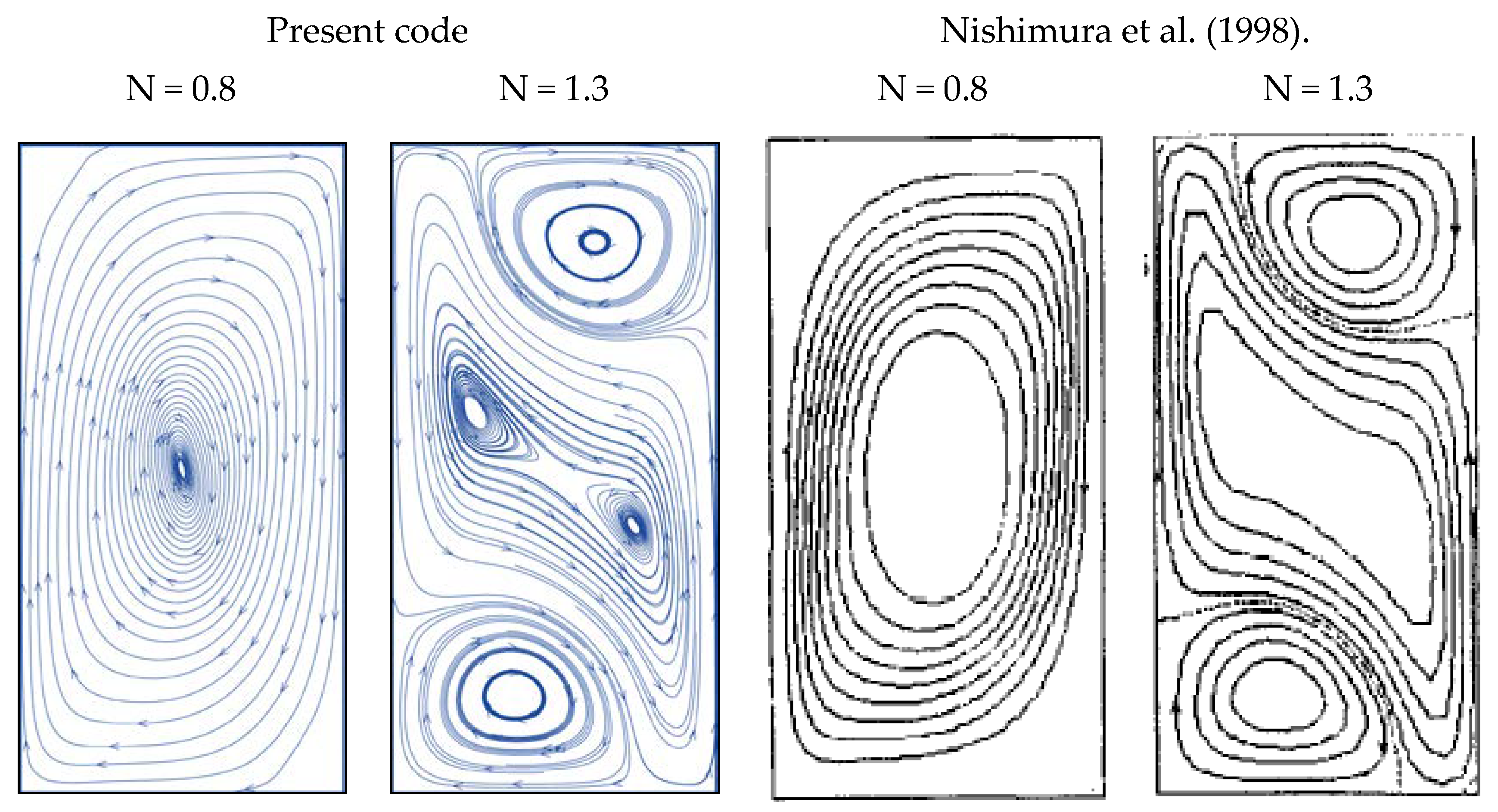
5. Code Verification and Grid Sensitivity Test

To check the validity of the numerical code, a comparison with the findings of Nishimura et al. [25] who studied the double diffusive convection in rectangular cavities, is performed. The comparison of the flow structures presented in Figure 4 shows a good adequacy between the results. It is just to be noted that the streamlines in our case are not closed and looks like vortexes caused by the 3D character that causes a transversal flow.

The mesh sensitivity test (

Table 1. Mesh sensitivity test.

Mesh	Nuav	Percentage Increase	Incremental Increase
903	1.6148	-	-
1103	1.6554	2.5142	-
1303	1.7086	5.8087	3.2137 (%)
1503	1.7123	6.0378	0.2165 (%)

) is performed for Ra = 10⁵, N = −2 and R_c = 100. As presented in

Table 2. Optimised solution.

Solution	N	Ra	Rc	Shav Fit	Nuav Fit	Composite Desirability
1	0	105	100	2.1557	3.9102	1

, four grids have been considered. It is to be mentioned that the number of grids is relatively high to ensure a good approximation of the inclined boundary wall. Nu_av is considered as the sensitive variable and the comparison between the meshes 130³ and 150³ shows that the difference is about 21%. Thus, to get a good accuracy of the results while respecting the computational time, the mesh 130³ was retained for all the numerical executions.

6. Results and Discussion

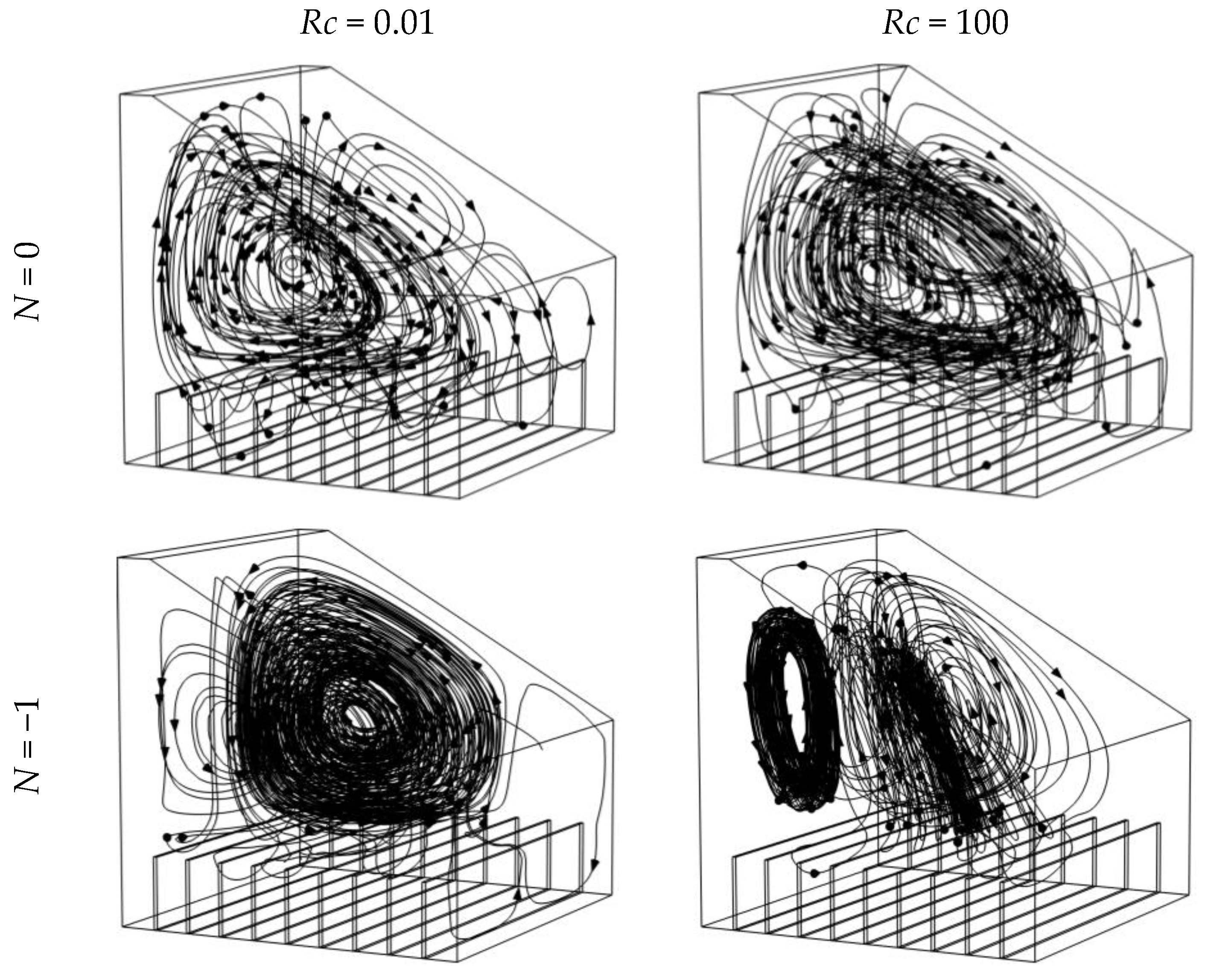
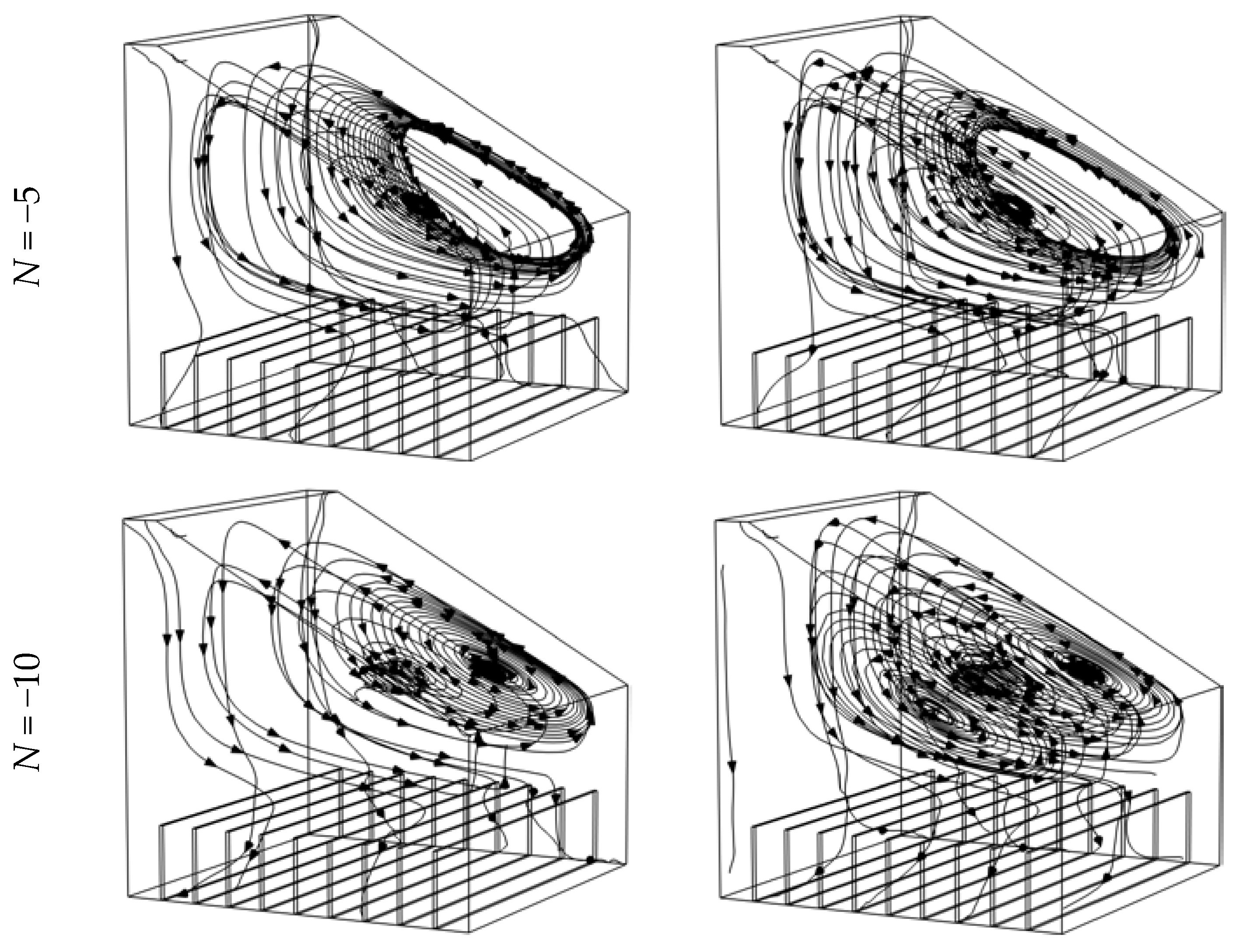
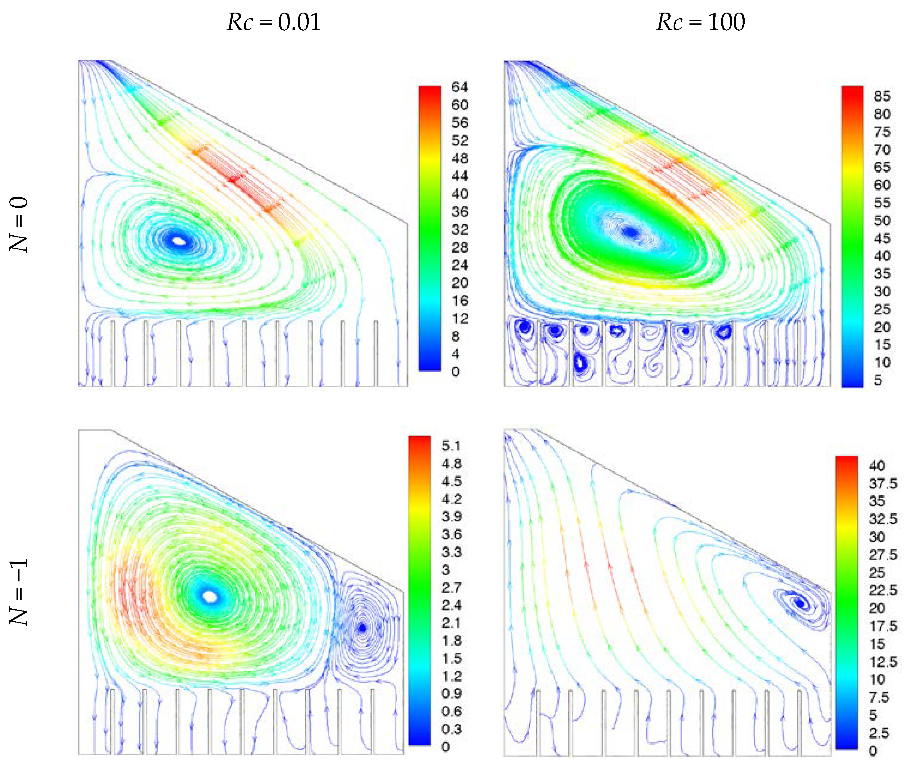
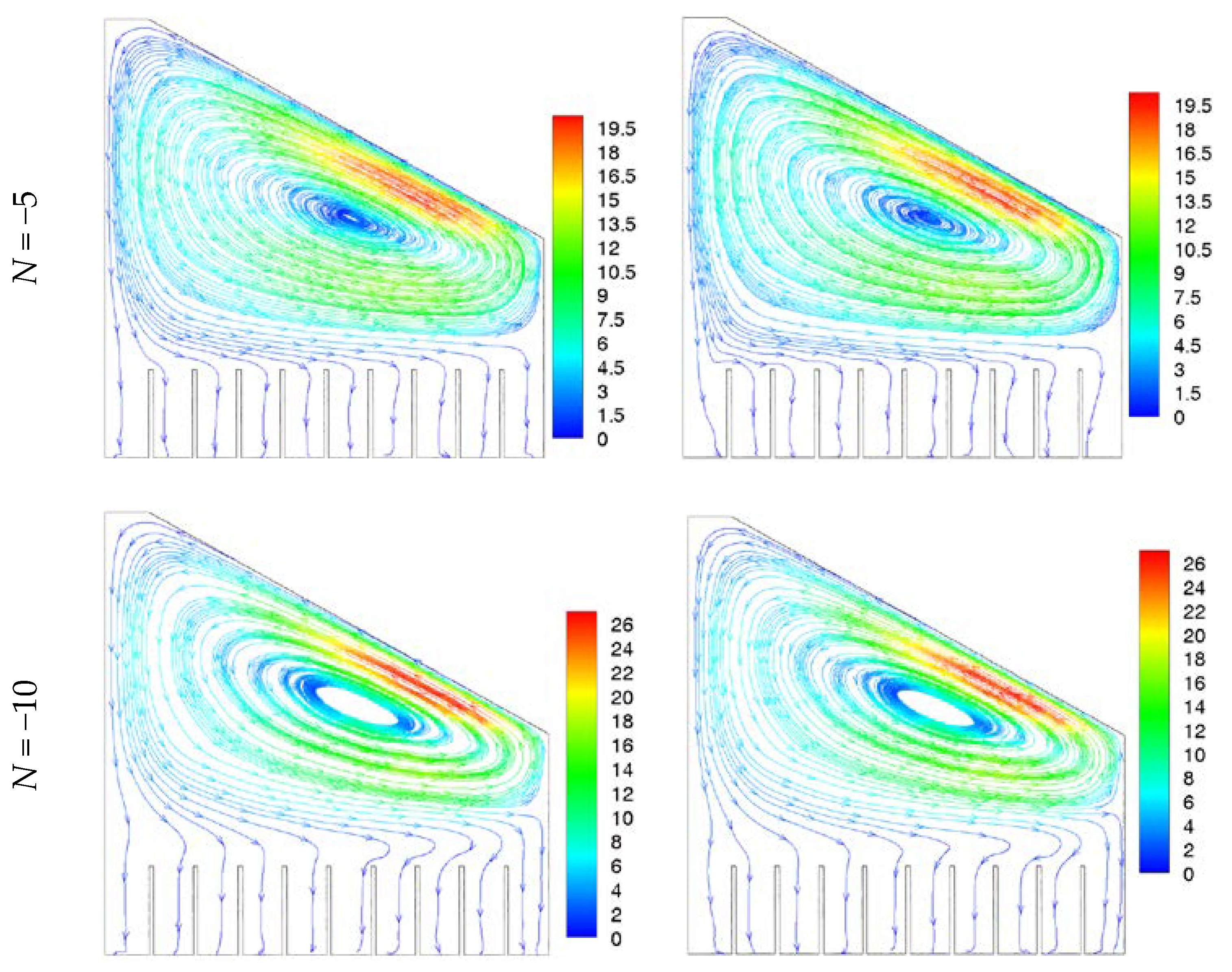
In the present paper the heat and mass transfer in a 3D trapezoidal solar still equipped with conductive fins is studied. The effects of Rayleigh number, the buoyancy ratio and the fins conductivity are investigated. Figure 5 and Figure 6 present the 3D flow structures and the velocity projections at the central plan, respectively for various buoyancy ratios (N) and conductivities ratios (Rc). Compared to the 2D cases, the particles trajectories are not closed, and the flow passes transversally through the cavity from a constant z-plan to another. It is to be mentioned that the considered values of the buoyancy ration are negative, indicating that the thermal and solutal forces are opposing.

For N = 0, the flow direction is clockwise for all the considered Rc, but the flow intensity is more important for higher Rc values due to higher fins conductivity, that allows the heat to be transferred easily to the top region of the cavity. In addition, for Rc = 100, a multitude of secondary flows appear in the regions delimited by the fins.

For N = −1, the flow intensity is reduced due to the equilibrium between the solutal and thermal buoyancy forces. For low Rc values the central main flow is characterised by two counter-rotative vortexes, with a dominance of the solutal vortex that seizes most of the cavity domain. The increase of the heat transfer is proportional to the increase of Rc. Therefore, when heat is transferred to the fluid, the flow becomes non-organised and dominated by the thermal forces.

For both N = −5 and −10, the effect of Rc on the flow structure becomes negligible since the dominance of the solutal forces is marked with one counter-clockwise vortex.

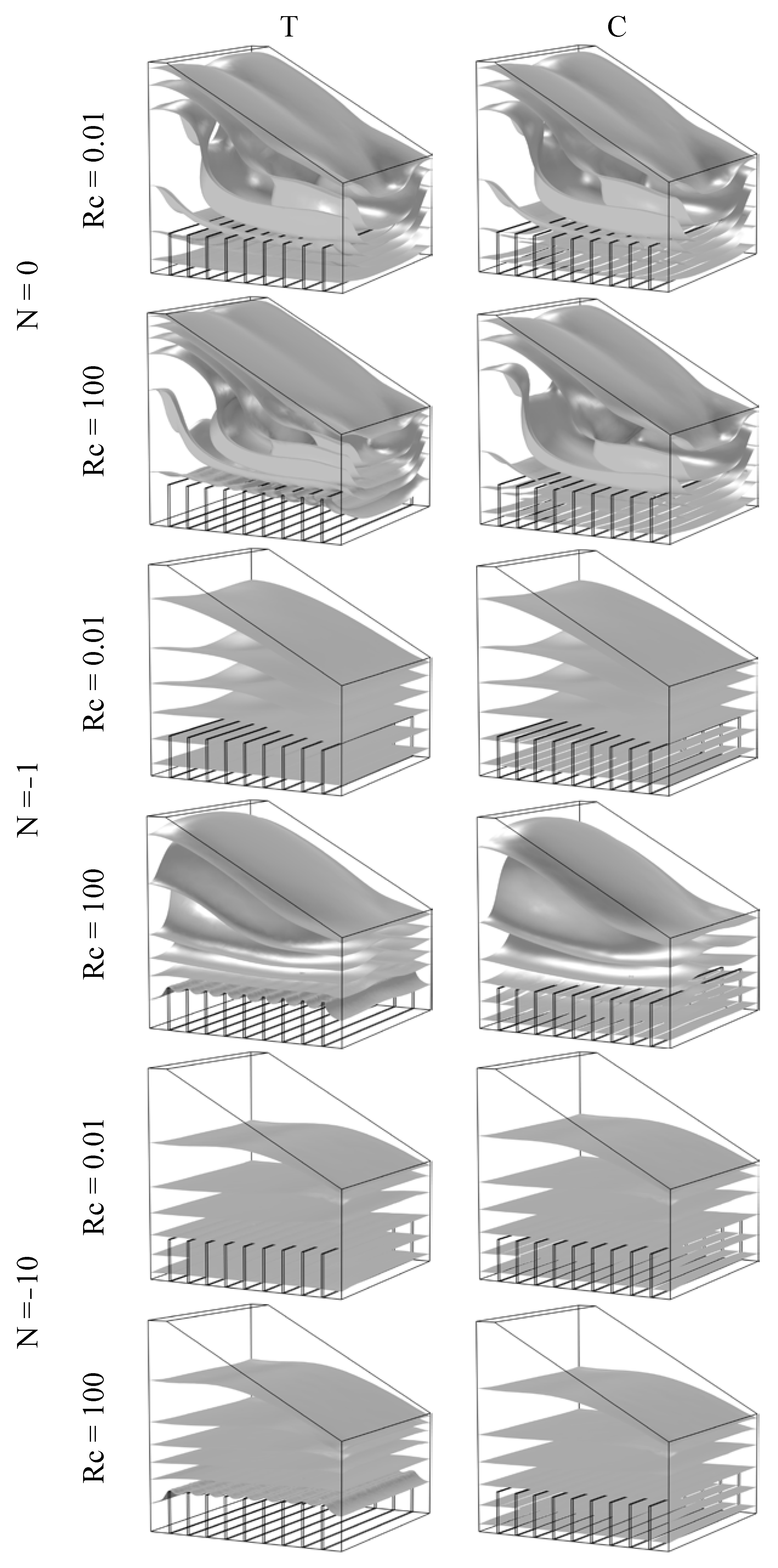
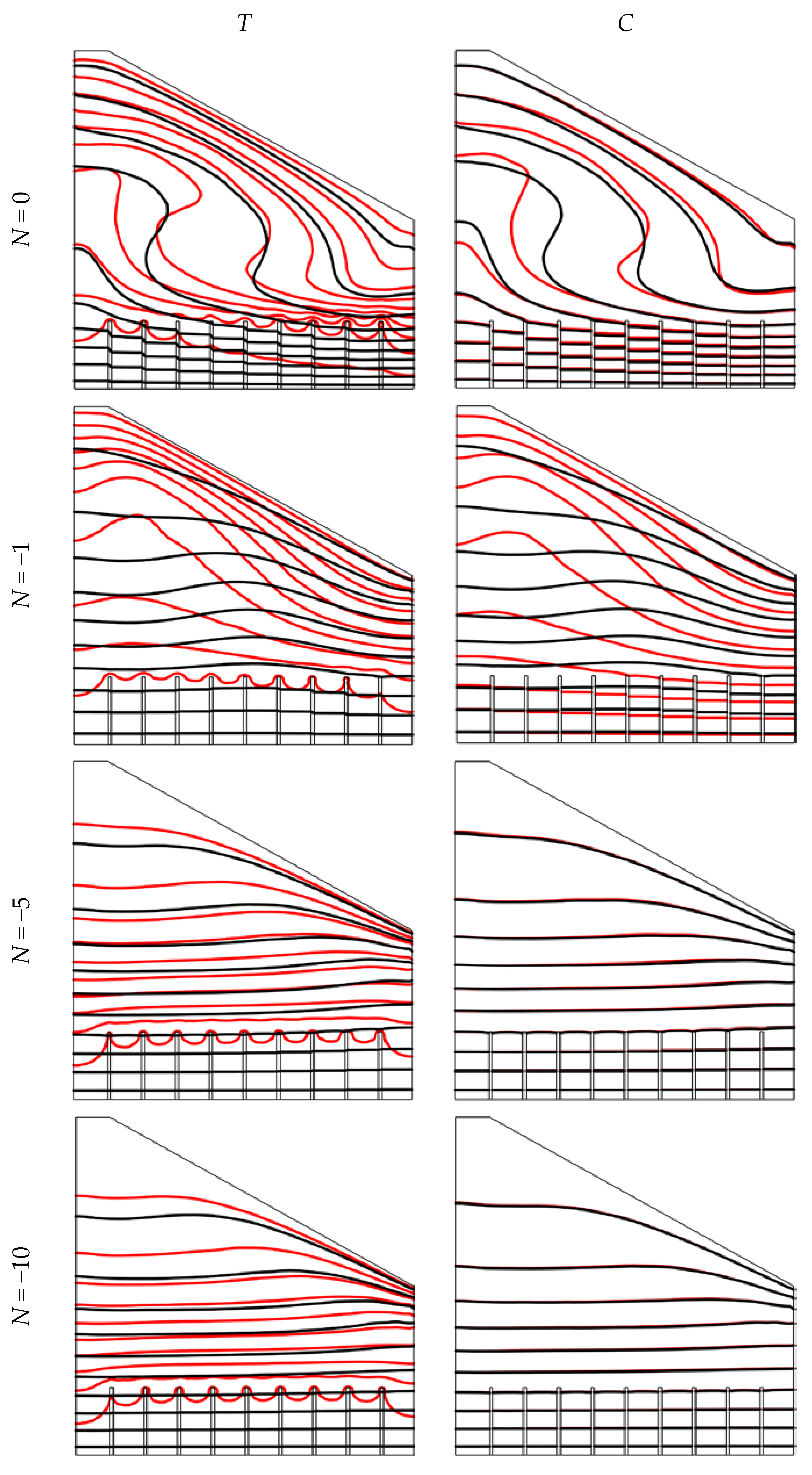
Figure 7 and Figure 8 present the 3D temperature fields and the isotherms and iso-concentration at the central plan, respectively for various buoyancy ratios (N) and conductivity ratios (Rc).

For all the considered cases there is a similarity between the isotherms and the iso-concentration due to the fixed value of Le (=0.85) in the current study which is close to 1. In addition, the effect of the increase of the conductivity of the fins is more pronounced on the isotherms compared to the iso-concentration. In fact, at the central region of the cavity, the distortion of the isotherms and iso-concentrations, caused by the increase of the conductivity of the fins is more important for the isotherms. These distortions indicate the enhancement of the thermal and solutal convections and are more pronounced for N = 0. For N = −1 and low Rc values, the distortions disappear, and the temperature and concentration fields are characterised by a vertical stratification indicating the reduction of buoyancy due to the balanced competitivity between the solutal and thermal forces. For Rc = 0.01, the isotherms are quasi-vertical at the bottom of the cavity due to the low conductivity of the fins. For N = −5 and −10, the effect of Rc on the iso-concentrations is negligible and are quasi-superposed for all Rc values.

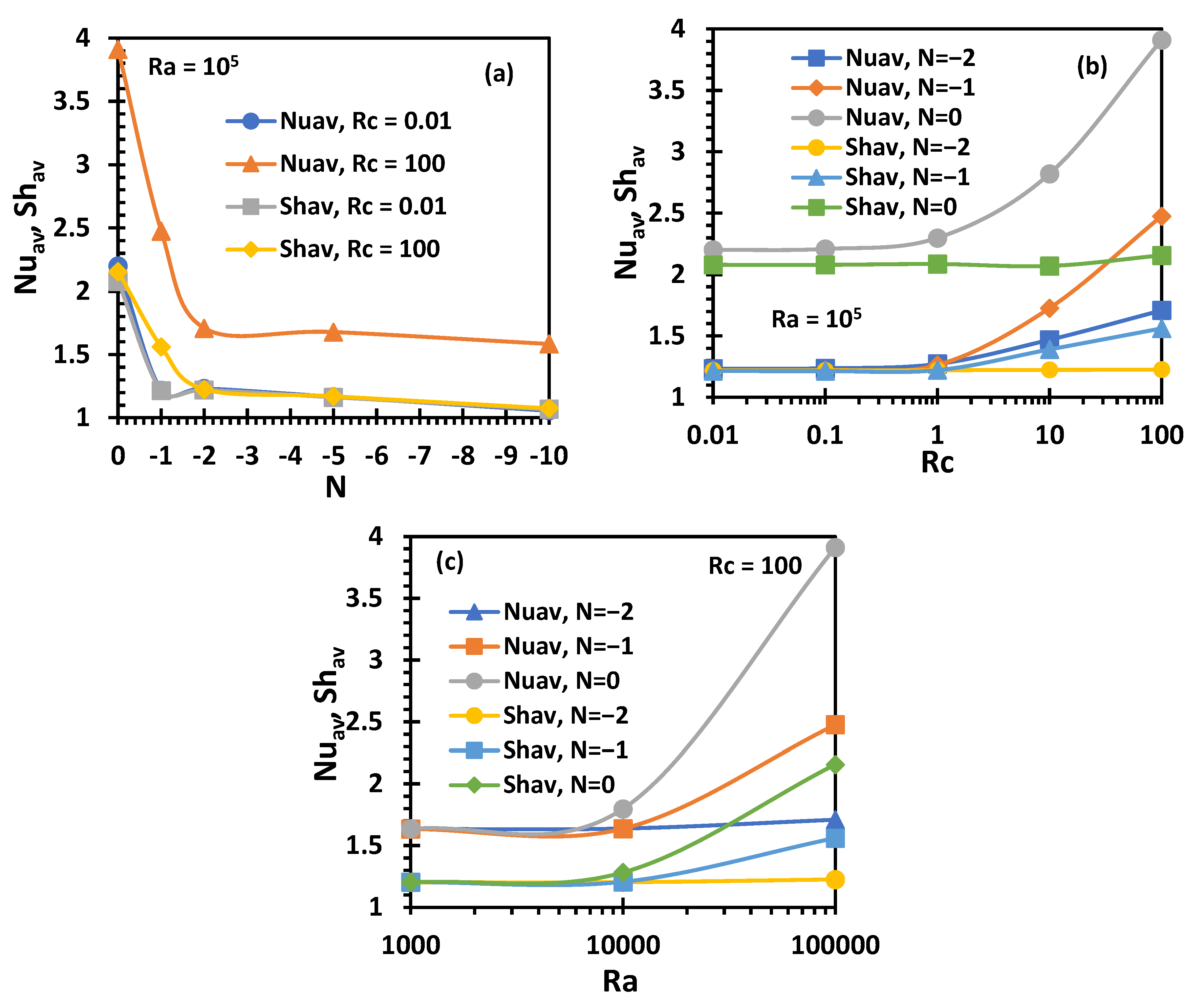
Figure 9a–c, are plotted to explore the effect of the buoyancy ratio, the conductivity ratio and Rayleigh number on the heat and mass transfer. Due the consideration of the opposing thermal and solutal forces, the increase of N (in absolute value) causes a reduction of the heat and mass transfers. In opposition the increase of Rc and Ra causes an enhancement of the heat and mass transfers. It is to be mentioned that the effect of Rc on the mass transfer becomes more and more negligeable when N increases. This is confirmed by the reduction of the concentration gradients close to the cold walls and the apparition the vertical stratification as presented in Figure 8.

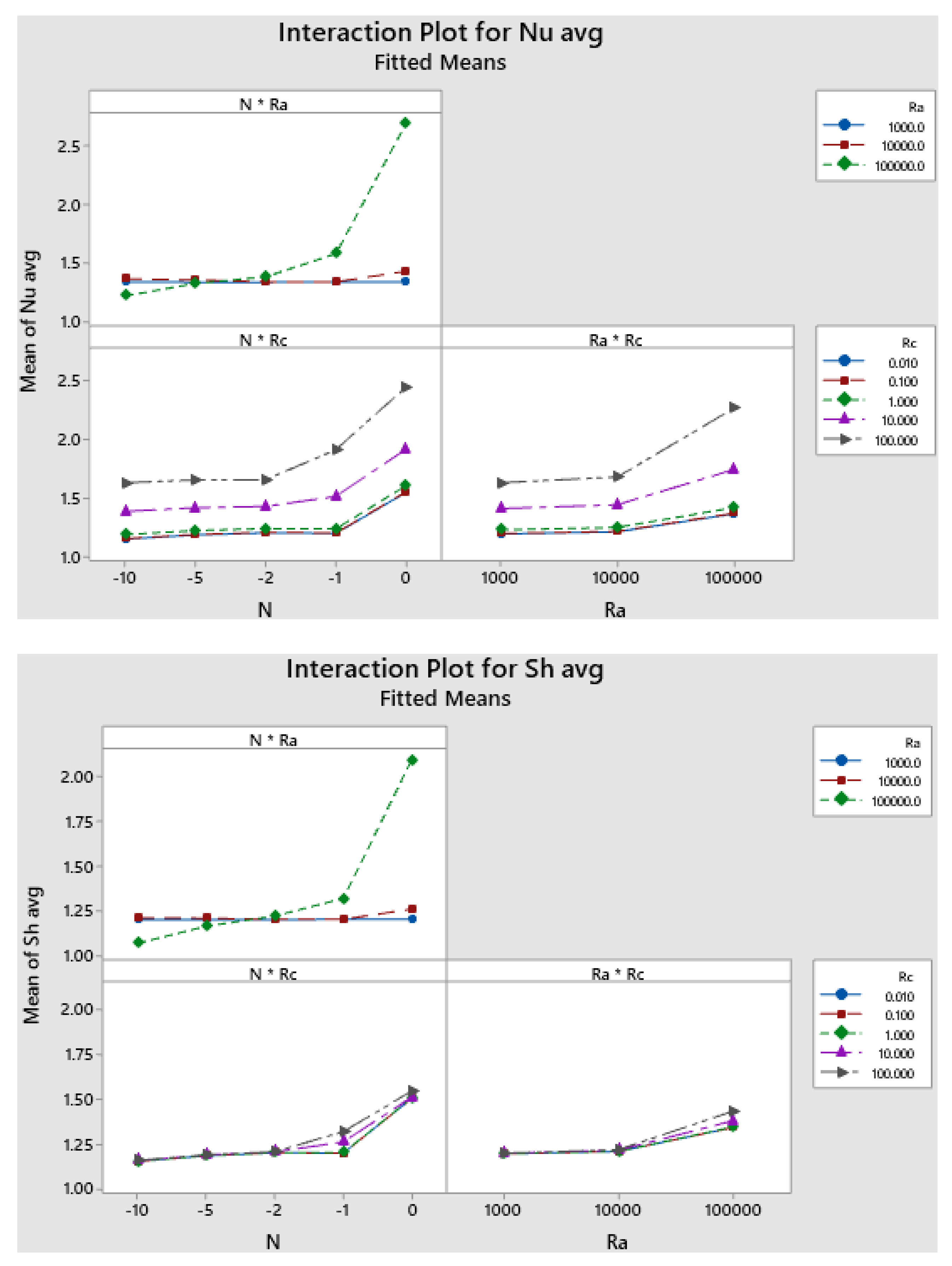
Figure 10 presents the interaction plots between the factors Nu_av = f(N, Ra), Nu_av = f(N, Rc) and Nu_av = f(Ra, Rc).

When N is at its low level, it is clear that the values of Nusselt and Sherwood averages are also at their low levels for all the Rayleigh numbers. By increasing N values, the Nusselt and Sherwood average numbers reach their maximum values. In fact, when Ra = 10⁵, both Shav and Nu_av are at their highest values when N is equal to zero.

From the second and third interaction plots, it is clear that the highest values of Nu_av and Sh_av are localised for the N = 0 and Rc = 100. It is also interesting to add that when Ra = (10³, 10⁴), the values of Nusselt average are almost similar; however, for high value of Ra, the Nu average values increase with the increase of the Rc.

The regression model is carried on and the following equations are determined using Minitab:

Sh_av = 1.2790 + 0.02356·N + 0.000002·Ra + 0.000302·Rc

Nu_av = 1.3330 + 0.0330·N + 0.000003·Ra + 0.005524·Rc

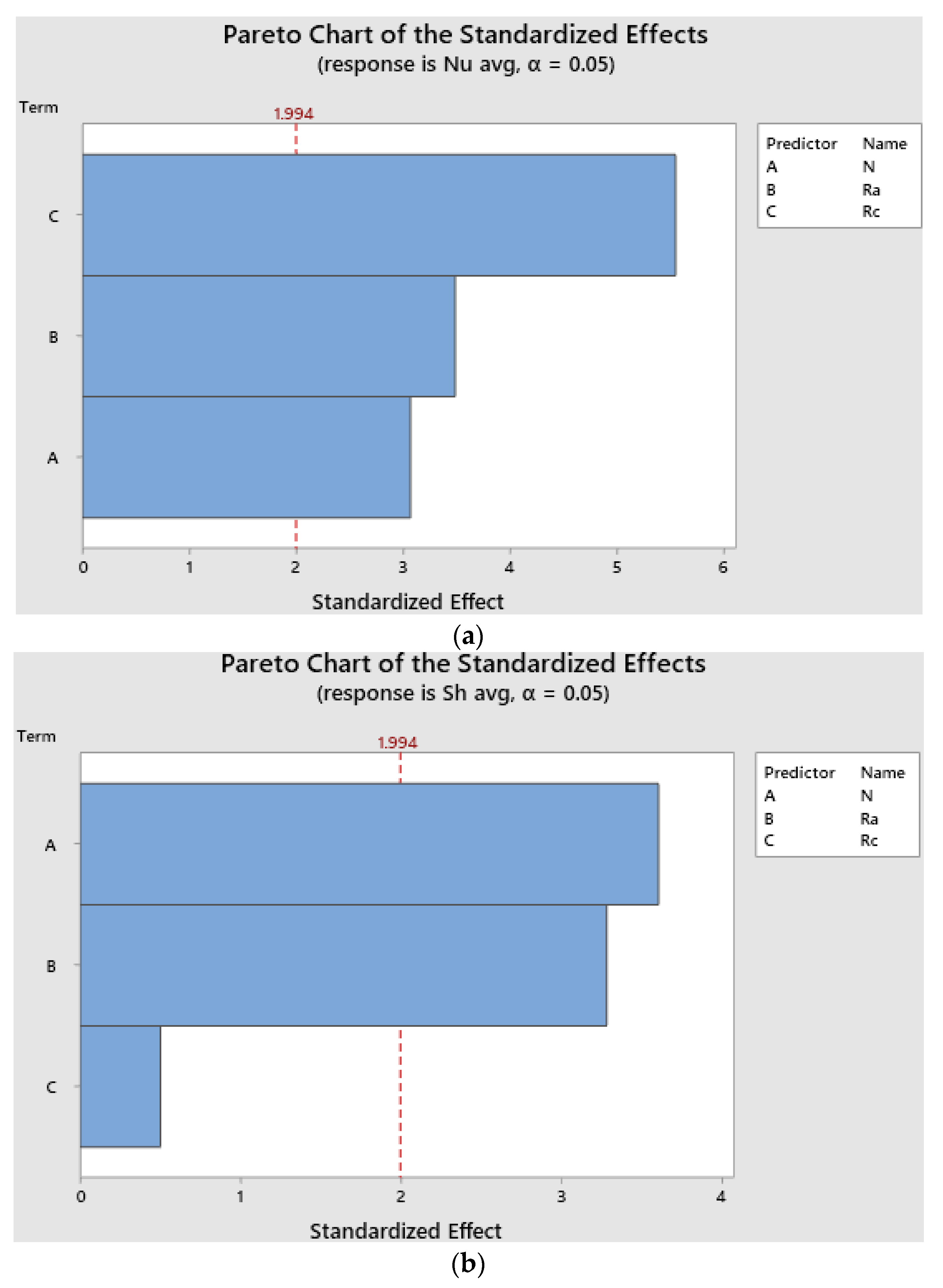
Figure 11 represents the importance of the standardised effects of the different factors of the model i.e., N, Ra, and Rc. It is remarkable that all the factors are important to study the Nu_av effect. However, the Rc factor has a small effect on the average Sherwood number.

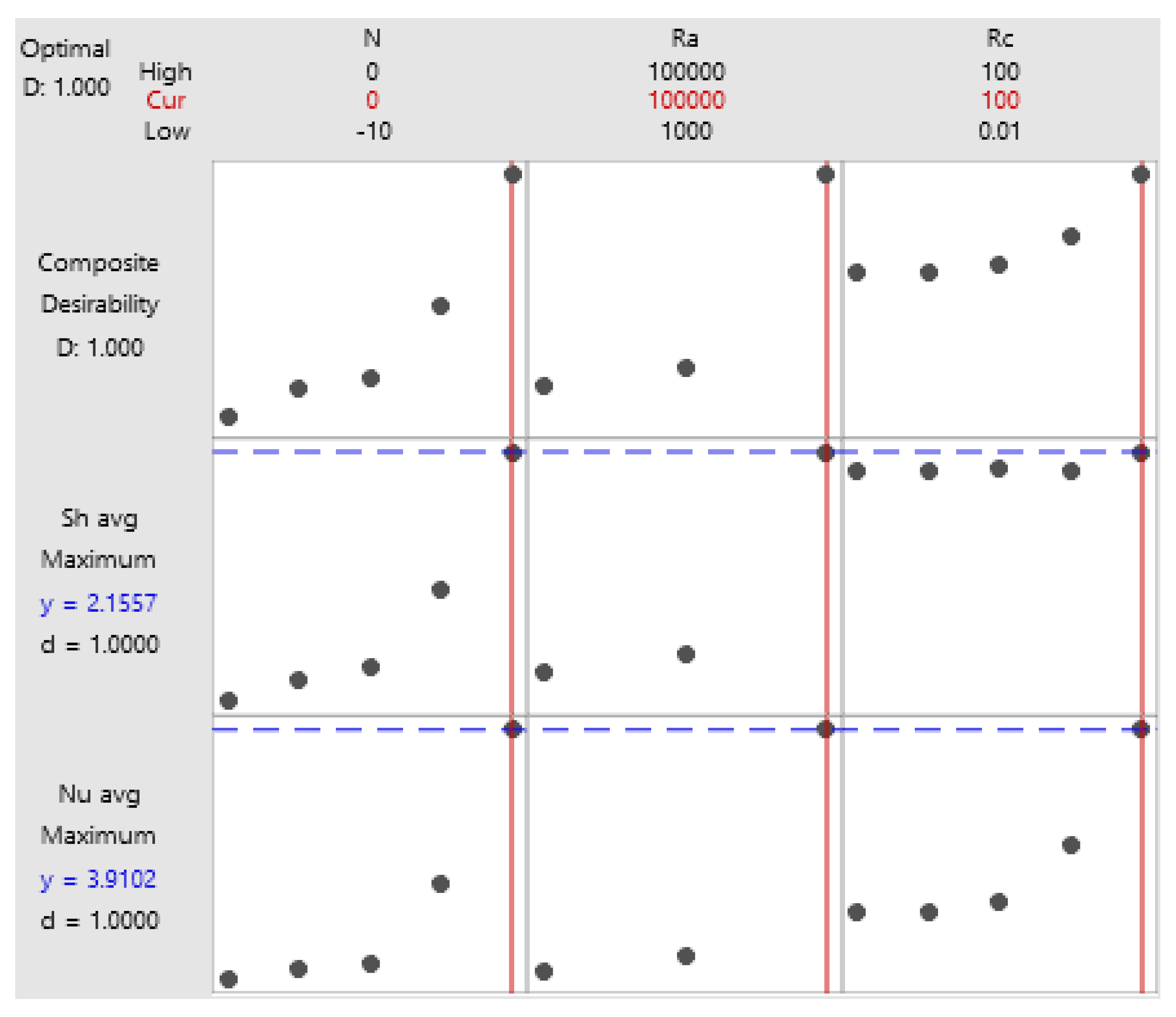
In order to determine the optimised solution for this current study, Figure 12 represents the response optimisation. The recommended solution is given in

Table 3. Multiple Response Prediction.

Variable	Setting
N	0
Ra	105
Rc	100
N	0

.

The recommended factor values to have the highest value of Nu_av are for N = 0, Ra = 10⁵ and Rc = 100. The same conditions were also deduced for Sh_av.

7. Conclusions

The 3D double diffusive convection in a finned solar still is studied numerically using the finite volume method and vector potential formalism. The main conclusions can be summarised as follows:

The flow structure is significatively influenced by varying the buoyancy ratio, conductivity ratio and Rayleigh number.

−

The intensity of the flow increases by increasing the conductivity of the fins.

−

The effect of fins conductivity on the temperature and concentration fields is negligible for high negative values of the buoyancy ratio.

−

The increase of Rc and Ra leads to the enhancement of the heat and mass transfers especially for low negative values of the buoyancy ratio.

−

The recommended factors value for Nu_av and Shav average are N = 0, Ra = 10⁵ and Rc = 100.

References

- Rahbar, N.; Esfahani, J.A.; Fotouhi-Bafghi, E. Estimation of convective heat transfer coefficient and water-productivity in a tubular solar still—CFD simulation and theoretical analysis. Sol. Energy 2015, 113, 313–323. [Google Scholar] [CrossRef]
- Mittal, G. An unsteady CFD modelling of a single slope solar still. Mater. Today Proc. 2021, 46, 10991–10995. [Google Scholar] [CrossRef]
- Esfe, M.H.; Toghraie, D. Numerical study on the effect of solar radiation intensity on the fresh water productivity of solar still equipped with Thermoelectric Cooling System (TEC) for hot and dry areas of Semnan. Case Stud. Therm. Eng. 2022, 32, 101848. [Google Scholar] [CrossRef]
- El-Sebaey, M.S.; Ellman, A.; Hegazy, A.; Ghonim, T. Experimental analysis and CFD modeling for conventional basin-type solar still. Energies 2020, 13, 5734. [Google Scholar] [CrossRef]
- Keshtkar, M.; Eslami, M.; Jafarpur, K. Effect of design parameters on performance of passive basin solar stills considering instantaneous ambient conditions: A transient CFD modeling. Sol. Energy 2020, 201, 884–907. [Google Scholar] [CrossRef]
- Setoodeh, N.; Rahimi, R.; Ameri, A. Modeling and determination of heat transfer coefficient in a basin solar still using CFD. Desalination 2011, 268, 103–110. [Google Scholar] [CrossRef]
- Khare, V.R.; Singh, A.P.; Kumar, H.; Khatri, R. Modelling and Performance Enhancement of Single Slope Solar Still Using CFD. Energy Procedia 2017, 109, 447–455. [Google Scholar] [CrossRef]
- Shoeibi, S.; Kargarsharifabad, H.; Rahbar, N.; Ahmadi, G.; Safaei, M.R. Performance evaluation of a solar still using hybrid nanofluid glass cooling-CFD simulation and environmental analysis. Sustain. Energy Technol. Assess. 2022, 49, 101728. [Google Scholar] [CrossRef]
- Keshtkar, M.; Eslami, M.; Jafarpur, K. A novel procedure for transient CFD modeling of basin solar stills: Coupling of species and energy equations. Desalination 2020, 481, 114350. [Google Scholar] [CrossRef]
- Gnanavel, C.; Saravanan, R.; Chandrasekaran, M. CFD analysis of solar still with PCM. Mater. Today Proc. 2020, 37, 694–700. [Google Scholar] [CrossRef]
- Yan, T.; Xie, G.; Liu, H.; Wu, Z.; Sun, L. CFD investigation of vapor transportation in a tubular solar still operating under vacuum. Int. J. Heat Mass Transf. 2020, 156, 119917. [Google Scholar] [CrossRef]
- Rahman, M.M.; Rahim, N.A.; Amin, N.; Saidur, R. A numerical model for the simulation of double-diffusive natural convection in a triangular solar collector. In Proceedings of the 2011 IEEE 1st Conference Clean Energy Technology CET, Kuala Lumpur, Malaysia, 27–29 June 2011; pp. 327–331. [Google Scholar] [CrossRef]
- Al-Rashed, A.A.; Oztop, H.F.; Kolsi, L.; Boudjemline, A.; Almeshaal, M.A.; Ali, M.E.; Chamkha, A. CFD study of heat and mass transfer and entropy generation in a 3D solar distiller heated by an internal column. Int. J. Mech. Sci. 2019, 152, 280–288. [Google Scholar] [CrossRef]
- Saleem, K.B.; Koufi, L.; Alshara, A.K.; Kolsi, L. Double-diffusive natural convection in a solar distiller with external fluid stream cooling. Int. J. Mech. Sci. 2020, 181, 105728. [Google Scholar] [CrossRef]
- Saleem, K.B.; Ghachem, K.; Koufi, L.; Kolsi, L. Analysis of Double-diffusive natural convection in a solar distiller embedded with PCM and cooled with external water stream. J. Taiwan Inst. Chem. Eng. 2021, 126, 67–79. [Google Scholar] [CrossRef]
- Alvarado-Juárez, R.; Álvarez, G.; Xamán, J.; Hernández-López, I. Numerical study of conjugate heat and mass transfer in a solar still device. Desalination 2013, 325, 84–94. [Google Scholar] [CrossRef]
- Alvarado-Juárez, R.; Xamán, J.; Álvarez, G.; Hernández-López, I. Numerical study of heat and mass transfer in a solar still device: Effect of the glass cover. Desalination 2015, 359, 200–211. [Google Scholar] [CrossRef]
- Rahman, M.M.; Saha, S.; Mojumder, S.; Rabbi, K.M.; Hasan, H.; Ibrahim, T.A. Unsteady double-diffusive buoyancy-induced flow in a triangular solar collector shape enclosure with corrugated bottom wall: Effects of buoyancy ratio. Int. J. Numer. Methods Heat Fluid Flow 2017, 27, 1282–1303. [Google Scholar] [CrossRef]
- Rahman, M.M.; Öztop, H.F.; Ahsan, A.; Kalam, M.A.; Varol, Y. Double-diffusive natural convection in a triangular solar collector. Int. Commun. Heat Mass Transf. 2012, 39, 264–269. [Google Scholar] [CrossRef]
- Ghachem, K.; Kolsi, L.; Mâatki, C.; Hussein, A.K.; Borjini, M.N. Numerical simulation of three-dimensional double diffusive free convection flow and irreversibility studies in a solar distiller. Int. Commun. Heat Mass Transf. 2012, 39, 869–876. [Google Scholar] [CrossRef]
- Ghachem, K.; Kolsi, L.; Larguech, S.; Alnemer, G. Heat and mass transfer enhancement in triangular pyramid solar still using CNT-water nanofluid. J. Cent. South Univ. 2021, 28, 3434–3448. [Google Scholar] [CrossRef]
- Purnachandrakumar, D.; Mittal, G.; Sharma, R.K.; Singh, D.B.; Tiwari, S.; Sinhmar, H. Review on Performance of Solar Stills Using Computational Fluid Dynamics (CFD); No. 0123456789; Springer: Berlin/Heidelberg, Germany, 2022. [Google Scholar]
- Mallinson, G.D.; Davis, G.D.V. Three-Dimensional Natural Convection in a Box: A Numerical Study. J. Fluid Mech. 1975, 83, 1–31. [Google Scholar] [CrossRef]
- Patankar, S.V. Numerical Heat Transfer and Fluid Flow, 1st ed.; Taylor & Francis: Philadelphia, PA, USA, 1980. [Google Scholar]
- Nishimura, T.; Wakamatsu, M.; Morega, A.M. Oscillatory double-diffusive convection in a rectangular enclosure with combined horizontal temperature and concentration gradients. Int. J. Heat Mass Transf. 1998, 41, 1601–1611. [Google Scholar] [CrossRef]