Development and Applications of Augmented Whale Optimization Algorithm

Abstract

Metaheuristics are proven solutions for complex optimization problems. Recently, bio-inspired metaheuristics have shown their capabilities for solving complex engineering problems. The Whale Optimization Algorithm is a popular metaheuristic, which is based on the hunting behavior of whale. For some problems, this algorithm suffers from local minima entrapment. To make WOA compatible with a number of challenging problems, two major modifications are proposed in this paper: the first one is opposition-based learning in the initialization phase, while the second is inculcation of Cauchy mutation operator in the position updating phase. The proposed variant is named the Augmented Whale Optimization Algorithm (AWOA) and tested over two benchmark suits, i.e., classical benchmark functions and the latest CEC-2017 benchmark functions for 10 dimension and 30 dimension problems. Various analyses, including convergence property analysis, boxplot analysis and Wilcoxon rank sum test analysis, show that the proposed variant possesses better exploration and exploitation capabilities. Along with this, the application of AWOA has been reported for three real-world problems of various disciplines. The results revealed that the proposed variant exhibits better optimization performance.

1. Introduction and Literature Review

Optimization is a process to fetch the best alternative solution from the given set of alternatives. Optimization processes are evident everywhere around of us. For example, to run a generating company, the operator has to take care of operating cost and to check and deal with various type of markets to execute financial transactions.The operator has to optimize the fuel purchase cost, sell the power at maximum rate and purchase the carbon credits at minimum cost to earn profit. Sometimes, optimization processes involve various stochastic variables to model the uncertainty in the process. Such processes are quite difficult to handle and often pose a severe challenge to the optimizer or solution provider algorithms. Evolution of modern optimizers is the outcome of these complex combinatorial multimodal nonlinear optimization problems. Unlike classical optimizers, where the search starts with the initial guess, these modern optimizers are based on the stochastic variables, and hence, they are less vulnerable towards local minima entrapment. These problems become the main source of emerging of metaheuristic algorithms, which are capable of finding a near-optimal solution in less computation time. The popularity of metaheuristic algorithms [1] has increased exponentially in the last two decades due to their simplicity, derivation-free mechanism, flexibility and better results providing capacity in comparison with conventional methods. The main inspiration of these algorithms is nature, and hence, aliased as nature-inspired algorithms [2].

Social mimicry of nature and living processes, behavior analysis of animals and cognitive viability are some of the attributes of nature-inspired algorithms. Darwin’s theory of evolution has inspired some nature-inspired algorithms, based on the property of “inheritance of good traits” and “competition, i.e., survival of the fittest”. These algorithms are Genetic Algorithm [3], Differential Evolution and Evolutionary Strategies [4].

The other popular philosophy is to mimic the behavior of animals which search for food. In these approaches, food or prey is used as a metaphor for global minima in mathematical terms. Exploration, exploitation and convergence towards the global minima is mapped with animal behavior. Most of the nature-inspired algorithms also known as population-based algorithms can further be classified as:

• Bio-inspired Swarm Intelligence (SI)-based algorithms: This category includes all algorithms inspired by any behavior of swarms or herds of animals or birds. Since most birds and animals live in a flock or group, there many algorithms that fall under this category, such as Ant Colony Optimization (ACO) [5], Artificial Bee Colony [6], Bat Algorithm [7], Cuckoo Search Algorithm [8], Krill herd Algorithm [9], Firefly Algorithm [10], Grey Wolf Optimizer [11], Bacterial Foraging Algorithm [12], Social Spider Algorithm [13], Cat Swarm Optimization [14], Moth Flame Optimization [15], Ant Lion Optimizer [16], Crow Search Algorithm [17] and Grasshopper Optimization Algorithm [18]. A social interaction-based algorithm named gaining and sharing knowledge was proposed in reference [19]. 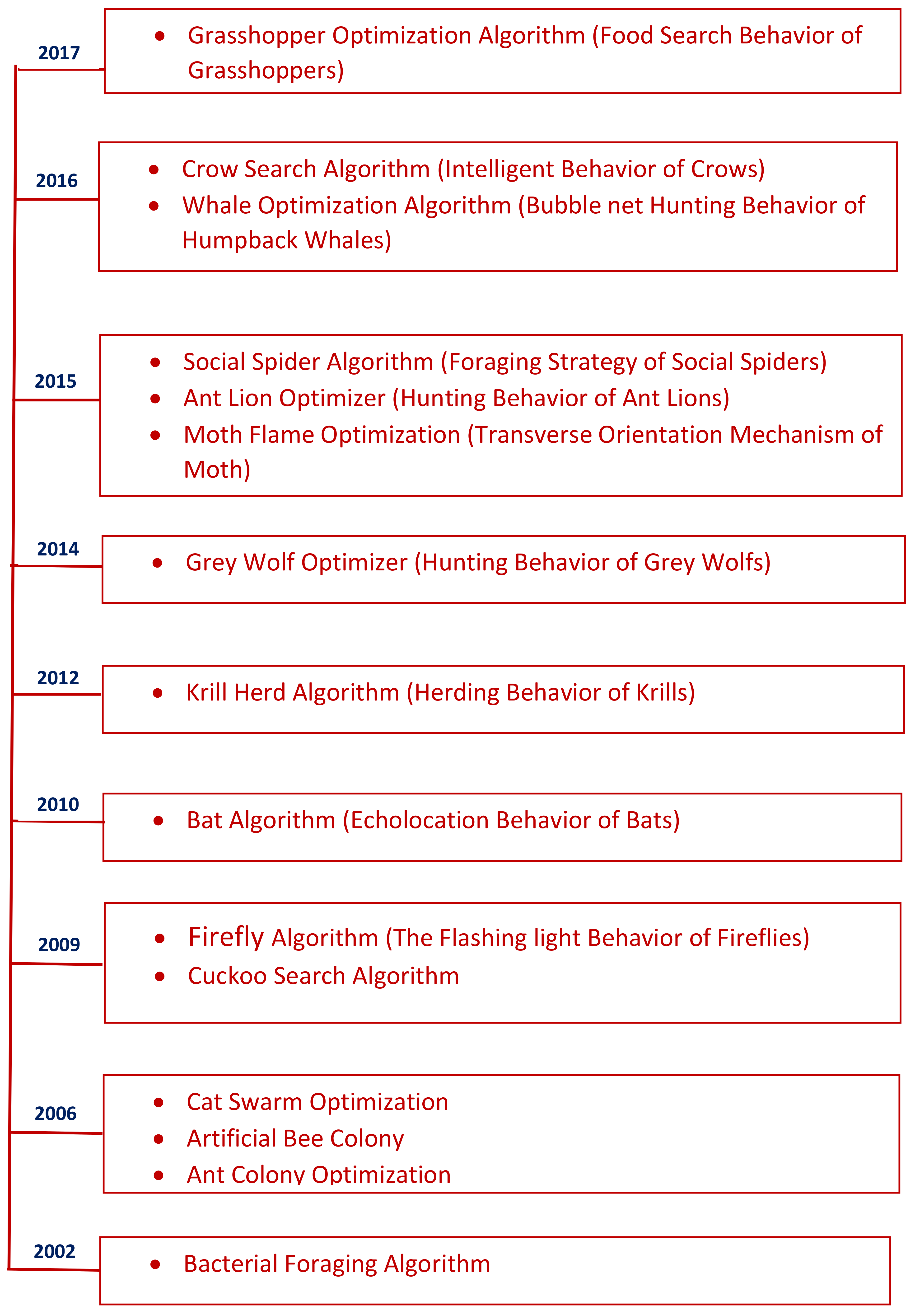References pertaining to the applications of bioinspired algorithms affirm the suitability of these algorithms on real-world problems [20,21,22,23]. A timeline of some famous bio-inspired algorithms is presented in Figure 1.
• Physics- or chemistry-based algorithms: Algorithms developed by mimicking any physical or chemical law fall under this category. Some of them are Big bang-big crunch Optimization [24], Black Hole [25], Gravitational search Algorithm [26], Central Force [27] and Charged system search [28].

Other than these population-based algorithms, a few different algorithms have also been proposed to solve specific mathematical problems. In [29,30], the authors proposed the concept of construction, solution and merging. Another Greedy randomised adaptive search-based algorithm using the improved version of integer linear programming was proposed in [31].

The No Free Lunch Theorem proposed by Wolpert et al. [32] states that there is no one metaheuristic algorithm which can solve all optimization problems. From this theorem, it can be concluded that there is no single metaheuristic that can provide the best solution for all problems. It is possible that one algorithm may be very effective for solving certain problems but ineffective in solving other problems. Due to the popularity of nature-inspired algorithms in providing reasonable solutions to complex real-life problems, many new nature-inspired optimization techniques are being proposed in the literature. It is interesting to note that all bio-inspired algorithms are subsets of nature-inspired algorithms. Among all of these algorithms, the popularity of bio-inspired algorithms has increased exponentially in recent years. Despite of this popularity, these algorithms have also been critically reviewed [33].

In 2016, Mirjalili et al. [34] proposed a new nature-inspired algorithm called the Whale optimization algorithm (WOA), inspired by the bubble-net hunting behavior of humpback whales. The humpback whale belongs to the rorqual family of whales, known for their huge size. An adult can be 12–16 m long and weigh 25–30 metric tons. They have a distinctive body shape and are known for their breaching behavior in water with astonishing gymnastic skills and for haunting songs sung by males during their migration period. Humpback whales eat small fish herds and krills. For hunting their prey, they follow a unique strategy of encircling the prey spirally, while gradually shrinking the size of the circles of this spiral. With incorporation of this theory, the performance of WOA is superior to many other nature-inspired algorithms. Recently, in [35], WOA was used to solve the optimization problem of the truss structure. WOA has also been used to solve the well-known economic dispatch problem in [36]. The problem of unit commitment from electric power generation was solved through WOA in [37]. In [38], the author applied WOA to the long-term optimal operation of a single reservoir and cascade reservoirs. The following are the main reasons to select WOA:

• There are few parameters to control, so it is easy to implement and very flexible.
• This algorithm has a specific characteristic to transit between exploration and exploitation phasesm as both of these include one parameter only.

Sometimes, it also suffers from a slow convergence speed and local minima entrapment due to the random size of the population. To overcome these shortcomings, in this paper, we propose two major modifications to the existing WOA:

• The first modification is the inculcation of the opposition-based learning (OBL) concept in the initialization phase of the search process, or in other words, the exploratory stage. The OBL is a proven tool for enhancing the exploration capabilities of metaheuristic algorithms.
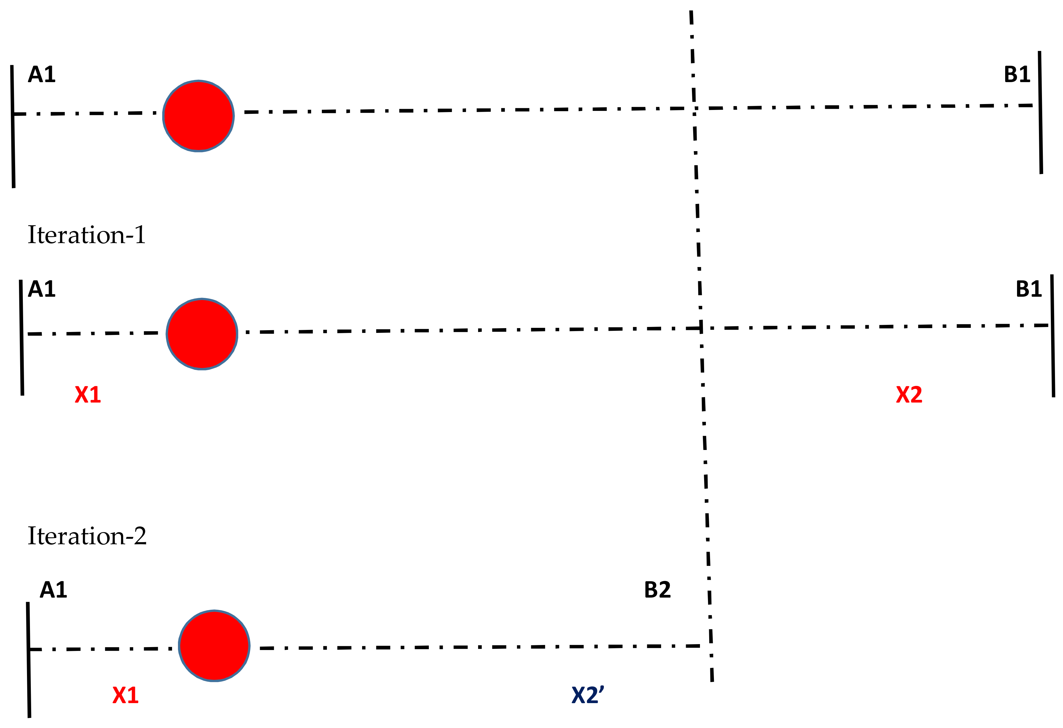
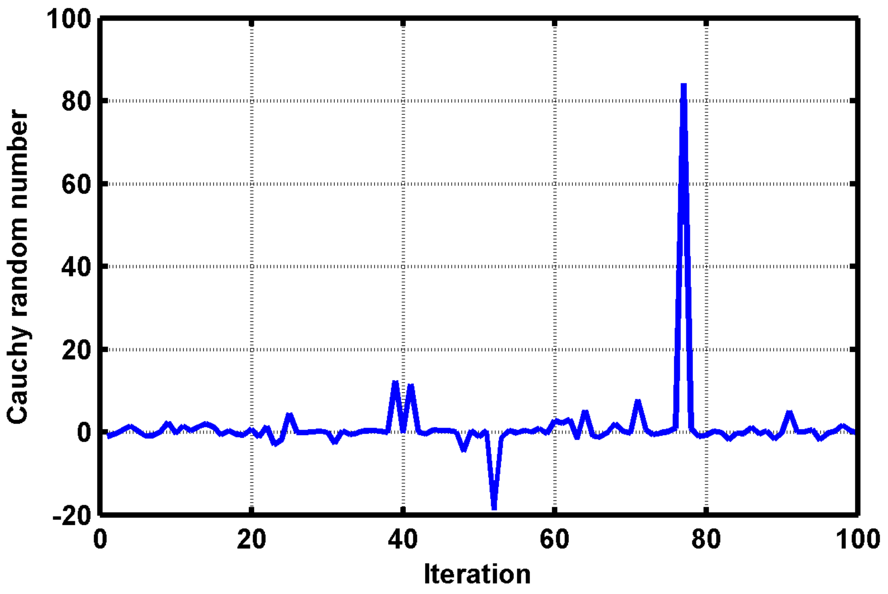
• The second modification is of the position updating phase, by updating the position vector with the help of Cauchy numbers.

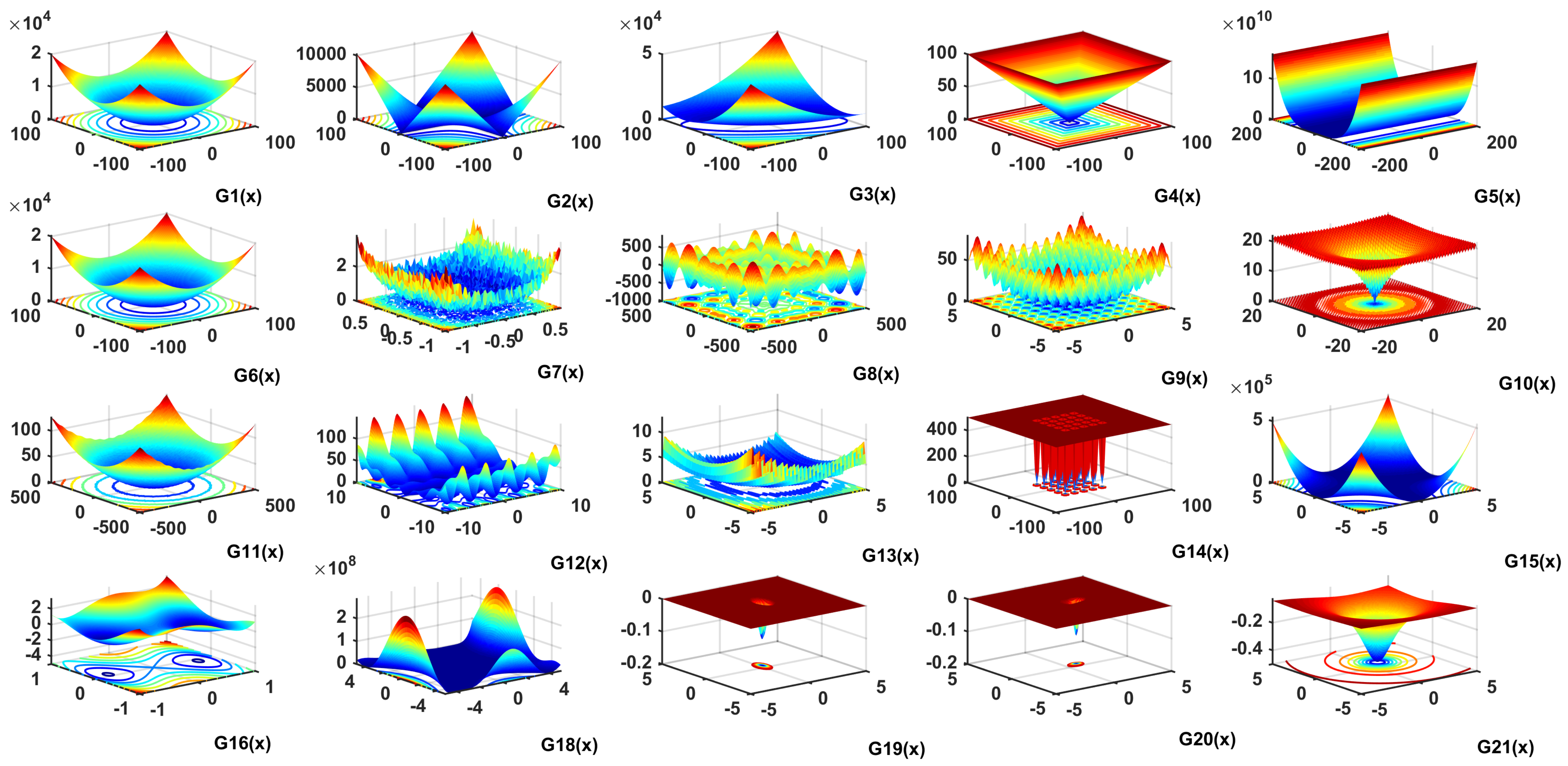
The remaining part of this paper is organized as follows: Section 2 describes the crisp mathematical details of WOA. Section 3 is a proposal of the proposed variant; an analogy based on modified position update is also established with the proposed mathematical framework. Section 4 includes the details of benchmark functions. In Section 5 and Section 6 show the results of the benchmark functions and some real-life problems that occur with different statistical analyses. Last but not the least, the paper concludes in Section 7 with a decisive evaluation of the results, and some future directions are indicated.

2. Mathematical Framework of WOA

The mathematical model of WOA can be presented in three steps: prey encircling, exploitation phase through bubble-net and exploration phase, i.e., prey search.

• Prey encircling: Humpback whales choose their target prey through the capacity to finding the location of prey. The best search agent is followed by other search agents to update their positions, which can be given mathematically as:

  $$\overrightarrow{P}=\left|\overrightarrow{Q}\overrightarrow{Y}*\left(s\right)-\overrightarrow{Y}\left(s\right)\right|$$

  (1)

  $$\overrightarrow{Y}\left(s+1\right)=\overrightarrow{Y}*\left(s\right)-\overrightarrow{R}·\overrightarrow{P}$$

  (2)

  where $Y^{\ast }$ denotes the position vector of the best obtained solution, $\overrightarrow{Y}$ is the position vector, s is the current iteration, $| |$ denotes the absolute value and · denotes the element to element multiplication.
  The coefficients $\overrightarrow{R}$ and $\overrightarrow{Q}$ can be calculated as follows:

  $$\overrightarrow{R}=2\overrightarrow{p}·\overrightarrow{r}-\overrightarrow{p}$$

  (3)

  $$\overrightarrow{Q}=2\overrightarrow{r}$$

  (4)

  where $\overrightarrow{p}$ linearly decreases with every iteration from 2 to 0 and $\overrightarrow{r}\in \left[0,1\right]$. By adjusting the values of vectors $\overrightarrow{P}$ and $\overrightarrow{R}$, the current position of search agents shifted towards the best position. This position updating process in the neighborhood direction also helps in encircling the prey n dimensionally.
• Exploitation phase through bubble-net: The value of $\overrightarrow{p}$ decreases in the interval $[-p,p]$. Due to changes in $\overrightarrow{p}$, $\overrightarrow{P}$ also fluctuates and represents the shrinking behavior of search agents. By choosing random values of $\overrightarrow{P}$ in the interval $[-1,1]$, the humpback whale updates its position. In this process, the whale swims towards the prey spirally and the circles of spirals slowly shrink in size. This shrinking of the spirals in a helix-shaped movement can be mathematically modeled as:

  $$\overrightarrow{Y}\left(s+1\right)={\overrightarrow{Q}}^{\prime }·e^{al}·cos\left(2\pi l\right)+\overrightarrow{Y}*\left(s\right)$$

  (5)

  $${\overrightarrow{Q}}^{\prime }=\left|\overrightarrow{Y}*(s)-\overrightarrow{Y}(s)\right|$$

  (6)

  where $\overrightarrow{a}$ is the constant factor responsible for the shape of spirals and l randomly belongs to interval $[-1,1]$.
  In the position updating phase, whales can choose any model, i.e., the shrinking mechanism or the spiral mechanism. The probability of this simultaneous behavior is assumed to be 50 during the optimization process. The combined equation of both of these behavior can be represented as:

  $$\overrightarrow{Y}\left(s+1\right)=\left\{\begin{array}{c}\overrightarrow{Y}*\left(s\right)-\overrightarrow{P}·\overrightarrow{Q}\hspace{1em}p<0.5\\ {\overrightarrow{Q}}^{\prime }{e}^{al}cos\left(2\pi l\right)+Y^s\hspace{1em}p>0.5\end{array}\right.$$

  (7)
• Exploration Phase
  In this phase, $\overrightarrow{P}$ is chosen opposite to the exploitation phase, i.e., the value of $\overrightarrow{P}$ must be >1 or <−1, so that the humpback whales can move away from each other, which increases the exploration rate. This phenomenon can be represented mathematically as:

  $$\overrightarrow{Q}=\left|\overrightarrow{R}·{\overrightarrow{Y}}_{rand}-\overrightarrow{Y}\right|$$

  (8)

  $$\overrightarrow{Y}\left(s+1\right)={\overrightarrow{Y}}_{rand}-\overrightarrow{P}·\overrightarrow{Q}$$

  (9)

  where ${\overrightarrow{Y}}_{rand}$ represents the position of a random whale.
  After achieving the termination criteria, the optimization process finishes. The main features of WOA are the presence of the dual theory of circular shrinking and spiral path, which increase the exploitation process of finding the best position around the prey. Afterwards, the exploration phase provides a larger area through the random selection of values of $\left|\overrightarrow{A}\right|$.

3. Motivation and Development of the Augmented Whale Optimization Algorithm

It is observed in the previous reported applications that inserting mutation in the population-based schemes can enhance the performance of the optimization. Some noteworthy applications are reported in [39].

3.1. Augmented Whale Optimization Algorithm (AWOA)

By taking the motivation of the modified position update, we present the development of AWOA and the mathematical steps we have incorporated. To simulate the behavior of whale through modified position update and their connection to the position update mechanism for mating, we require two mechanisms:

• The mechanism that puts the whales in diverse directions.
• The mechanism that updates the positions of the whales by using a mathematical signal.

3.1.1. The Opposition-Based Position Update Method

For simulating the first mechanism, we choose the opposition number generation theory that was proposed by H. R Tizoosh. Opposition-based learning is the concept that puts the search agents in diverse (rather opposite directions) so that the search for optima can also be initiated from opposite directions. This theory has been applied in many metaheuristic algorithms, and now, it is a proven fact that the search capabilities of the optimizer can substantially be enhanced by the application of this opposition number generation technique. Some recent papers have provided evidence of this [40,41]. With these approaches, an impact of opposition-based learning can be easily seen. Furthermore, a rich review on the techniques related to opposition, application area and performance-wise comparison can be read in [42,43].

The following points can be taken as some positive arguments in favor of the application of the oppositional number generation theory (ONGT) concept:

• While solving multimodal optimization problems, it is required that an optimizer should start a process from the point which is nearer to the global optima; in some cases, the loose position update mechanism becomes a potential cause for local minima entrapment. The ONGT becomes a helping hand in such situations, as it places search agents in diverse directions, and hence, the probability of local minima entrapment is substantially decreased.
• In real applications, where the shape and nature of objective functions are unknown, the ONGT can be a beneficial tool because if the function is unimodal in nature, as per the research, the exploration capabilities of any optimizers can be substantially enhanced by the application of ONGT. On the other hand, if the function is multimodal in nature, then ONGT will help search agents to acquire opposite positions and help the optimizer’s mechanism to converge to global optima.

For the reader’s benefit, we are incorporating some definitions of opposite points in search space for a 2D and multidimensional space.

Definition 1.

Let $x\in [a,b]$ be a real number, where the opposite number of x is defined by:

$$\stackrel{-}{x}=a+b-x$$

(10)

The same holds for Q dimensional space.

Definition 2.

Let $A=(x_1,x_2,\dots ,x_Q)$ be a point in Q dimensional space, where $x_1,x_2,\dots ,x_Q\in R$ and $x_i\in [a,b],i=1,2,\dots ,Q$; the opposite points matrix can be given by $\stackrel{-}{A} = [\stackrel{-}{x_1} ,\stackrel{-}{x_2} ,\stackrel{-}{x_3} \dots ,\stackrel{-}{x_Q}]$. Hence:

$$\stackrel{-}{x_i}=[a_i+b_i-x_i]$$

(11)

where $a_i$ and $b_i$ are the lower limit and upper limit, respectively. Furthermore, Figure 2 illustrates the search process of ONGT, where A1 and B1 are the search boundaries, and it shrinks as the iterative process progresses.

3.1.2. Position Updating Mechanism Based on the Cauchy Mutation Operator

For simulating the second mechanism, we require a signal that is a close replica of a whale song. In the literature, a significant amount of work has been done on the application of the Cauchy mutation operator due to the following reasons:

• Since the expectation of the Cauchy distribution is not defined, the variance of this distribution is infinite; due to this fact, the Cauchy operators sometimes generate a very long jump as compared to normally distributed random numbers [44,45]. This phenomenon can be observed in Figure 3.
• It is also shown in [44] that Cauchy distribution generates an offspring far from its parents; hence, the avoidance of local minima can be achieved.

In the proposed AWOA, the position update mechanism is derived from the Cauchy distribution operator. The Cauchy density function of the distribution is given by:

$$f_t\left(x\right)=\frac{1}{\pi } \frac{t}{t^2+x^2} -\infty < x < \infty$$

(12)

where t is the scaling parameter and the corresponding distribution function can be given as:

$$F_t\left(x\right)=\frac{1}{2}+\frac{1}{\pi }arctan\left(\frac{x}{t}\right)$$

(13)

First, a random number $y\in (0,1)$ is generated, after which a random number $\alpha$ is generated by using following equation:

$$\alpha =x_0+t tan\left(\pi (y-0.5)\right)$$

(14)

We assume that $\alpha$ is a whale position update generated by the search agents and on the basis of this signal, the position of the whale is updated. Furthermore, we define a position-based weight matrix of $jth$ position vector of $ith$ whale, which is given as:

$$W\left(j\right)=\frac{\left({\displaystyle \sum _{i=1}^{NP}}{x}_{i,j}\right)}{NP}$$

(15)

where $W\left(j\right)$ is a weight vector and NP is the population size of whale. Furthermore, the position update equation can be modified as:

$$x^{\prime }\left(j\right)=x\left(j\right)+W\left(j\right)\ast \alpha$$

(16)

Summarizing all the points discussed in this section, we propose two mechanisms for the improvement of the performance of WOA. The first one is the opposition-based learning concept that places whales in diverse directions to explore the search space effectively, and based on the whale behaviour(modified position update) is created by them, the position update mechanism is proposed. To simulate whale song, we employ Cauchy numbers. Hence, both of these mechanisms can be beneficial for enhancing the exploration and exploitation capabilities of WOA. In the next section, we will evaluate the performance of the proposed variant on some conventional and CEC-17 benchmark functions.

4. Benchmark Test Functions

Benchmark functions are a set of functions with different known characteristics (separability, modality and dimensionality) and often used to evaluate the performance of optimization algorithms. In the present paper, we measure the performance of our proposed variant AWOA through two benchmark suites.

• Benchmark Suite 1: In this suite, 23 conventional benchmark functions are considered, out of which 7 are unimodal and rest are multimodal and fixed dimension functions. The details of benchmark functions, such as mathematical definition, minima, dimensions and range are incorporated in

  Table 1. Details of Benchmark Functions Suite 1.

  Function	Dim	Range	Minima
  Unimodal Benchmark Function
  $G_1\left(x\right)={\displaystyle \sum _{i=1}^n}{x}_i^2$ (BF1)	30	[−100, 100]	0
  $G_2\left(x\right)={\displaystyle \sum _{i=1}^n}\left|x_i\right|+{\displaystyle \prod _{i=1}^n}\left|x_i\right|$ (BF2)	30	[−10, 10]	0
  $G_3\left(x\right)={\displaystyle \sum _{i=1}^n}{\left({\displaystyle \sum _{j-1}^i}{x}_j\right)}^2$ (BF3)	30	[−100, 100]	0
  $G_4\left(x\right)={max}_i\left\{\left|x_i\right|\hspace{1em}1\le i\le n\right.$ (BF4)	30	[−100, 100]	0
  $G_5\left(x\right)={\displaystyle \sum _{i=1}^{n-1}}[100{(x_{i+1}-x_i^2)}^2+{(x_i-1)}^2]$ (BF5)	30	[−30, 30]	0
  $G_6\left(x\right)={\displaystyle \sum _{i=1}^{n-1}}{\left([x_i+0.5]\right)}^2$ (BF6)	30	[−100, 100]	0
  $G_7\left(x\right)={\displaystyle \sum _{i=1}^{n-1}}i{x}_i^4+random[0,1]$ (BF7)	30	[−1.28, 1.28]	0
  Multimodal Benchmark Function
  $G_8\left(x\right)={\displaystyle \sum _{i=1}^n}-x_{i}sin\left(\sqrt{\left|z_i\right|}\right)$ (BF8)	30	[−500, 500]	−418.9829 × 5
  $G_9\left(x\right)={\displaystyle \sum _{i=1}^n}\left[{x_i}^2-10 cos\left(2\pi x_i\right)+10\right]$ (BF9)	30	[−5.12, 5.12]	0
  $G_{10}\left(x\right)=-20exp\left(-0.2\sqrt{\frac{1}{n}{\displaystyle \sum _{i=1}^n}{x_i}^2}\right)-exp\left(\frac{1}{n}{\displaystyle \sum _{i=1}^n}cos\left(2\pi x_i\right)\right)+20+e$ (BF10)	30	[−32, 32]	0
  $G_{11}\left(x\right)=\frac{1}{4000}{\displaystyle \sum _{i=1}^n}{x_i}^2-{\displaystyle \prod _{i=1}^n}cos\left(\frac{x_i}{\sqrt{i}}\right)+1$ (BF11)	30	[−600, 600]	0
  $G_{12}\left(x\right)=\frac{\pi }{n}\left\{10sin\left(\pi y_1\right)+{\displaystyle \sum _{i=1}^{n-1}}{(y_i-1)}^2[1+10{sin}^2\left(\pi y_{i+1}\right)]+{(y_n-1)}^2\right\}+{\displaystyle \sum _{i=1}^n}u(x_i,10,100,4)$ (BF12)	30	[−50, 50]	0
  $y_i=1+\frac{x_{i+1}}{4}$
  $u(x_i,a,k,m)=\left\{\begin{array}{cc}k{(x_i-a)}^m& x_i>a\\ 0& -a<x_i<a\\ k{(-x_i-a)}^m& x_i<-a\end{array}\right.$
  $G_{13}\left(x\right)=0.1\{si{n}^2\left(3\pi x_1\right)+{\displaystyle \sum _{i=1}^n}{(x_i-1)}^2[1+{sin}^2(3\pi x_i+1)]+{(x_n-1)}^2[1+{sin}^2\left(2\pi x_n\right)]\}+{\displaystyle \sum _{i=1}^n}u(x_i,5,100,4)$ (BF13)	30	[−50, 50]	0
  Fixed-Dimension Multimodal Benchmark Function
  $G_{14}\left(x\right)={\left(\frac{1}{500}+{\displaystyle \sum _{j=1}^{25}}\frac{1}{j+{\displaystyle \sum _{i=1}^2}{(x_i-a_{ij})}^6}\right)}^{-1}$ (BF14)	2	[−65, 65]	1
  $G_{15}\left(x\right)={{\displaystyle \sum _{j=1}^{11}}\left[a_i-\frac{x_1\left(b_i^2+b_i{x}_2\right)}{b_i^2+b_i{x}_3+x_4}\right]}^2$ (BF15)	4	[−5, 5]	0.00030
  $G_{16}\left(x\right)=4x_1^2-2.1x_1^4+\frac{1}{3}{x}_1^6+x_1{x}_2-4x_2^2+4x_2^4$ (BF16)	2	[−5, 5]	−1.0316
  $G_{17}\left(x\right)={\left(x_2-\frac{5.1}{4{\pi }^2}{x}_1^2+\frac{5}{\pi }{x}_1-6\right)}^2+10\left(1-\frac{1}{8\pi }\right)cos{x}_1+10$ (BF17)	2	[−5, 5]	0.398
  $G_{18}\left(x\right)=A\left(z\right)\times B\left(x\right)$
  $A\left(x\right)=1+{(x_1+x_2+1)}^2(19-14x_1+3x_1^2-14x_2+6x_1{x}_2+3x_2^2)$
  $B\left(x\right)=30+{(2x_1-3x_2)}^2\times (18-32x_1+12x_1^2+48x_2-36x_1{x}_2+27x_2^2)$ (BF18)	2	[−2, 2]	3
  $G_{19}\left(x\right)=-{\displaystyle \sum _{i=1}^4}{c}_{i}exp\left(-{\displaystyle \sum _{j=1}^3}{a}_{ij}{(x_j-p_{ij})}^2\right)$ (BF19)	3	[1, 3]	−3.86
  $G_{20}\left(x\right)=-{\displaystyle \sum _{i=1}^4}{c}_{i}exp\left(-{\displaystyle \sum _{j=1}^6}{a}_{ij}{(x_j-p_{ij})}^2\right)$ (BF20)	6	[0, 1]	−3.32
  $G_{21}\left(x\right)=-{\displaystyle \sum _{i=1}^5}{\left[(X-a_i){(X-a_i)}^T+c_i\right]}^{-1}$ (BF21)	4	[0, 10]	−10.1532
  $G_{22}\left(x\right)=-{{\displaystyle \sum _{i=1}^7}\left[(X-a_i){(X-a_i)}^T+c_i\right]}^{-1}$ (BF22)	4	[0, 10]	−10.4028
  $G_{23}\left(x\right)=-{{\displaystyle \sum _{i=1}^{10}}\left[(X-a_i){(X-a_i)}^T+c_i\right]}^{-1}$ (BF23)	4	[0, 10]	−10.5363

  . For further details, one can refer to [46,47,48]. The shapes of the used benchmark functions are given in Figure 4.
• Benchmark Suite 2: For further benchmarking our proposed variant, we also choose a set of 29 functions of diverse nature from CEC 2017.

  Table 2. Details of CEC-2017 (Benchmark Suite 2).

  Function Name	Optima
  Unimodal Functions
  Shifted and Rotated Bent Cigar Function (CEC-G1) (F1)	100
  Shifted and Rotated Zakharov Function (CEC-G3) (F3)	300
  Simple Multimodal Functions
  Shifted and Rotated Rosenbrock’s Function (CEC-G4) (F4)	400
  Shifted and Rotated Rastrigin’s Function (CEC-G5) (F5)	500
  Shifted and Rotated Expanded Scaffer’s Function (CEC-G6) (F6)	600
  Shifted and Rotated Lunacek Bi Rastrigin Function (CEC-G7) (F7)	700
  Shifted and Rotated Non-continuous Rastrigin Function (CEC-G8) (F8)	800
  Shifted and Rotated Levy Function (CEC-G9) (F9)	900
  Shifted and Rotated Schwefel’s Function (CEC-G10) (F10)	1000
  Hybrid Functions
  Hybrid Function 1 (N = 3) (CEC-G11) (F11)	1100
  Hybrid Function 2 (N = 3) (CEC-G12) (F12)	1200
  Hybrid Function 3 (N = 3) (CEC-G13) (F13)	1300
  Hybrid Function 4 (N = 4) (CEC-G14) (F14)	1400
  Hybrid Function 5 (N = 4) (CEC-G15) (F15)	1500
  Hybrid Function 6 (N = 4) (CEC-G16) (F16)	1600
  Hybrid Function 7 (N = 5) (CEC-G17) (F17)	1700
  Hybrid Function 8 (N = 5) (CEC-G18) (F18)	1800
  Hybrid Function 9 (N = 5) (CEC-G19) (F19)	1900
  Hybrid Function 10 (N = 6) (CEC-G20) (F20)	2000
  Composite Functions
  Composition Function 1 (N = 3) (CEC-G21) (F21)	2100
  Composition Function 2 (N = 3) (CEC-G22) (F22)	2200
  Composition Function 3 (N = 4) (CEC-G23) (F23)	2300
  Composition Function 4 (N = 4) (CEC-G24) (F24)	2400
  Composition Function 5 (N = 5) (CEC-G25) (F25)	2500
  Composition Function 6 (N = 5) (CEC-G26) (F26)	2600
  Composition Function 7 (N = 6) (CEC-G27) (F27)	2700
  Composition Function 8 (N = 6) (CEC-G28) (F28)	2800
  Composition Function 9 (N = 3) (CEC-G29) (F29)	2900
  Composition Function 10 (N = 3) (CEC-G30) (F30)	3000

  showcases the minor details of these functions. For other details, such as optima and mathematical definitions, we can follow [49].

5. Result Analysis

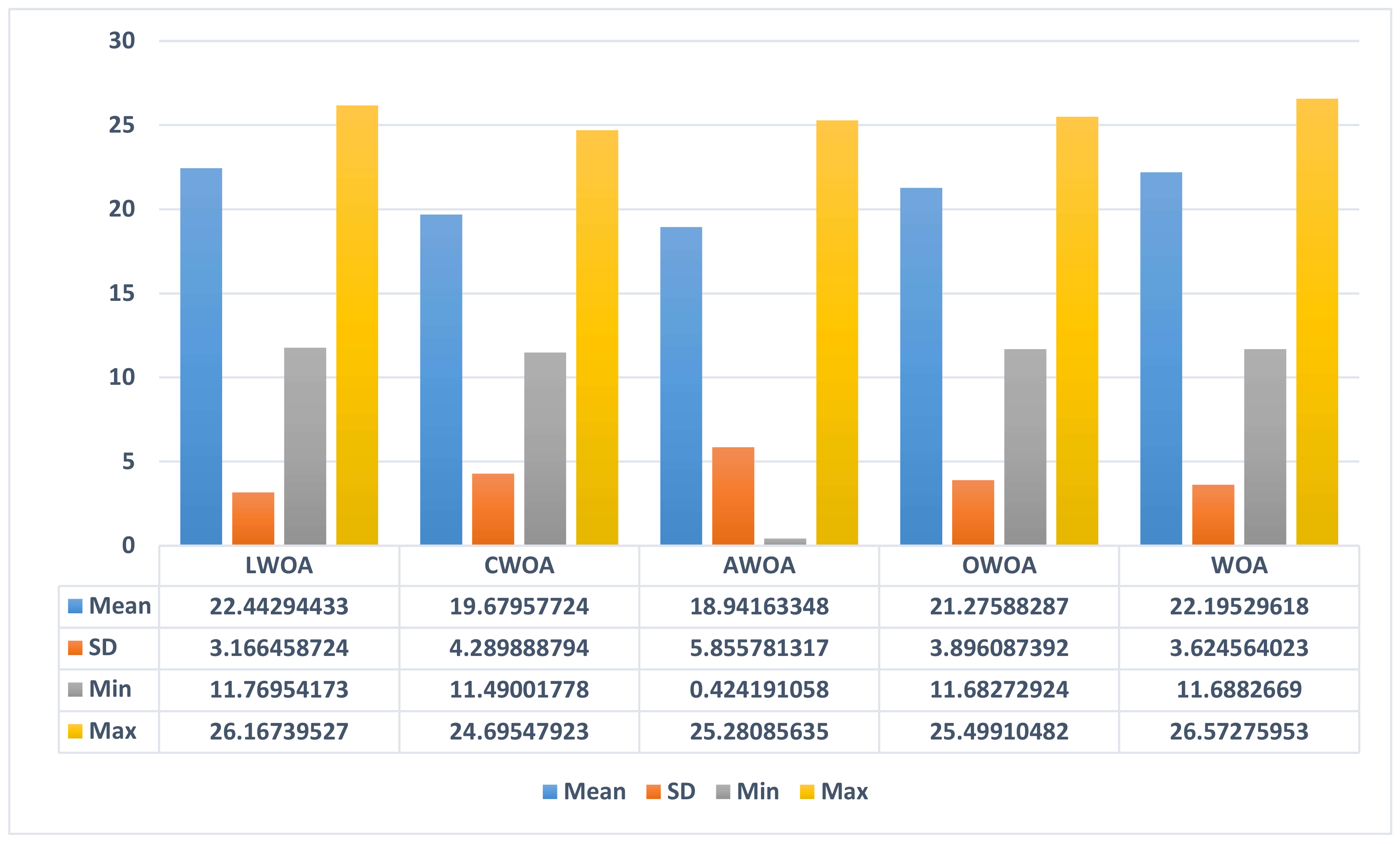
In this section, various analyses that can check the efficacy of the proposed modifications are exhibited. For judging the optimization performance of the proposed AWOA, we have chosen some recently developed variants of WOA for comparison purpose. These variants are:

• Lévy flight trajectory-based whale optimization algorithm (LWOA) [50].
• Improved version of the whale optimization algorithm that uses the opposition-based learning, termed OWOA [41].
• Chaotic Whale Optimization Algorithm (CWOA) [51].

5.1. Benchmark Suite 1

Table 3. Results of Benchmark Suite-1.

Function	Parameter	AWOA	CWOA	LWOA	OWOA	WOA
BF1	Mean	0.00	1.33 × ${10}^{-97}$	2.04 × ${10}^{-8}$	2.37 × ${10}^{-172}$	1.24 × ${10}^{-172}$
	SD	0.00	4.06 × ${10}^{-97}$	2.30 × ${10}^{-8}$	0.00	0.00
BF2	Mean	2.71 × ${\mathbf{10}}^{-\mathbf{297}}$	1.96 × ${10}^{-59}$	2.77 × ${10}^{-4}$	4.15 × ${10}^{-117}$	3.96 × ${10}^{-120}$
	SD	0.00	4.93 × ${10}^{-59}$	1.35 × ${10}^{-4}$	1.01 × ${10}^{-116}$	1.51 × ${10}^{-119}$
BF3	Mean	0.00	9.27 × ${10}^3$	8.11 × ${10}^2$	6.04 × ${10}^3$	7.02 × ${10}^3$
	SD	0.00	9.34 × ${10}^3$	5.41 × ${10}^2$	4.82 × ${10}^3$	6.55 × ${10}^3$
BF4	Mean	3.6 × ${\mathbf{10}}^{-\mathbf{313}}$	1.39 × ${10}^{-2}$	5.88 × ${10}^{-1}$	8.02 × 10	4.74
	SD	0.00	5.71 × ${10}^{-2}$	3.38 × ${10}^{-1}$	1.98 × 10	1.33 × 10
BF5	Mean	2.84 × 10	2.78 × 10	2.77 × 10	2.71 × $\mathbf{10}$	2.74 × 10
	SD	6.08 × ${10}^{-1}$	6.12 × ${10}^{-1}$	2.32 × ${\mathbf{10}}^{-\mathbf{1}}$	8.95 × ${10}^{-1}$	9.66 × ${10}^{-1}$
BF6	Mean	4.49 × ${10}^{-1}$	1.36 × ${10}^{-97}$	2.73 × ${\mathbf{10}}^{-\mathbf{3}}$	5.46 × ${10}^{-1}$	5.02 × ${10}^{-1}$
	SD	2.01 × ${10}^{-1}$	4.81 × ${10}^{-1}$	1.09 × ${\mathbf{10}}^{-\mathbf{3}}$	2.46 × ${10}^{-1}$	3.71 × ${10}^{-1}$
BF7	Mean	1.55 × ${\mathbf{10}}^{-\mathbf{4}}$	4.94 × ${10}^{-4}$	7.58 × ${10}^{-3}$	1.53 × ${10}^{-3}$	1.75 × ${10}^{-3}$
	SD	1.87 × ${\mathbf{10}}^{-\mathbf{4}}$	4.88 × ${10}^{-4}$	6.70 × ${10}^{-3}$	1.96 × ${10}^{-3}$	1.93 × ${10}^3$
BF8	Mean	−7.80 × ${10}^3$	−6.93 × ${10}^3$	−9.50 × ${10}^3$	−1.03 × ${10}^4$	−9.02 × ${\mathbf{10}}^{\mathbf{3}}$
	SD	1.70 × ${10}^3$	1.51 × ${\mathbf{10}}^{\mathbf{3}}$	1.59 × ${10}^3$	2.13 × ${10}^3$	2.02 × ${10}^3$
BF9	Mean	0.00	0.00	1.88	0.00	2.84 × ${10}^{-15}$
	SD	0.00	0.00	4.94	0.00	1.27 × ${10}^{-14}$
BF10	Mean	8.88 × ${\mathbf{10}}^{-\mathbf{16}}$	4.80 × ${10}^{-15}$	8.75 × ${10}^{-5}$	4.09 × ${10}^{-15}$	4.09 × ${10}^{-15}$
	SD	0.00	2.28 × ${10}^{-15}$	3.34 × ${10}^{-5}$	1.59 × ${10}^{-15}$	2.55 × ${10}^{-15}$
BF11	Mean	0.00	5.58 × ${10}^{-3}$	2.09 × ${10}^{-3}$	0.00	0.00
	SD	0.00	2.50 × ${10}^{-2}$	6.61 × ${10}^{-3}$	0.00	0.00
BF12	Mean	2.03 × ${10}^{-2}$	7.91 × ${10}^{-2}$	2.28 × ${\mathbf{10}}^{-\mathbf{4}}$	3.44 × ${10}^{-2}$	3.64 × ${10}^{-2}$
	SD	9.28 × ${10}^{-3}$	3.22 × ${10}^{-2}$	7.37 × ${\mathbf{10}}^{-\mathbf{5}}$	2.11 × ${10}^{-2}$	2.35 × ${10}^{-2}$
BF13	Mean	5.69 × ${10}^{-1}$	1.23	8.76 × ${\mathbf{10}}^{-\mathbf{3}}$	9.87 × ${10}^{-1}$	1.01
	SD	1.97 × ${10}^{-1}$	3.56 × ${10}^{-1}$	6.05 × ${\mathbf{10}}^{-\mathbf{3}}$	2.51 × ${10}^{-1}$	3.37 × ${10}^{-1}$
BF14	Mean	2.14	1.89	1.05	3.16	2.77
	SD	9.80 × ${10}^{-1}$	1.01	2.22 × ${\mathbf{10}}^{\mathbf{3}}$	3.41	2.88
BF15	Mean	4.00 × ${\mathbf{10}}^{-\mathbf{4}}$	4.00 × ${10}^{-4}$	5.30 × ${10}^{-4}$	5.21 × ${10}^{-4}$	1.51 × ${10}^{-3}$
	SD	3.77 × ${10}^{-4}$	2.82 × ${10}^{-4}$	2.70 × ${10}^{-4}$	2.39 × ${\mathbf{10}}^{-\mathbf{4}}$	4.05 × ${10}^{-3}$
BF16	Mean	−1.03	−1.03	−1.03	−1.03	−1.03
	SD	1.57 × ${10}^{-8}$	1.12 × ${10}^{-8}$	2.32 × ${10}^{-8}$	6.20 × ${\mathbf{10}}^{-\mathbf{11}}$	7.34 × ${10}^{-11}$
BF17	Mean	3.98 × ${\mathbf{10}}^{-\mathbf{1}}$	3.98 × ${10}^{-1}$	3.98 × ${10}^{-1}$	3.98 × ${10}^{-1}$	3.98 × ${10}^{-1}$
	SD	1.73 × ${10}^{-8}$	8.73 × ${\mathbf{10}}^{-\mathbf{9}}$	4.40 × ${10}^{-6}$	1.39 × ${10}^{-7}$	1.23 × ${10}^{-6}$
BF18	Mean	3.00	3.00	3.00	3.00	3.00
	SD	1.12 × ${10}^{-4}$	1.30 × ${10}^{-4}$	9.86 × ${\mathbf{10}}^{-\mathbf{7}}$	3.88 × ${10}^{-5}$	4.88 × ${10}^{-5}$
BF19	Mean	−3.86	−3.86	−3.86	−3.86	−3.86
	SD	3.81 × ${10}^{-3}$	3.61 × ${10}^{-3}$	4.01 × ${\mathbf{10}}^{-\mathbf{5}}$	3.09 × ${10}^{-3}$	1.75 × ${10}^{-3}$
BF20	Mean	−3.22	−3.24	−3.27	−3.27	−3.23
	SD	1.30 × ${10}^{-1}$	8.36 × ${10}^{-1}$	6.38 × ${\mathbf{10}}^{-\mathbf{2}}$	7.17 × ${10}^{-2}$	1.23 × ${10}^{-1}$
BF21	Mean	−6.56	−7.74	−7.51	−8.27	−8.50
	SD	2.35	2.70	3.41	3.34	2.64
BF22	Mean	−8.71	−6.58	−8.62	−6.38	−8.03
	SD	3.04	2.97	2.83	3.48	3.42
BF23	Mean	−5.85	−7.20	−7.83	−7.79	−7.47
	SD	2.87	3.15	2.77	3.20	3.22

shows the optimization results of AWOA on Benchmark Suite 1 along with the leading. The table shows entries of mean and standard deviation (SD) of function values of 30 independent runs. Maximum function evaluations are set to 15,000. The first four functions in the table are unimodal functions. Benchmarking of any algorithm on unimodal functions gives us the information of the exploration capabilities of the algorithm. Inspecting the results of proposed AWOA on unimodal functions, it can be easily observed that the mean values are very competitive for the proposed AWOA as compared with other variants of WOA.

For rest of the functions, indicated mean values are competitive and the best results are indicated in bold face. From this statistical analysis, we can easily derive a conclusion that proposed modifications in AWOA are meaningful and yield positive implications on optimization performance of the AWOA specially on unimodal functions. Similarly, for multimodal functions BF-7 and BF-9 to 11, BF-15 to 19 and BF-22 have optimal values of mean parameter. We observed that the values of mean are competitive for rest of the functions and performance of proposed AWOA has not deteriorated.

5.1.1. Convergence Property Analysis

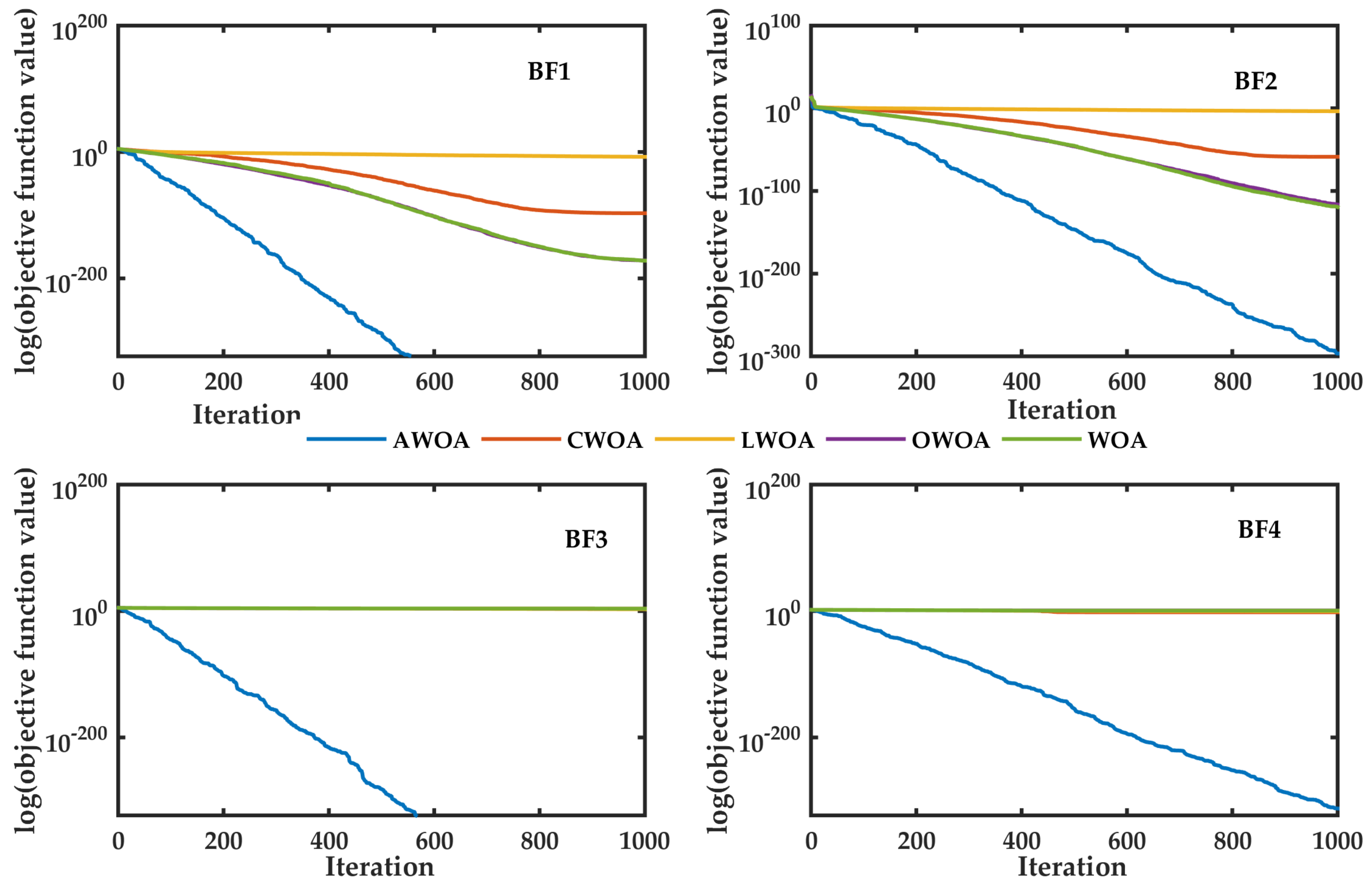
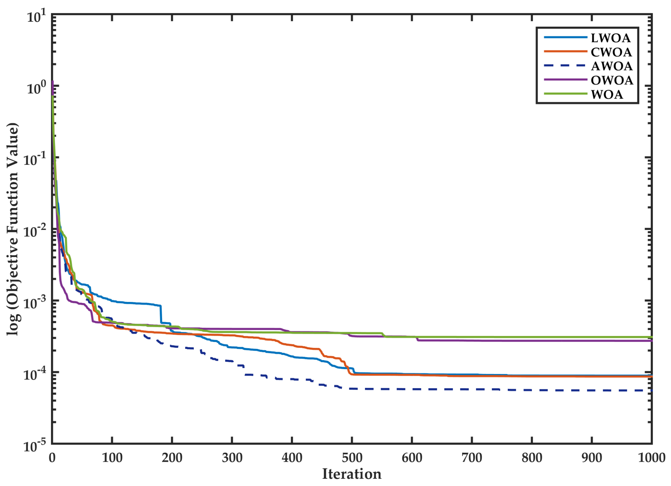
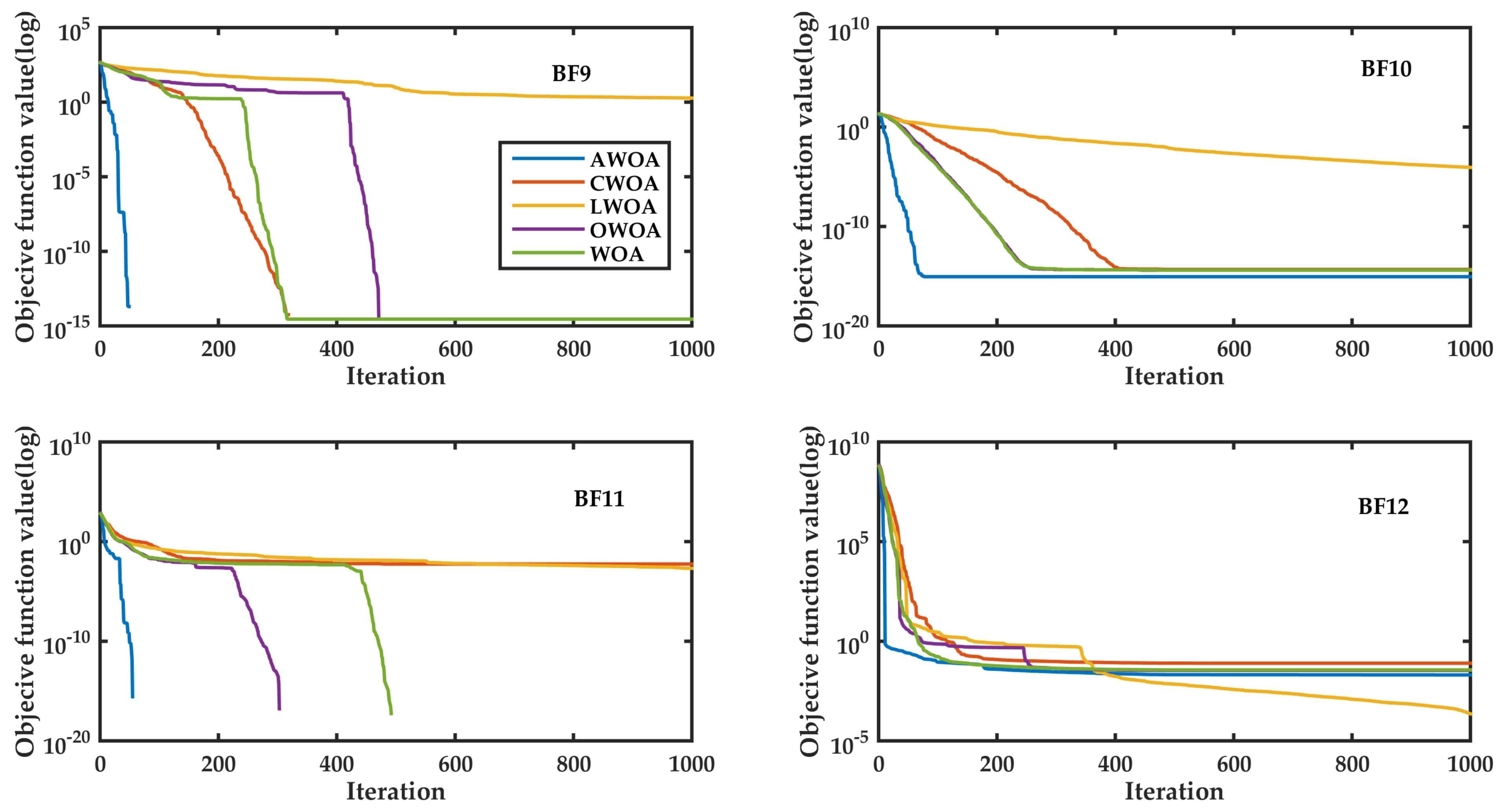
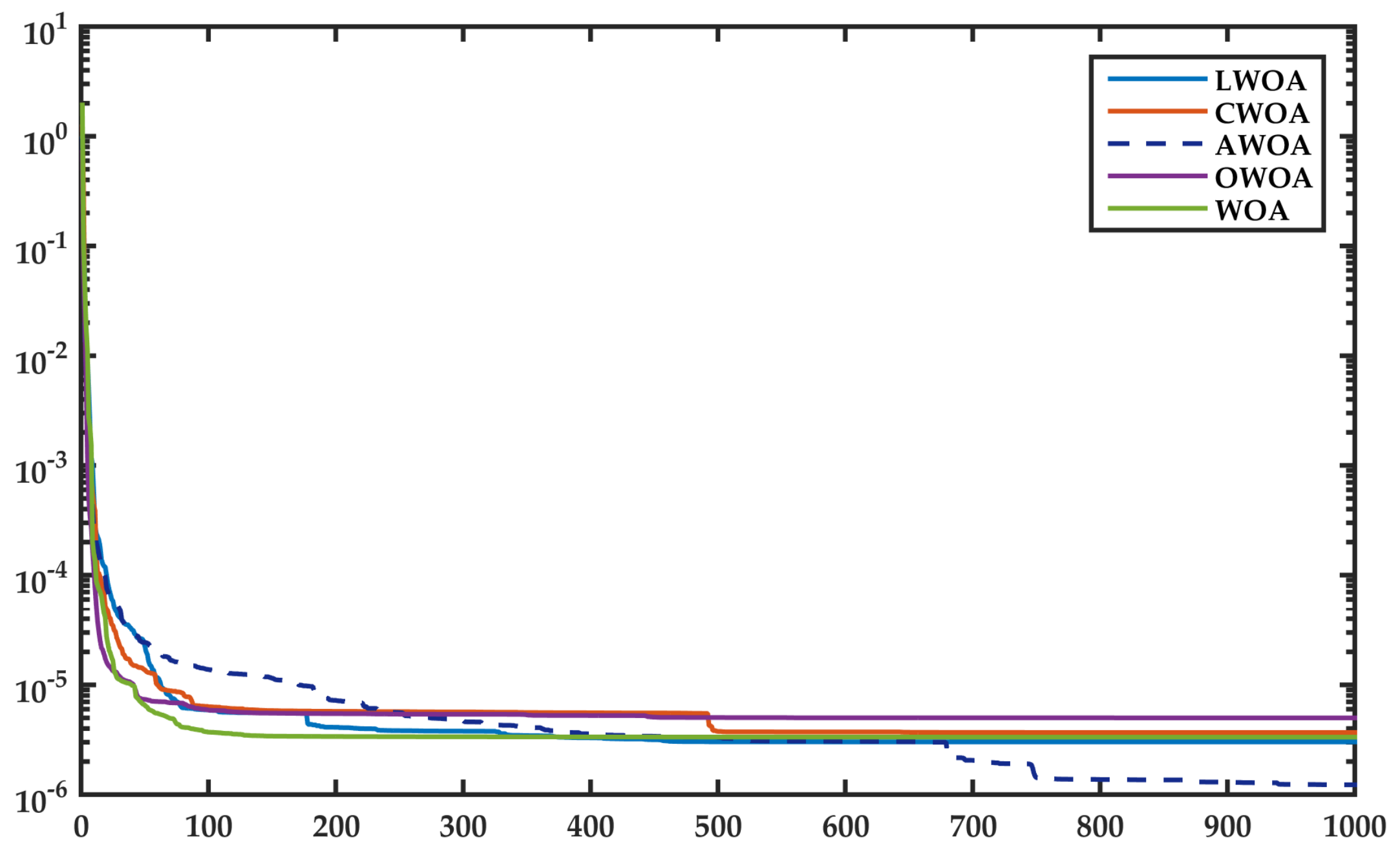
Similarly, the convergence plots for functions BF1 to BF4 have also been plotted in Figure 5 for the sake of clarity. From these convergence curves, it is observed that the proposed variant shows better convergence characteristics and the proposed modifications are fruitful to enhance the convergence and exploration properties of WOA. As it can be seen that convergence properties of AWOA is very swift as compared to other competitors. It is to be noted here that BF1–BF4 are unimodal functions and performance of AWOA on unimodal functions indicates enhanced exploitation properties. Furthermore, for showcasing the optimization capabilities of AWOA on multimodal functions the plots of convergence are exhibited in Figure 6. These are plotted for BF9 to BF12. From these results of proposed AWOA, it can easily be concluded that the results are also competitive.

5.1.2. Wilcoxon Rank Sum Test

A rank sum test analysis has been conducted and the p-values of the test are indicated in

Table 4. Results of Wilcoxon rank sum test of AWOA.

Function	CWOA	LWOA	OWOA	WOA
BF1	8.01 × ${\mathbf{10}}^{-\mathbf{9}}$	8.01 × ${10}^{-9}$	8.01 × ${10}^{-9}$	8.01 × ${10}^{-9}$
BF2	5.73 × ${\mathbf{10}}^{-\mathbf{8}}$	5.73 × ${\mathbf{10}}^{-\mathbf{8}}$	5.73 × ${\mathbf{10}}^{-\mathbf{8}}$	5.73 × ${\mathbf{10}}^{-\mathbf{8}}$
BF3	8.01 × ${\mathbf{10}}^{-\mathbf{9}}$	8.01 × ${\mathbf{10}}^{-\mathbf{9}}$	8.01 × ${\mathbf{10}}^{-\mathbf{9}}$	8.01 × ${\mathbf{10}}^{-\mathbf{9}}$
BF4	1.96 × ${\mathbf{10}}^{-\mathbf{8}}$	1.96 × ${\mathbf{10}}^{-\mathbf{8}}$	1.96 × ${\mathbf{10}}^{-\mathbf{8}}$	1.96 × ${\mathbf{10}}^{-\mathbf{8}}$
BF5	2.14 × ${10}^{-3}$	2.22 × ${10}^{-4}$	4.68 × ${\mathbf{10}}^{-\mathbf{5}}$	3.38 × ${10}^{-4}$
BF6	2.22 × ${10}^{-7}$	6.80 × ${\mathbf{10}}^{-\mathbf{8}}$	1.99 × $10$	9.46 × ${10}^{-1}$
BF7	8.36 × ${\mathbf{10}}^{-\mathbf{4}}$	7.90 × ${\mathbf{10}}^{-\mathbf{8}}$	2.92 × ${\mathbf{10}}^{-\mathbf{5}}$	6.01 × ${\mathbf{10}}^{-\mathbf{7}}$
BF8	1.20 × ${10}^{-1}$	6.04 × ${\mathbf{10}}^{-\mathbf{3}}$	7.58 × ${\mathbf{10}}^{-\mathbf{4}}$	1.02 × ${10}^{-1}$
BF9		8.01 × ${\mathbf{10}}^{-\mathbf{9}}$		3.42 × ${10}^{-1}$
BF10	2.14 × ${\mathbf{10}}^{-\mathbf{7}}$	8.01 × ${\mathbf{10}}^{-\mathbf{9}}$	1.11 × ${\mathbf{10}}^{-\mathbf{7}}$	7.43 × ${\mathbf{10}}^{-\mathbf{6}}$
BF11	3.42 × ${10}^{-1}$	8.01 × ${\mathbf{10}}^{-\mathbf{9}}$
BF12	1.23 × ${\mathbf{10}}^{-\mathbf{7}}$	6.80 × ${\mathbf{10}}^{-\mathbf{8}}$	1.33 × ${\mathbf{10}}^{-\mathbf{2}}$	3.15 × ${\mathbf{10}}^{-\mathbf{2}}$
BF13	1.58 × ${\mathbf{10}}^{-\mathbf{6}}$	6.80 × ${\mathbf{10}}^{-\mathbf{8}}$	1.81 × ${\mathbf{10}}^{-\mathbf{5}}$	4.68 × ${\mathbf{10}}^{-\mathbf{5}}$
BF14	1.33 × ${10}^{-1}$	1.56 × ${10}^{-1}$	5.25 × ${10}^{-1}$	4.73 × ${10}^{-1}$
BF15	1.72 × ${10}^{-1}$	8.35 × ${\mathbf{10}}^{-\mathbf{3}}$	1.67 × ${\mathbf{10}}^{-\mathbf{2}}$	6.22 × ${\mathbf{10}}^{-\mathbf{4}}$
BF16	9.89 × ${10}^{-1}$	3.06 × ${\mathbf{10}}^{-\mathbf{3}}$	3.99 × ${\mathbf{10}}^{-\mathbf{6}}$	8.60 × ${\mathbf{10}}^{-\mathbf{6}}$
BF17	9.03 × ${10}^{-1}$	1.66 × ${\mathbf{10}}^{-\mathbf{7}}$	2.23 × ${10}^{-2}$	7.71 × ${\mathbf{10}}^{-\mathbf{3}}$
BF18	1.20 × ${10}^{-1}$	4.70 × ${\mathbf{10}}^{-\mathbf{3}}$	9.25 × ${10}^{-1}$	6.55 × ${10}^{-1}$
BF19	4.41 × ${10}^{-1}$	2.00 × ${\mathbf{10}}^{-\mathbf{4}}$	3.79 × ${10}^{-1}$	1.99 × ${10}^{-1}$
BF20	6.55 × ${10}^{-1}$	6.56 × ${\mathbf{10}}^{-\mathbf{3}}$	2.75 × ${\mathbf{10}}^{-\mathbf{2}}$	1.40 × ${10}^{-1}$
BF21	2.18 × ${10}^{-1}$	2.75 × ${\mathbf{10}}^{-\mathbf{2}}$	7.71 × ${\mathbf{10}}^{-\mathbf{3}}$	2.22 × ${\mathbf{10}}^{-\mathbf{4}}$
BF22	6.17 × ${10}^{-1}$	1.35 × ${\mathbf{10}}^{-\mathbf{3}}$	9.25 × ${10}^{-1}$	1.93 × ${\mathbf{10}}^{-\mathbf{2}}$
BF23	1.40 × ${10}^{-1}$	9.28 × ${\mathbf{10}}^{-\mathbf{5}}$	1.12 × ${\mathbf{10}}^{-\mathbf{3}}$	3.97 × ${\mathbf{10}}^{-\mathbf{3}}$

. We have shown the values of Wilcoxon rank sum test by considering a 5% level of significance [52]. Values that are indicated in boldface are less than 0.05, which indicates that there is a significance difference between the AWOA results and other opponents.

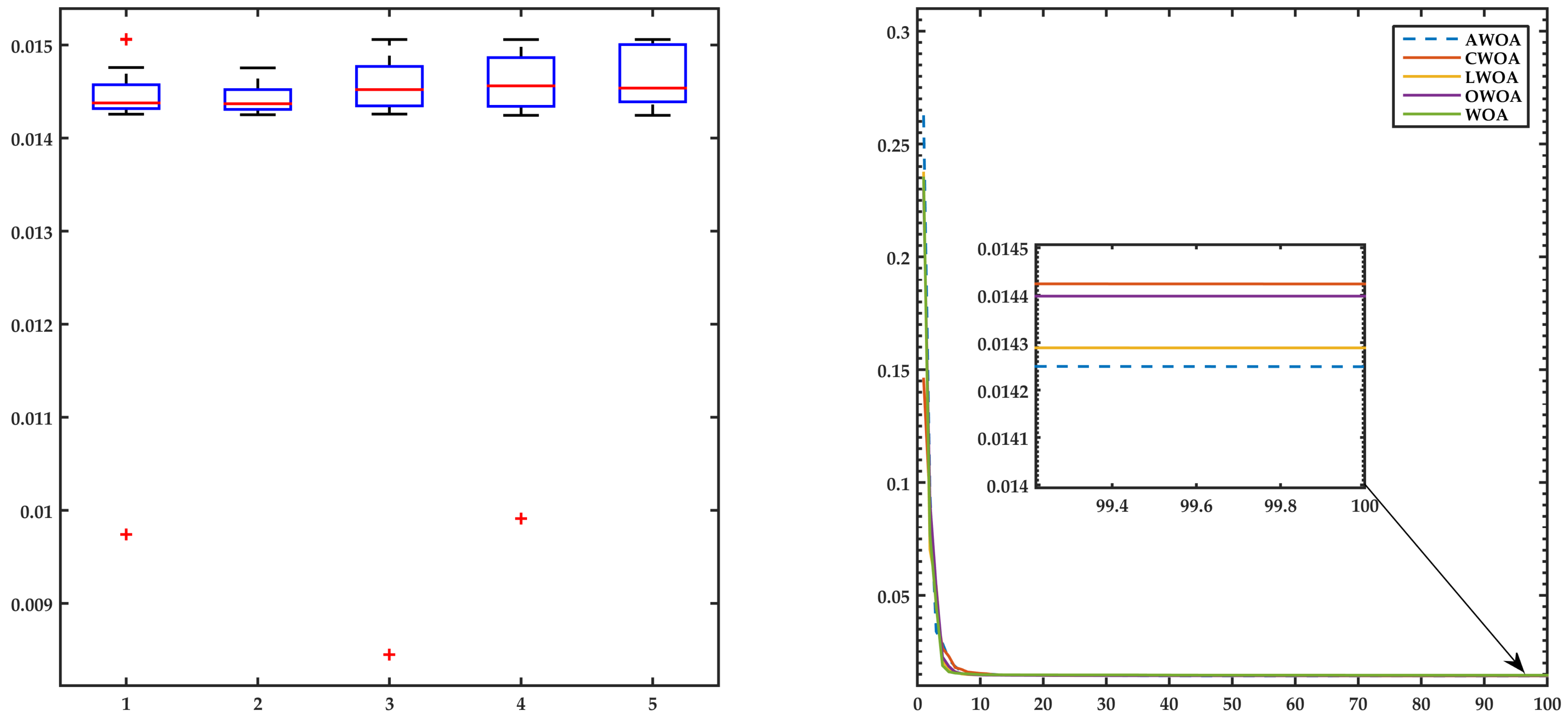
5.1.3. Boxplot Analysis

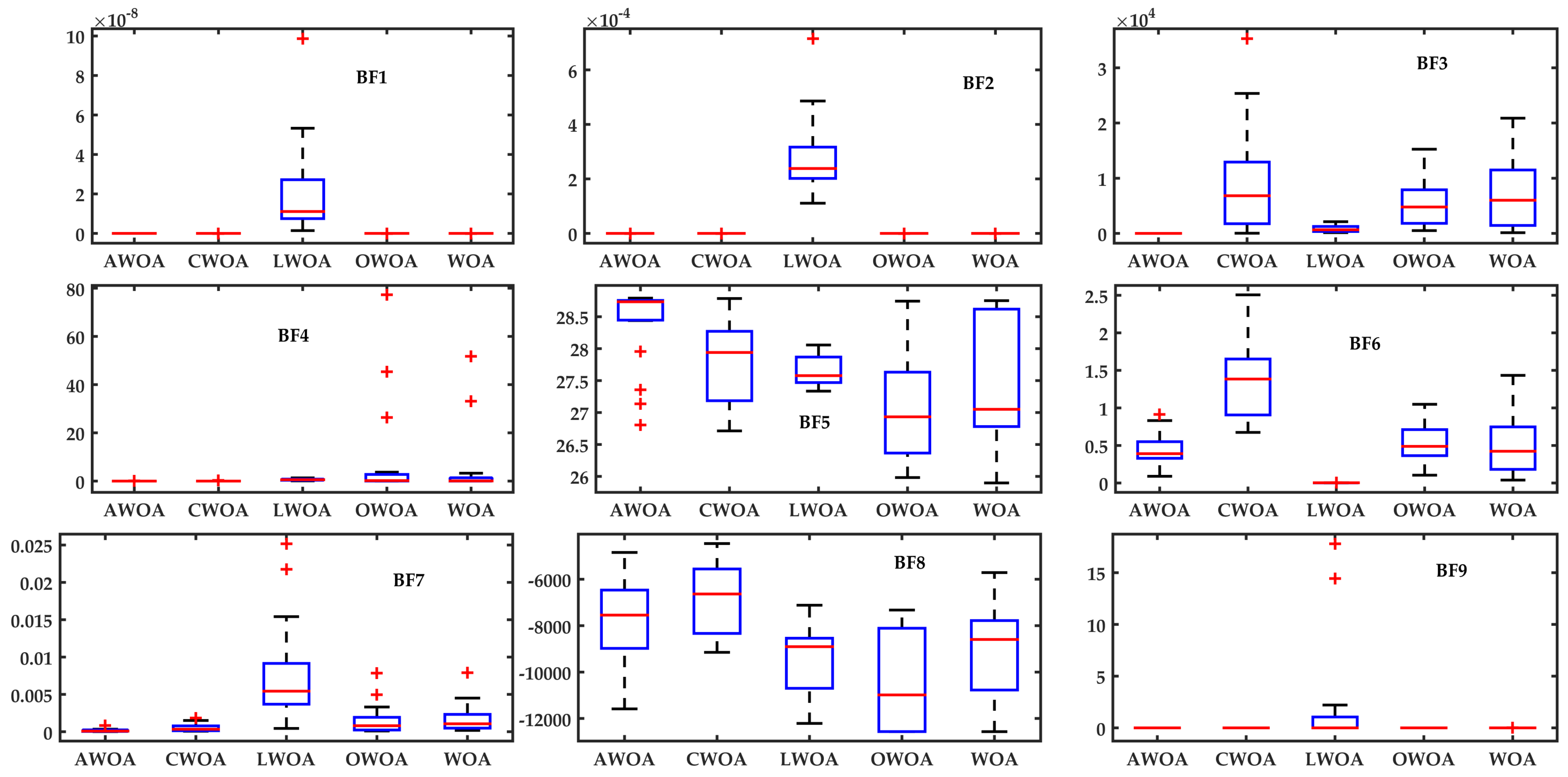
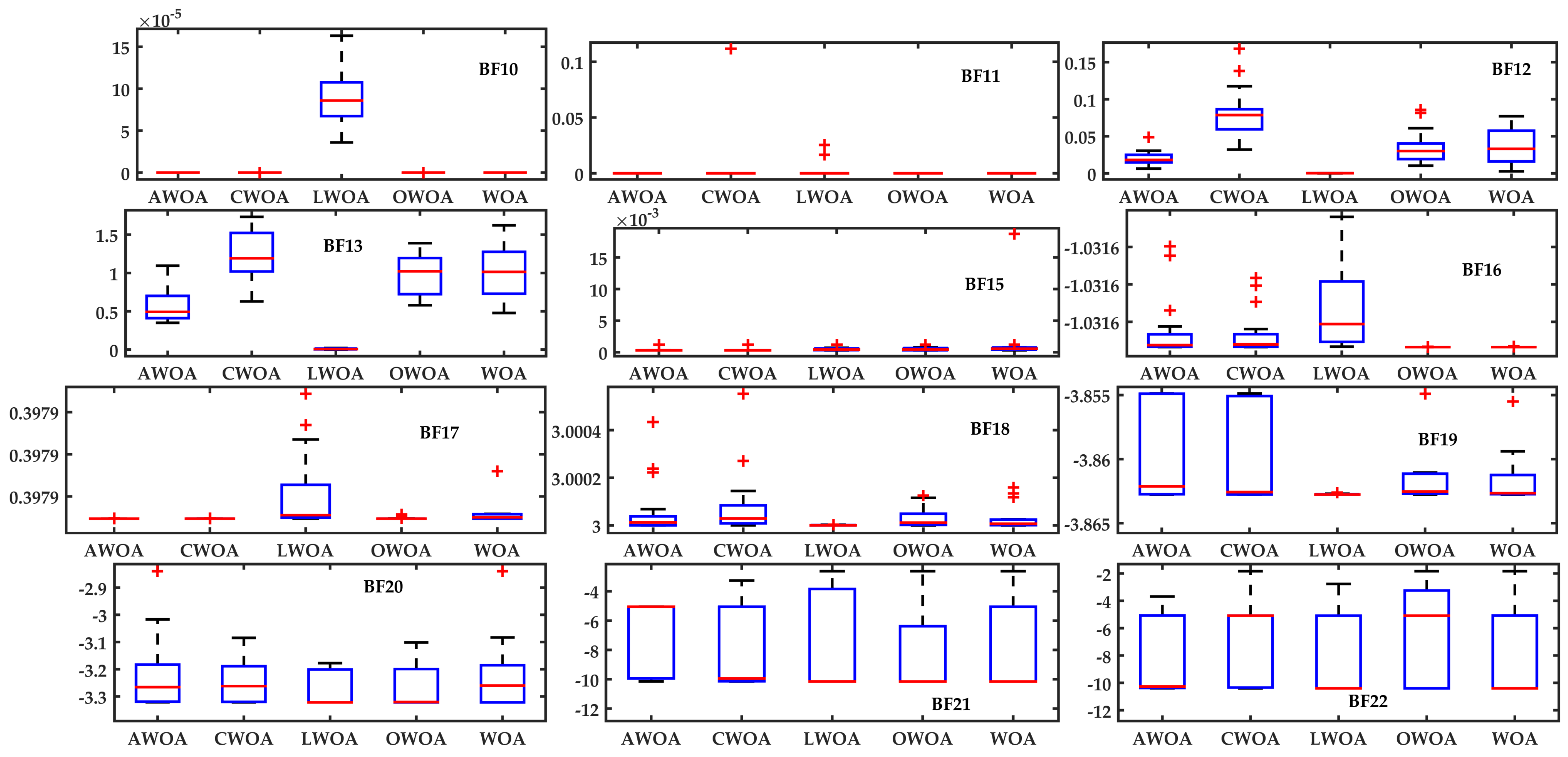
To present a fair comparison between these two opponents, we have plotted boxplots and convergence of some selected functions. Figure 7 shows the boxplots of function (BF1–BF12). From the boxplots, it is observed that the width of the boxplots of AWOA are optimal in these cases; hence, it can be concluded that the optimization performance of AWOA is competitive with other variants of WOA. The mean values shown in the boxplots are also optimal for these functions. The performance of AWOA on the remaining functions of this suite has been depicted through boxplots shown in Figure 8. From these, it can be concluded that the performance of proposed AWOA is competitive, as mean values depicted in the plots are optimal for most of the functions.

5.2. Benchmark Suite 2

In this section, we report the results of the proposed variant on CEC17 functions. The details of CEC 17 functions have been exhibited in Table 2. To check the applicability of the proposed variant on higher as well as lower dimension functions, 10- and 30-dimension problems are chosen deliberately. While performing the simulations we have obeyed the criterion of CEC17; for example, the number of function evaluations have been kept ${10}^4\times D$ for AWOA and other competitors. The results are averaged over 51 independent runs, as indicated by CEC guidelines. The results of the optimization are expressed as mean and standard deviation of the objective function values obtained from the independent runs.

Table 5. Results of Benchmark Suite-2 (10D).

Function	Parameter	WOA	OWOA	AWOA	LWOA	CWOA
F1	Mean	6.85 $\times {10}^4$	7.03 $\times {10}^6$	9.50$\times {\mathbf{10}}^{\mathbf{3}}$	1.48 $\times {10}^7$	1.08 $\times {10}^7$
	SD	1.43 $\times {10}^5$	4.97 $\times {10}^7$	5.84$\times {\mathbf{10}}^{\mathbf{3}}$	5.32 $\times {10}^7$	3.97 $\times {10}^7$
F3	Mean	6.81 $\times {10}^2$	8.53 $\times {10}^2$	3.00$\times {\mathbf{10}}^{\mathbf{2}}$	9.30 $\times {10}^2$	6.17 $\times {10}^2$
	SD	7.92 $\times {10}^2$	1.15 $\times {10}^3$	2.43$\times {\mathbf{10}}^{\mathbf{2}}$	1.15 $\times {10}^3$	5.82 $\times {10}^2$
F4	Mean	4.20 $\times {10}^2$	4.23 $\times {10}^2$	4.05$\times {\mathbf{10}}^{\mathbf{2}}$	4.31 $\times {10}^2$	4.29 $\times {10}^2$
	SD	2.83 $\times 10$	3.16 $\times 10$	1.33$\times \mathbf{10}$	4.11 $\times 10$	3.56 $\times 10$
F5	Mean	5.40 $\times {10}^2$	5.36 $\times {10}^2$	5.28$\times {\mathbf{10}}^{\mathbf{2}}$	5.34 $\times {10}^2$	5.33 $\times {10}^2$
	SD	1.68 $\times 10$	1.57 $\times 10$	9.68	1.04 $\times 10$	1.55 $\times {10}^2$
F6	Mean	6.14 $\times {10}^2$	6.16 $\times {10}^2$	6.03$\times {\mathbf{10}}^{\mathbf{2}}$	6.12 $\times {10}^2$	6.11 $\times {10}^2$
	SD	7.96	7.89	5.00	6.04	5.65
F7	Mean	7.59 $\times {10}^2$	7.61 $\times {10}^2$	7.45$\times {\mathbf{10}}^{\mathbf{2}}$	7.63 $\times {10}^2$	7.51 $\times {10}^2$
	SD	1.64 $\times 10$	1.88 $\times 10$	1.22$\times \mathbf{10}$	1.50 $\times 10$	1.54 $\times 10$
F8	Mean	8.32 $\times {10}^2$	8.31 $\times {10}^2$	8.27$\times {\mathbf{10}}^{\mathbf{2}}$	8.29 $\times {10}^2$	8.29 $\times {10}^2$
	SD	1.08 $\times 10$	1.13 $\times 10$	1.11$\times \mathbf{10}$	1.03 $\times 10$	1.10 $\times 10$
F9	Mean	1.03 $\times {10}^3$	1.04 $\times {10}^3$	9.15$\times {\mathbf{10}}^{\mathbf{2}}$	9.99 $\times {10}^2$	9.88 $\times {10}^2$
	SD	1.11 $\times {10}^2$	1.71 $\times {10}^2$	3.97$\times \mathbf{10}$	9.15 $\times 10$	1.05 $\times {10}^2$
F10	Mean	1.99 $\times {10}^3$	1.94 $\times {10}^3$	1.81$\times {\mathbf{10}}^{\mathbf{3}}$	1.94 $\times {10}^3$	1.84 $\times {10}^3$
	SD	2.87 $\times {10}^2$	3.38 $\times {10}^2$	3.12$\times {\mathbf{10}}^{\mathbf{2}}$	3.41 $\times {10}^2$	2.72 $\times {10}^2$
F11	Mean	1.16 $\times {10}^3$	1.16 $\times {10}^3$	1.13$\times {\mathbf{10}}^{\mathbf{3}}$	1.17 $\times {10}^3$	1.17 $\times {10}^3$
	SD	6.27 $\times 10$	5.89 $\times 10$	1.14$\times \mathbf{10}$	4.84 $\times 10$	6.47 $\times 10$
F12	Mean	1.96 $\times {10}^6$	1.03 $\times {10}^6$	5.29$\times {\mathbf{10}}^{\mathbf{4}}$	2.59 $\times {10}^6$	2.19 $\times {10}^6$
	SD	2.41 $\times {10}^6$	1.82 $\times {10}^6$	5.19$\times {\mathbf{10}}^{\mathbf{4}}$	2.90 $\times {10}^6$	2.25 $\times {10}^6$
F13	Mean	1.66 $\times {10}^4$	1.21 $\times {10}^4$	1.02$\times {\mathbf{10}}^{\mathbf{4}}$	1.91 $\times {10}^4$	1.54 $\times {10}^4$
	SD	1.31 $\times {10}^4$	9.71 $\times {10}^3$	8.32$\times {\mathbf{10}}^{\mathbf{3}}$	1.38 $\times {10}^4$	1.21 $\times {10}^4$
F14	Mean	1.71 $\times {10}^3$	1.71 $\times {10}^3$	1.47$\times {\mathbf{10}}^{\mathbf{3}}$	1.64 $\times {10}^3$	1.70 $\times {10}^3$
	SD	8.69 $\times {10}^2$	8.71 $\times {10}^2$	3.13$\times \mathbf{10}$	6.95 $\times {10}^2$	7.96 $\times {10}^2$
F15	Mean	2.41 $\times {10}^3$	2.81 $\times {10}^3$	1.58$\times {\mathbf{10}}^{\mathbf{3}}$	2.64 $\times {10}^3$	2.58 $\times {10}^3$
	SD	1.17 $\times {10}^3$	1.41 $\times {10}^3$	4.47$\times \mathbf{10}$	1.30 $\times {10}^3$	1.22 $\times {10}^3$
F16	Mean	1.76 $\times {10}^3$	1.78 $\times {10}^3$	1.76 $\times {10}^3$	1.78 $\times {10}^3$	1.73$\times {\mathbf{10}}^{\mathbf{3}}$
	SD	1.22 $\times {10}^2$	1.25 $\times {10}^2$	1.37 $\times {10}^2$	1.01 $\times {10}^2$	9.82$\times \mathbf{10}$
F17	Mean	1.77 $\times {10}^3$	1.77 $\times {10}^3$	1.77 $\times {10}^3$	1.76$\times {\mathbf{10}}^{\mathbf{3}}$	1.77 $\times {10}^3$
	SD	3.23 $\times 10$	3.60 $\times 10$	3.16 $\times 10$	2.46$\times \mathbf{10}$	3.08 $\times 10$
F18	Mean	1.70 $\times {10}^4$	1.71 $\times {10}^4$	1.72 $\times {10}^4$	1.62$\times {\mathbf{10}}^{\mathbf{4}}$	1.62 $\times {10}^4$
	SD	1.24 $\times {10}^4$	1.14 $\times {10}^4$	1.02 $\times {10}^4$	1.20$\times {\mathbf{10}}^{\mathbf{4}}$	1.07 $\times {10}^4$
F19	Mean	8.18 $\times {10}^3$	1.69 $\times {10}^4$	2.32$\times {\mathbf{10}}^{\mathbf{3}}$	4.93 $\times {10}^3$	5.40 $\times {10}^3$
	SD	6.91 $\times {10}^3$	5.21 $\times {10}^4$	6.54$\times {\mathbf{10}}^{\mathbf{2}}$	5.01 $\times {10}^3$	5.25 $\times {10}^3$
F20	Mean	2.09 $\times {10}^3$	2.10 $\times {10}^3$	2.05$\times {\mathbf{10}}^{\mathbf{3}}$	2.11 $\times {10}^3$	2.11 $\times {10}^3$
	SD	5.62 $\times 10$	5.21 $\times 10$	4.18$\times \mathbf{10}$	5.48 $\times 10$	5.48 $\times 10$
F21	Mean	2.31 $\times {10}^3$	2.31 $\times {10}^3$	2.30 $\times {10}^3$	2.27$\times {\mathbf{10}}^{\mathbf{3}}$	2.29 $\times {10}^3$
	SD	5.97 $\times 10$	5.40 $\times 10$	6.20 $\times 10$	6.29$\times \mathbf{10}$	5.86 $\times 10$
F22	Mean	2.33 $\times {10}^3$	2.31 $\times {10}^3$	2.30$\times {\mathbf{10}}^{\mathbf{3}}$	2.31 $\times {10}^3$	2.31 $\times {10}^3$
	SD	1.63 $\times {10}^2$	9.37	1.63$\times \mathbf{10}$	2.19 $\times 10$	7.34
F23	Mean	2.64 $\times {10}^3$	2.64 $\times {10}^3$	2.64 $\times {10}^3$	2.63$\times {\mathbf{10}}^{\mathbf{3}}$	2.64 $\times {10}^3$
	SD	1.80 $\times 10$	1.46 $\times 10$	1.44 $\times 10$	1.11$\times \mathbf{10}$	1.41 $\times 10$
F24	Mean	2.75 $\times {10}^3$	2.76 $\times {10}^3$	2.75 $\times {10}^3$	2.75 $\times {10}^3$	2.74$\times {\mathbf{10}}^{\mathbf{3}}$
	SD	8.30 $\times 10$	5.41 $\times 10$	7.43 $\times 10$	5.89 $\times 10$	7.11$\times \mathbf{10}$
F25	Mean	2.94 $\times {10}^3$	2.93 $\times {10}^3$	2.92$\times {\mathbf{10}}^{\mathbf{3}}$	2.94 $\times {10}^3$	2.93 $\times {10}^3$
	SD	4.61 $\times 10$	4.91 $\times 10$	5.31$\times \mathbf{10}$	2.03 $\times 10$	4.42 $\times 10$
F26	Mean	3.22 $\times {10}^3$	3.13 $\times {10}^3$	3.04 $\times {10}^3$	3.03$\times {\mathbf{10}}^{\mathbf{3}}$	3.03 $\times {10}^3$
	SD	3.78 $\times {10}^2$	2.83 $\times {10}^2$	2.54 $\times {10}^2$	1.75$\times {\mathbf{10}}^{\mathbf{2}}$	1.87 $\times {10}^2$
F27	Mean	3.12 $\times {10}^3$	3.11 $\times {10}^3$	3.11$\times {\mathbf{10}}^{\mathbf{3}}$	3.11 $\times {10}^3$	3.11 $\times {10}^3$
	SD	2.86 $\times 10$	2.62 $\times 10$	2.61$\times \mathbf{10}$	2.79 $\times 10$	2.21 $\times 10$
F28	Mean	3.33 $\times {10}^3$	3.31 $\times {10}^3$	3.30$\times {\mathbf{10}}^{\mathbf{3}}$	3.33 $\times {10}^3$	3.33 $\times {10}^3$
	SD	1.51 $\times {10}^2$	1.47 $\times {10}^2$	1.48$\times {\mathbf{10}}^{\mathbf{2}}$	1.11 $\times {10}^2$	1.36 $\times {10}^2$
F29	Mean	3.27 $\times {10}^3$	3.27 $\times {10}^3$	3.24 $\times {10}^3$	3.23$\times {\mathbf{10}}^{\mathbf{2}}$	3.25 $\times {10}^3$
	SD	6.70 $\times 10$	6.43 $\times 10$	5.72 $\times 10$	5.74$\times \mathbf{10}$	6.53 $\times 10$
F30	Mean	2.19 $\times {10}^5$	3.56 $\times {10}^5$	9.26$\times {\mathbf{10}}^{\mathbf{4}}$	1.37 $\times {10}^5$	2.36 $\times {10}^5$
	SD	3.74 $\times {10}^5$	5.50 $\times {10}^5$	2.82$\times {\mathbf{10}}^{\mathbf{5}}$	3.16 $\times {10}^5$	4.30 $\times {10}^5$

and

Table 6. Results of Benchmark Suite-2 (30D).

Function	Parameter	WOA	OWOA	AWOA	LWOA	CWOA
F1	Mean	1.35 $\times {10}^9$	1.61 $\times {10}^9$	4.53$\times {\mathbf{10}}^{\mathbf{5}}$	2.36 $\times {10}^9$	2.65 $\times {10}^9$
	SD	1.23 $\times {10}^9$	2.06 $\times {10}^9$	1.71$\times {\mathbf{10}}^{\mathbf{5}}$	1.64 $\times {10}^9$	1.50 $\times {10}^9$
F3	Mean	4.85 $\times {10}^4$	4.78 $\times {10}^4$	3.24$\times {\mathbf{10}}^{\mathbf{2}}$	4.83 $\times {10}^4$	4.57 $\times {10}^4$
	SD	1.53 $\times {10}^4$	1.34 $\times {10}^4$	6.57	7.64 $\times {10}^3$	1.14 $\times {10}^4$
F4	Mean	5.93 $\times {10}^2$	6.05 $\times {10}^2$	4.95$\times {\mathbf{10}}^{\mathbf{2}}$	7.73 $\times {10}^2$	7.48 $\times {10}^2$
	SD	6.03 $\times 10$	7.17 $\times 10$	2.29$\times \mathbf{10}$	1.81 $\times {10}^2$	1.40 $\times {10}^2$
F5	Mean	7.60 $\times {10}^2$	7.67 $\times {10}^2$	7.13$\times {\mathbf{10}}^{\mathbf{2}}$	7.68 $\times {10}^2$	7.52 $\times {10}^2$
	SD	5.98 $\times 10$	5.95 $\times 10$	5.24$\times \mathbf{10}$	4.44 $\times 10$	4.98 $\times 10$
F6	Mean	6.66 $\times {10}^2$	6.65 $\times {10}^2$	6.51$\times {\mathbf{10}}^{\mathbf{2}}$	6.58 $\times {10}^2$	6.58 $\times {10}^2$
	SD	1.21 $\times 10$	1.06 $\times 10$	9.99	1.00 $\times 10$	9.64
F7	Mean	1.18 $\times {10}^3$	1.16 $\times {10}^3$	1.09$\times {\mathbf{10}}^{\mathbf{3}}$	1.15 $\times {10}^3$	1.14 $\times {10}^3$
	SD	1.09 $\times {10}^2$	8.42 $\times 10$	9.02$\times \mathbf{10}$	8.04 $\times 10$	6.47 $\times 10$
F8	Mean	1.01 $\times {10}^3$	1.01 $\times {10}^3$	9.80$\times {\mathbf{10}}^{\mathbf{2}}$	1.01 $\times {10}^3$	1.00 $\times {10}^3$
	SD	4.78 $\times 10$	4.62 $\times 10$	4.87$\times \mathbf{10}$	2.94 $\times 10$	4.26 $\times 10$
F9	Mean	7.31 $\times {10}^3$	7.61 $\times {10}^3$	6.48$\times {\mathbf{10}}^{\mathbf{3}}$	6.58 $\times {10}^3$	6.74 $\times {10}^3$
	SD	2.91 $\times {10}^3$	2.61 $\times {10}^3$	2.08$\times {\mathbf{10}}^{\mathbf{3}}$	1.64 $\times {10}^3$	2.04 $\times {10}^3$
F10	Mean	5.93 $\times {10}^3$	6.06 $\times {10}^3$	4.98$\times {\mathbf{10}}^{\mathbf{3}}$	6.81 $\times {10}^3$	6.42 $\times {10}^3$
	SD	7.21 $\times {10}^2$	6.72 $\times {10}^2$	6.81$\times {\mathbf{10}}^{\mathbf{2}}$	7.10 $\times {10}^2$	8.61 $\times {10}^2$
F11	Mean	2.09 $\times {10}^3$	1.80 $\times {10}^3$	1.27$\times {\mathbf{10}}^{\mathbf{3}}$	1.94 $\times {10}^3$	2.08 $\times {10}^3$
	SD	9.83 $\times {10}^2$	7.53 $\times {10}^2$	5.97$\times \mathbf{10}$	5.86 $\times {10}^2$	6.85 $\times {10}^2$
F12	Mean	5.19 $\times {10}^7$	5.45 $\times {10}^7$	4.36$\times {\mathbf{10}}^{\mathbf{6}}$	2.38 $\times {10}^8$	1.76 $\times {10}^8$
	SD	5.05 $\times {10}^7$	4.00 $\times {10}^7$	2.82$\times {\mathbf{10}}^{\mathbf{6}}$	2.39 $\times {10}^8$	1.25 $\times {10}^8$
F13	Mean	2.60 $\times {10}^5$	1.58 $\times {10}^5$	1.46$\times {\mathbf{10}}^{\mathbf{5}}$	7.88 $\times {10}^6$	2.13 $\times {10}^6$
	SD	7.92 $\times {10}^5$	1.75 $\times {10}^5$	1.05$\times {\mathbf{10}}^{\mathbf{5}}$	2.55 $\times {10}^5$	1.10 $\times {10}^7$
F14	Mean	4.41 $\times {10}^5$	3.52 $\times {10}^5$	2.46$\times {\mathbf{10}}^{\mathbf{4}}$	4.22 $\times {10}^5$	4.79 $\times {10}^5$
	SD	7.29 $\times {10}^2$	4.31 $\times {10}^5$	1.56$\times {\mathbf{10}}^{\mathbf{4}}$	4.92 $\times {10}^5$	5.11 $\times {10}^5$
F15	Mean	2.78 $\times {10}^5$	2.51 $\times {10}^6$	7.96$\times {\mathbf{10}}^{\mathbf{4}}$	1.67 $\times {10}^6$	4.31 $\times {10}^6$
	SD	5.75 $\times {10}^5$	9.42 $\times {10}^6$	4.71$\times {\mathbf{10}}^{\mathbf{4}}$	2.63 $\times {10}^6$	9.62 $\times {10}^6$
F16	Mean	3.22 $\times {10}^3$	3.25 $\times {10}^3$	2.87$\times {\mathbf{10}}^{\mathbf{3}}$	3.42 $\times {10}^3$	3.43 $\times {10}^3$
	SD	3.71 $\times {10}^2$	4.08 $\times {10}^2$	3.13$\times {\mathbf{10}}^{\mathbf{2}}$	3.97 $\times {10}^2$	3.65 $\times {10}^2$
F17	Mean	2.42 $\times {10}^3$	2.42 $\times {10}^3$	2.37$\times {\mathbf{10}}^{\mathbf{3}}$	2.41 $\times {10}^3$	2.42 $\times {10}^3$
	SD	2.33 $\times {10}^2$	2.43 $\times {10}^2$	2.62$\times {\mathbf{10}}^{\mathbf{2}}$	1.97 $\times {10}^2$	1.81 $\times {10}^2$
F18	Mean	1.74 $\times {10}^6$	2.30 $\times {10}^6$	2.29$\times {\mathbf{10}}^{\mathbf{5}}$	4.18 $\times {10}^6$	2.74 $\times {10}^6$
	SD	1.77 $\times {10}^6$	2.52 $\times {10}^6$	1.89$\times {\mathbf{10}}^{\mathbf{5}}$	3.89 $\times {10}^6$	2.57 $\times {10}^6$
F19	Mean	1.78 $\times {10}^6$	2.25 $\times {10}^6$	1.22$\times {\mathbf{10}}^{\mathbf{5}}$	7.62 $\times {10}^6$	6.83 $\times {10}^6$
	SD	1.64 $\times {10}^6$	2.01 $\times {10}^6$	7.15$\times {\mathbf{10}}^{\mathbf{4}}$	5.58 $\times {10}^6$	1.12 $\times {10}^7$
F20	Mean	2.69 $\times {10}^3$	2.67 $\times {10}^3$	2.60$\times {\mathbf{10}}^{\mathbf{3}}$	2.67 $\times {10}^3$	2.67 $\times {10}^3$
	SD	1.99 $\times {10}^2$	1.81 $\times {10}^2$	2.11$\times {\mathbf{10}}^{\mathbf{2}}$	1.70 $\times {10}^2$	2.02 $\times {10}^2$
F21	Mean	2.54 $\times {10}^3$	2.53 $\times {10}^3$	2.51$\times {\mathbf{10}}^{\mathbf{3}}$	2.53 $\times {10}^3$	2.53 $\times {10}^3$
	SD	5.43 $\times 10$	5.18 $\times 10$	4.98$\times {\mathbf{10}}^{\mathbf{3}}$	4.82 $\times 10$	4.72 $\times 10$
F22	Mean	6.51 $\times {10}^3$	6.39 $\times {10}^3$	5.69$\times {\mathbf{10}}^{\mathbf{3}}$	6.19 $\times {10}^3$	7.42 $\times {10}^3$
	SD	2.08 $\times {10}^3$	1.93 $\times {10}^3$	1.90$\times {\mathbf{10}}^{\mathbf{3}}$	2.46 $\times {10}^3$	1.59 $\times {10}^3$
F23	Mean	2.97 $\times {10}^3$	2.97 $\times {10}^3$	2.93$\times {\mathbf{10}}^{\mathbf{3}}$	2.94 $\times {10}^3$	2.94 $\times {10}^3$
	SD	8.35 $\times 10$	7.33 $\times 10$	8.35$\times \mathbf{10}$	6.26 $\times 10$	5.59 $\times 10$
F24	Mean	3.12 $\times {10}^3$	3.10 $\times {10}^3$	3.15 $\times {10}^3$	3.09 $\times {10}^3$	3.08$\times {\mathbf{10}}^{\mathbf{3}}$
	SD	7.23 $\times 10$	7.51 $\times 10$	8.51 $\times 10$	5.79 $\times 10$	4.63$\times \mathbf{10}$
F25	Mean	3.01 $\times {10}^3$	3.00 $\times {10}^3$	2.89$\times {\mathbf{10}}^{\mathbf{3}}$	3.07 $\times {10}^3$	3.05 $\times {10}^3$
	SD	5.54 $\times 10$	5.79 $\times 10$	1.62$\times \mathbf{10}$	4.41 $\times 10$	4.56 $\times 10$
F26	Mean	6.63 $\times {10}^3$	6.94 $\times {10}^3$	6.12$\times {\mathbf{10}}^{\mathbf{3}}$	6.60 $\times {10}^3$	6.56 $\times {10}^3$
	SD	9.57 $\times {10}^2$	8.47 $\times {10}^2$	1.12$\times {\mathbf{10}}^{\mathbf{3}}$	8.13 $\times {10}^2$	8.41 $\times {10}^2$
F27	Mean	3.32 $\times {10}^3$	3.32 $\times {10}^3$	3.27$\times {\mathbf{10}}^{\mathbf{3}}$	3.37 $\times {10}^3$	3.35 $\times {10}^3$
	SD	4.56 $\times 10$	5.12 $\times 10$	4.04$\times \mathbf{10}$	6.38 $\times 10$	6.36 $\times 10$
F28	Mean	3.40 $\times {10}^3$	3.42 $\times {10}^3$	3.22$\times {\mathbf{10}}^{\mathbf{3}}$	3.50 $\times {10}^3$	3.50 $\times {10}^3$
	SD	7.82 $\times 10$	8.98 $\times 10$	2.20$\times \mathbf{10}$	1.13 $\times {10}^2$	9.80 $\times 10$
F29	Mean	4.63 $\times {10}^3$	4.58 $\times {10}^3$	4.06$\times {\mathbf{10}}^{\mathbf{3}}$	4.67 $\times {10}^3$	4.57 $\times {10}^3$
	SD	3.07 $\times {10}^2$	3.11 $\times {10}^2$	2.77$\times {\mathbf{10}}^{\mathbf{2}}$	3.56 $\times {10}^2$	3.82 $\times {10}^2$
F30	Mean	8.90 $\times {10}^6$	9.96 $\times {10}^6$	4.28$\times {\mathbf{10}}^{\mathbf{5}}$	2.54 $\times {10}^7$	2.38 $\times {10}^7$
	SD	5.90 $\times {10}^6$	6.80 $\times {10}^6$	1.92$\times {\mathbf{10}}^{\mathbf{5}}$	2.30 $\times {10}^7$	1.83 $\times {10}^7$

show these analyses and the bold face entries in the tables show the best performer.

Table 7. Results of the rank sum test on Benchmark Suite-2 (10D).

Function	WOA	OWOA	LWOA	CWOA
F1	2.58 $\times {10}^{-1}$	3.99 $\times {10}^{-1}$	3.30 $\times {10}^{-18}$	3.30 $\times {10}^{-18}$
F3	3.30$\times {\mathbf{10}}^{-\mathbf{18}}$	3.30$\times {\mathbf{10}}^{-\mathbf{18}}$	3.30$\times {\mathbf{10}}^{-\mathbf{18}}$	3.30$\times {\mathbf{10}}^{-\mathbf{18}}$
F4	4.20$\times {\mathbf{10}}^{-\mathbf{9}}$	2.99$\times {\mathbf{10}}^{-\mathbf{13}}$	3.00$\times {\mathbf{10}}^{-\mathbf{15}}$	4.73$\times {\mathbf{10}}^{-\mathbf{16}}$
F5	1.40$\times {\mathbf{10}}^{-\mathbf{4}}$	1.08$\times {\mathbf{10}}^{-\mathbf{2}}$	3.92$\times {\mathbf{10}}^{-\mathbf{3}}$	9.97$\times {\mathbf{10}}^{-\mathbf{2}}$
F6	1.56$\times {\mathbf{10}}^{-\mathbf{13}}$	5.13$\times {\mathbf{10}}^{-\mathbf{15}}$	6.26$\times {\mathbf{10}}^{-\mathbf{13}}$	9.11$\times {\mathbf{10}}^{-\mathbf{12}}$
F7	8.04 $\times {10}^{-6}$	1.73 $\times {10}^{-5}$	1.23 $\times {10}^{-8}$	3.99 $\times {10}^{-2}$
F8	3.22 $\times {10}^{-2}$	1.29 $\times {10}^{-1}$	3.15 $\times {10}^{-1}$	4.45 $\times {10}^{-1}$
F9	2.57 $\times {10}^{-13}$	4.90 $\times {10}^{-13}$	8.00 $\times {10}^{-13}$	4.51 $\times {10}^{-12}$
F10	5.59 $\times {10}^{-3}$	5.15 $\times {10}^{-2}$	5.73 $\times {10}^{-2}$	4.70 $\times {10}^{-1}$
F11	1.35 $\times {10}^{-3}$	1.56 $\times {10}^{-4}$	4.44 $\times {10}^{-10}$	1.32 $\times {10}^{-10}$
F12	1.47$\times {\mathbf{10}}^{-\mathbf{14}}$	2.33$\times {\mathbf{10}}^{-\mathbf{10}}$	2.33$\times {\mathbf{10}}^{-\mathbf{13}}$	1.74$\times {\mathbf{10}}^{-\mathbf{12}}$
F13	4.94$\times {\mathbf{10}}^{-\mathbf{3}}$	2.90 $\times {10}^{-1}$	9.03$\times {\mathbf{10}}^{-\mathbf{5}}$	1.06$\times {\mathbf{10}}^{-\mathbf{2}}$
F14	4.09$\times {\mathbf{10}}^{-\mathbf{3}}$	1.02$\times {\mathbf{10}}^{-\mathbf{3}}$	4.20$\times {\mathbf{10}}^{-\mathbf{4}}$	2.34 $\times {10}^{-1}$
F15	9.26$\times {\mathbf{10}}^{-\mathbf{13}}$	5.40$\times {\mathbf{10}}^{-\mathbf{13}}$	3.17$\times {\mathbf{10}}^{-\mathbf{15}}$	1.66$\times {\mathbf{10}}^{-\mathbf{15}}$
F16	6.02 $\times {10}^{-1}$	1.72 $\times {10}^{-1}$	8.30 $\times {10}^{-2}$	6.06 $\times {10}^{-1}$
F17	5.38 $\times {10}^{-1}$	2.18 $\times {10}^{-1}$	7.89 $\times {10}^{-1}$	4.66 $\times {10}^{-1}$
F18	5.83 $\times {10}^{-1}$	8.30 $\times {10}^{-1}$	3.73 $\times {10}^{-1}$	5.47 $\times {10}^{-1}$
F19	2.47 $\times {10}^{-8}$	5.71 $\times {10}^{-8}$	2.61 $\times {10}^{-1}$	6.57 $\times {10}^{-2}$
F20	1.20 $\times {10}^{-5}$	1.14 $\times {10}^{-6}$	2.47 $\times {10}^{-7}$	4.22 $\times {10}^{-8}$
F21	7.39 $\times {10}^{-2}$	2.55 $\times {10}^{-1}$	2.21 $\times {10}^{-1}$	2.50 $\times {10}^{-1}$
F22	1.60$\times {\mathbf{10}}^{-\mathbf{6}}$	6.88$\times {\mathbf{10}}^{-\mathbf{6}}$	6.60$\times {\mathbf{10}}^{-\mathbf{7}}$	9.26$\times {\mathbf{10}}^{-\mathbf{11}}$
F23	5.37$\times {\mathbf{10}}^{-\mathbf{3}}$	5.73 $\times {10}^{-2}$	8.36 $\times {10}^{-1}$	1.29 $\times {10}^{-1}$
F24	6.83 $\times {10}^{-1}$	2.87 $\times {10}^{-1}$	1.08 $\times {10}^{-1}$	1.54 $\times {10}^{-2}$
F25	2.01$\times {\mathbf{10}}^{-\mathbf{5}}$	3.43$\times {\mathbf{10}}^{-\mathbf{4}}$	1.32$\times {\mathbf{10}}^{-\mathbf{3}}$	1.02$\times {\mathbf{10}}^{-\mathbf{2}}$
F26	1.17$\times {\mathbf{10}}^{-\mathbf{3}}$	2.60$\times {\mathbf{10}}^{-\mathbf{3}}$	1.43 $\times {10}^{-1}$	3.00 $\times {10}^{-1}$
F27	2.58$\times {\mathbf{10}}^{-\mathbf{2}}$	3.17$\times {\mathbf{10}}^{-\mathbf{2}}$	1.30 $\times {10}^{-1}$	9.83 $\times {10}^{-2}$
F28	6.06 $\times {10}^{-1}$	3.32 $\times {10}^{-1}$	1.29$\times {\mathbf{10}}^{-\mathbf{3}}$	2.54$\times {\mathbf{10}}^{-\mathbf{3}}$
F29	4.68$\times {\mathbf{10}}^{-\mathbf{2}}$	3.22$\times {\mathbf{10}}^{-\mathbf{2}}$	2.47 $\times {10}^{-1}$	9.25 $\times {10}^{-1}$
F30	4.70$\times {\mathbf{10}}^{-\mathbf{6}}$	1.49$\times {\mathbf{10}}^{-\mathbf{5}}$	2.23$\times {\mathbf{10}}^{-\mathbf{6}}$	1.65$\times {\mathbf{10}}^{-\mathbf{6}}$

and

Table 8. Results of the rank sum test on Benchmark Suite-2 (30D).

Function	WOA	OWOA	LWOA	CWOA
F1	3.30$\times {\mathbf{10}}^{-\mathbf{18}}$	3.30$\times {\mathbf{10}}^{-\mathbf{18}}$	3.30$\times {\mathbf{10}}^{-\mathbf{18}}$	3.30$\times {\mathbf{10}}^{-\mathbf{18}}$
F3	3.30$\times {\mathbf{10}}^{-\mathbf{18}}$	3.30$\times {\mathbf{10}}^{-\mathbf{18}}$	3.30$\times {\mathbf{10}}^{-\mathbf{18}}$	3.30$\times {\mathbf{10}}^{-\mathbf{18}}$
F4	1.05$\times {\mathbf{10}}^{-\mathbf{16}}$	1.39$\times {\mathbf{10}}^{-\mathbf{16}}$	3.30$\times {\mathbf{10}}^{-\mathbf{18}}$	3.30$\times {\mathbf{10}}^{-\mathbf{18}}$
F5	1.13$\times {\mathbf{10}}^{-\mathbf{4}}$	1.06$\times {\mathbf{10}}^{-\mathbf{5}}$	7.07$\times {\mathbf{10}}^{-\mathbf{7}}$	3.17$\times {\mathbf{10}}^{-\mathbf{4}}$
F6	6.03$\times {\mathbf{10}}^{-\mathbf{9}}$	5.14$\times {\mathbf{10}}^{-\mathbf{9}}$	7.08$\times {\mathbf{10}}^{-\mathbf{4}}$	1.17$\times {\mathbf{10}}^{-\mathbf{3}}$
F7	3.74$\times {\mathbf{10}}^{-\mathbf{5}}$	3.01$\times {\mathbf{10}}^{-\mathbf{4}}$	8.80$\times {\mathbf{10}}^{-\mathbf{4}}$	3.23$\times {\mathbf{10}}^{-\mathbf{3}}$
F8	2.96$\times {\mathbf{10}}^{-\mathbf{3}}$	3.68$\times {\mathbf{10}}^{-\mathbf{3}}$	3.99$\times {\mathbf{10}}^{-\mathbf{4}}$	1.28 $\times {10}^{-2}$
F9	2.34 $\times {10}^{-1}$	3.17$\times {\mathbf{10}}^{-\mathbf{2}}$	4.66 $\times {10}^{-1}$	4.34 $\times {10}^{-1}$
F10	1.09$\times {\mathbf{10}}^{-\mathbf{8}}$	1.79$\times {\mathbf{10}}^{-\mathbf{10}}$	2.43$\times {\mathbf{10}}^{-\mathbf{16}}$	3.08$\times {\mathbf{10}}^{-\mathbf{12}}$
F11	3.78$\times {\mathbf{10}}^{-\mathbf{17}}$	9.65$\times {\mathbf{10}}^{-\mathbf{16}}$	3.72$\times {\mathbf{10}}^{-\mathbf{18}}$	3.72$\times {\mathbf{10}}^{-\mathbf{18}}$
F12	1.42$\times {\mathbf{10}}^{-\mathbf{17}}$	1.27$\times {\mathbf{10}}^{-\mathbf{17}}$	3.30$\times {\mathbf{10}}^{-\mathbf{18}}$	4.70$\times {\mathbf{10}}^{-\mathbf{18}}$
F13	5.83 $\times {10}^{-1}$	7.53 $\times {10}^{-1}$	1.63$\times {\mathbf{10}}^{-\mathbf{14}}$	2.84$\times {\mathbf{10}}^{-\mathbf{13}}$
F14	2.56$\times {\mathbf{10}}^{-\mathbf{15}}$	1.41$\times {\mathbf{10}}^{-\mathbf{15}}$	8.44$\times {\mathbf{10}}^{-\mathbf{18}}$	5.41$\times {\mathbf{10}}^{-\mathbf{15}}$
F15	7.39 $\times {10}^{-2}$	8.19$\times {\mathbf{10}}^{-\mathbf{4}}$	7.30$\times {\mathbf{10}}^{-\mathbf{14}}$	1.34$\times {\mathbf{10}}^{-\mathbf{13}}$
F16	2.30$\times {\mathbf{10}}^{-\mathbf{6}}$	6.88$\times {\mathbf{10}}^{-\mathbf{6}}$	1.64$\times {\mathbf{10}}^{-\mathbf{9}}$	1.26 $\times {10}^{-10}$
F17	3.29 $\times {10}^{-1}$	4.58 $\times {10}^{-1}$	4.22 $\times {10}^{-1}$	3.00 $\times {10}^{-1}$
F18	4.30$\times {\mathbf{10}}^{-\mathbf{12}}$	1.07$\times {\mathbf{10}}^{-\mathbf{12}}$	3.72$\times {\mathbf{10}}^{-\mathbf{15}}$	4.15$\times {\mathbf{10}}^{-\mathbf{14}}$
F19	1.95$\times {\mathbf{10}}^{-\mathbf{16}}$	1.34$\times {\mathbf{10}}^{-\mathbf{15}}$	3.72$\times {\mathbf{10}}^{-\mathbf{18}}$	1.72$\times {\mathbf{10}}^{-\mathbf{14}}$
F20	3.80$\times {\mathbf{10}}^{-\mathbf{2}}$	9.17 $\times {10}^{-2}$	1.10 $\times {10}^{-1}$	1.30 $\times {10}^{-1}$
F21	3.44$\times {\mathbf{10}}^{-\mathbf{2}}$	1.13 $\times {10}^{-1}$	1.99 $\times {10}^{-1}$	1.45 $\times {10}^{-1}$
F22	5.82$\times {\mathbf{10}}^{-\mathbf{4}}$	1.07$\times {\mathbf{10}}^{-\mathbf{3}}$	5.71$\times {\mathbf{10}}^{-\mathbf{3}}$	5.50$\times {\mathbf{10}}^{-\mathbf{10}}$
F23	8.53$\times {\mathbf{10}}^{-\mathbf{3}}$	9.23$\times {\mathbf{10}}^{-\mathbf{3}}$	4.14 $\times {10}^{-1}$	2.44 $\times {10}^{-1}$
F24	3.86$\times {\mathbf{10}}^{-\mathbf{2}}$	3.30$\times {\mathbf{10}}^{-\mathbf{3}}$	2.26$\times {\mathbf{10}}^{-\mathbf{4}}$	1.58$\times {\mathbf{10}}^{-\mathbf{5}}$
F25	1.27$\times {\mathbf{10}}^{-\mathbf{17}}$	8.44$\times {\mathbf{10}}^{-\mathbf{18}}$	3.30$\times {\mathbf{10}}^{-\mathbf{18}}$	3.30$\times {\mathbf{10}}^{-\mathbf{18}}$
F26	2.67$\times {\mathbf{10}}^{-\mathbf{2}}$	1.56$\times {\mathbf{10}}^{-\mathbf{4}}$	7.72 $\times {10}^{-2}$	4.26$\times {\mathbf{10}}^{-\mathbf{2}}$
F27	1.14$\times {\mathbf{10}}^{-\mathbf{8}}$	6.53$\times {\mathbf{10}}^{-\mathbf{9}}$	4.60$\times {\mathbf{10}}^{-\mathbf{14}}$	3.56$\times {\mathbf{10}}^{-\mathbf{12}}$
F28	5.61$\times {\mathbf{10}}^{-\mathbf{18}}$	3.30$\times {\mathbf{10}}^{-\mathbf{18}}$	3.30$\times {\mathbf{10}}^{-\mathbf{18}}$	3.30$\times {\mathbf{10}}^{-\mathbf{18}}$
F29	3.64$\times {\mathbf{10}}^{-\mathbf{13}}$	5.98$\times {\mathbf{10}}^{-\mathbf{12}}$	9.26$\times {\mathbf{10}}^{-\mathbf{13}}$	5.74$\times {\mathbf{10}}^{-\mathbf{10}}$
F30	3.30$\times {\mathbf{10}}^{-\mathbf{18}}$	1.27$\times {\mathbf{10}}^{-\mathbf{17}}$	3.30$\times {\mathbf{10}}^{-\mathbf{18}}$	3.30$\times {\mathbf{10}}^{-\mathbf{18}}$

also report the statistical comparison results of objective function values obtained from independent runs through Wilcoxon rank sum test with 5% level of significance. These results are p-values indicated in the each column of the observation table when the opponent is compared with the proposed AWOA. These values are indicator of the statistical significance.

5.3. Results of the Analysis of 10D Problems

For 10D problems, the depiction of results are in terms of the mean values and standard deviation values obtained from 51 different independent runs that are indicated for each opponent of AWOA. Furthermore, the following are the noteworthy observations from this study:

• From the table, it is observed that the values obtained from optimization process and their statistical calculation indicate that the substantial enhancement is evident in terms of mean and standard deviation values. These values are shown in bold face. We observe that out of 29 functions, the proposed variant provides optimal mean values for 23 functions. In addition to that, we have observed that the value of the mean parameter is optimal for 23 functions for AWOA. Except CECF16, 17, 18, 23, 24, 26 and CECF29, the mean values of the optimization runs are optimal for AWOA. This supports the fact that the proposed modifications are helpful for enhancing the optimization performance of the original WOA. Inspecting other statistical parameters, namely standard deviation values, also gives a clear insight into the enhanced performance.
• We observe that for unimodal functions, these values are optimal as compared to different versions of WOA as compared to AWOA; hence, it can be said that for unimodal functions, AWOA outperforms. Unimodal functions are useful to test the exploration capability of any optimizer.
• Inspecting the performance of the proposed version of WOA on multimodal functions that are from CECF4-F10 gives a clear insight on the fact that the proposed modifications are meaningful in terms of enhanced exploitation capabilities. Naturally, in multimodal functions, more than one minimum exist, and to converge the optimization process to global minima can be a troublesome task.
• The results of optimization runs indicated in bold face depict the performance of AWOA.

5.3.1. Statistical Significance Test by the Wilcoxon Rank Sum Test

The results of the rank sum test are depicted in Table 7. It is always important to judge the statistical significance of the optimization run in terms of calculated p-values. For this reason, the proposed AWOA has been compared with all opponents and results in terms of the p-values that are depicted. Bold face entries show that there is a significance difference between optimization runs obtained in AWOA and other opponents. This fact demonstrates the superior performance of AWOA.

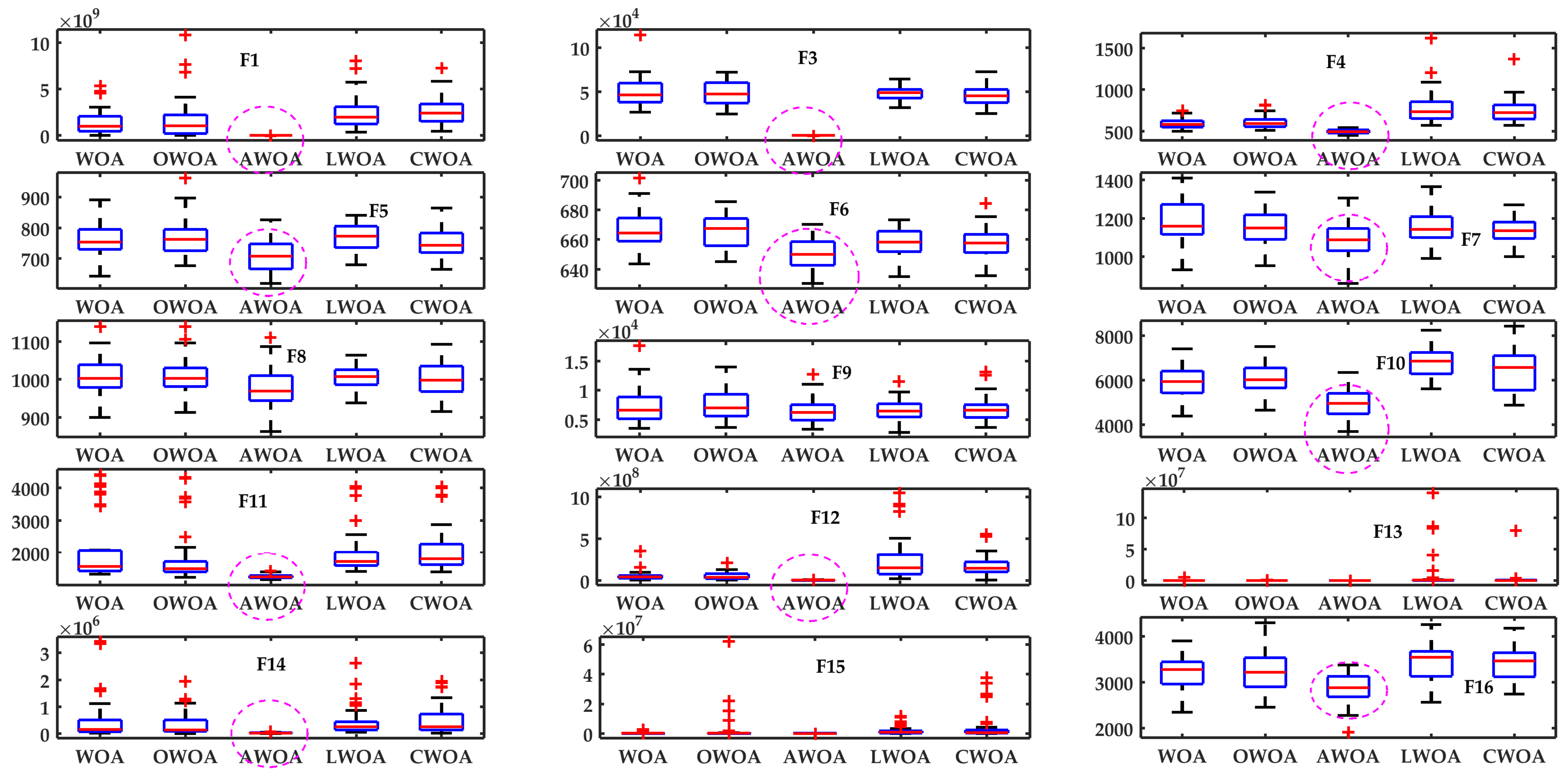
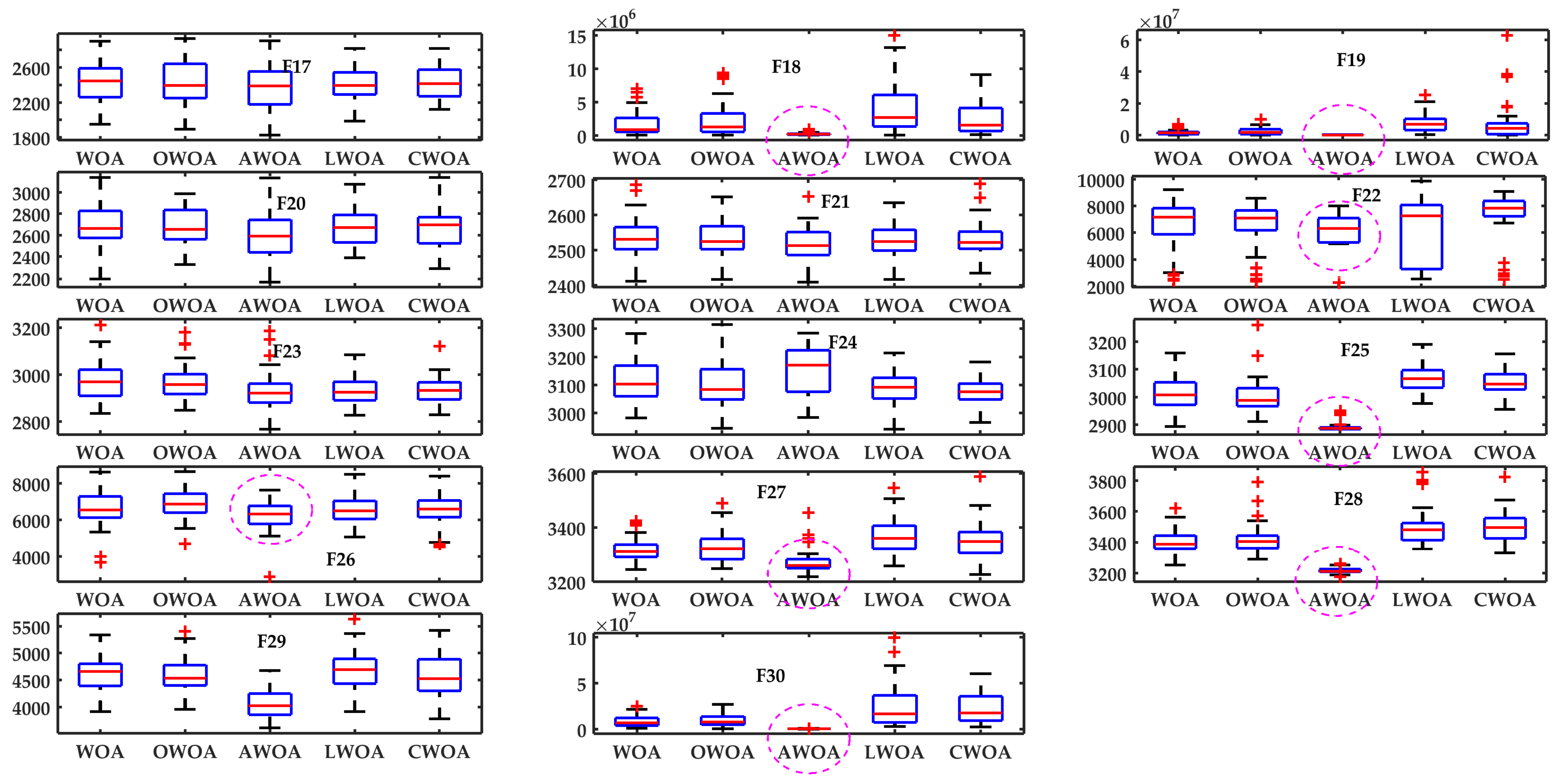
5.3.2. Boxplot Analysis

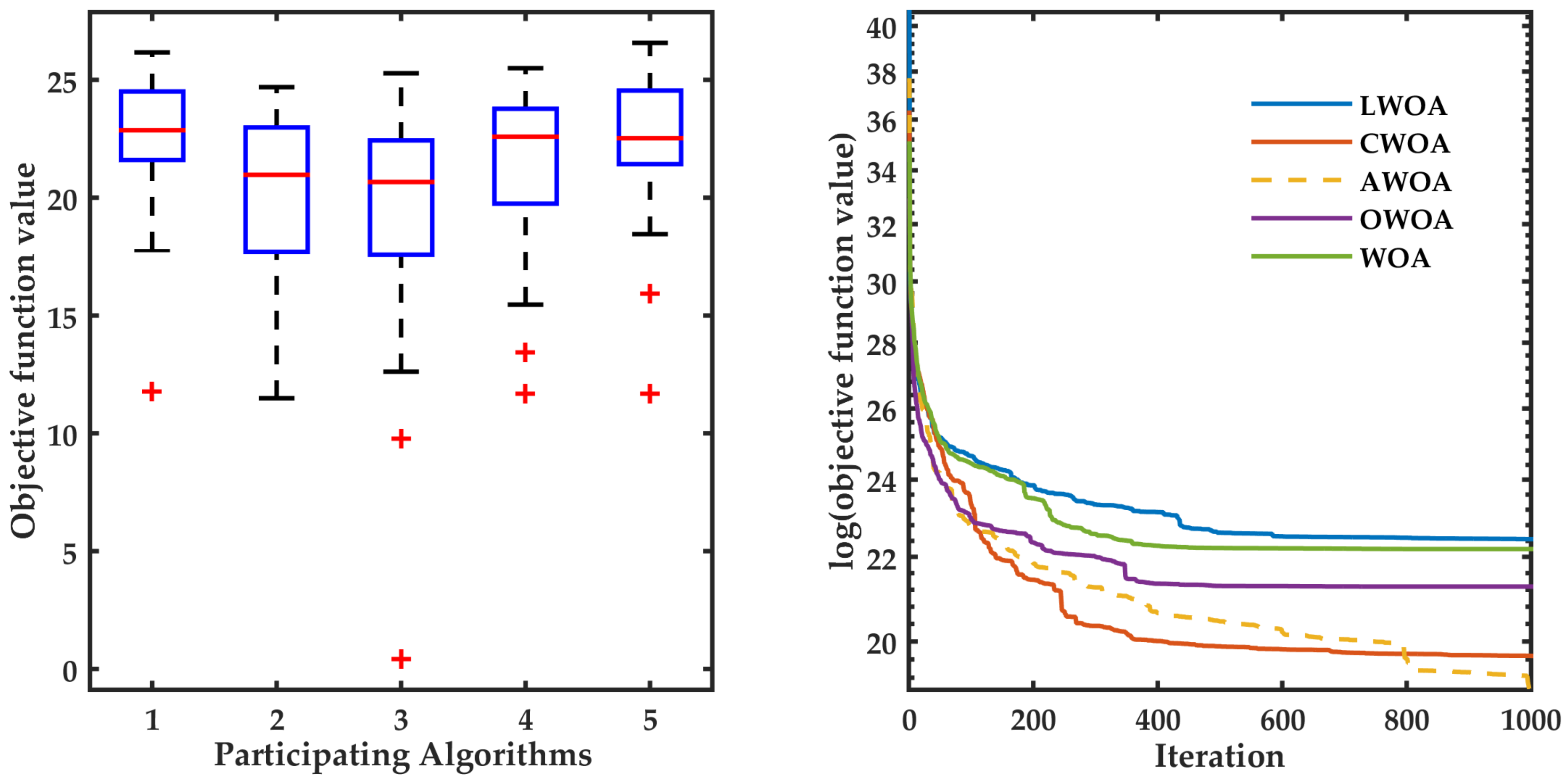
Boxplot analysis for 10D functions are performed for 20 independent runs of objective function values. This analysis is depicted in Figure 9 and Figure 10. From these boxplots, it is easily to state that the results obtained from the optimization process acquire an optimal Inter Quartile Range and low mean values. For showcasing the efficacy of the proposed AWOA, all the optimal entries of mean values are depicted with an oval shape in boxplots.

5.4. Results of the Analysis of 30D Problems

The results of the proposed AWOA, along with other variants of WOA, are depicted in terms of statistical attributes of independent 51 runs in Table 6. From the results, it is clearly evident that except for F24, the proposed AWOA provides optimal results as compared to other opponents. Mean values of objective functions and standard deviation of the objective functions obtained from independent runs are shown in bold face.

The results of the rank sum test are depicted in Table 8. It is always important to judge the statistical significance of the optimization run in terms of calculated p-values. For this reason, the proposed AWOA was compared with all opponents and the results in terms of p-values are depicted. Bold face entries show that there is a significance difference between optimization runs obtained in AWOA and other opponent, as the obtained p-values are less than 0.05. We observe that for the majority of the functions, calculated p-values are less than 0.05. 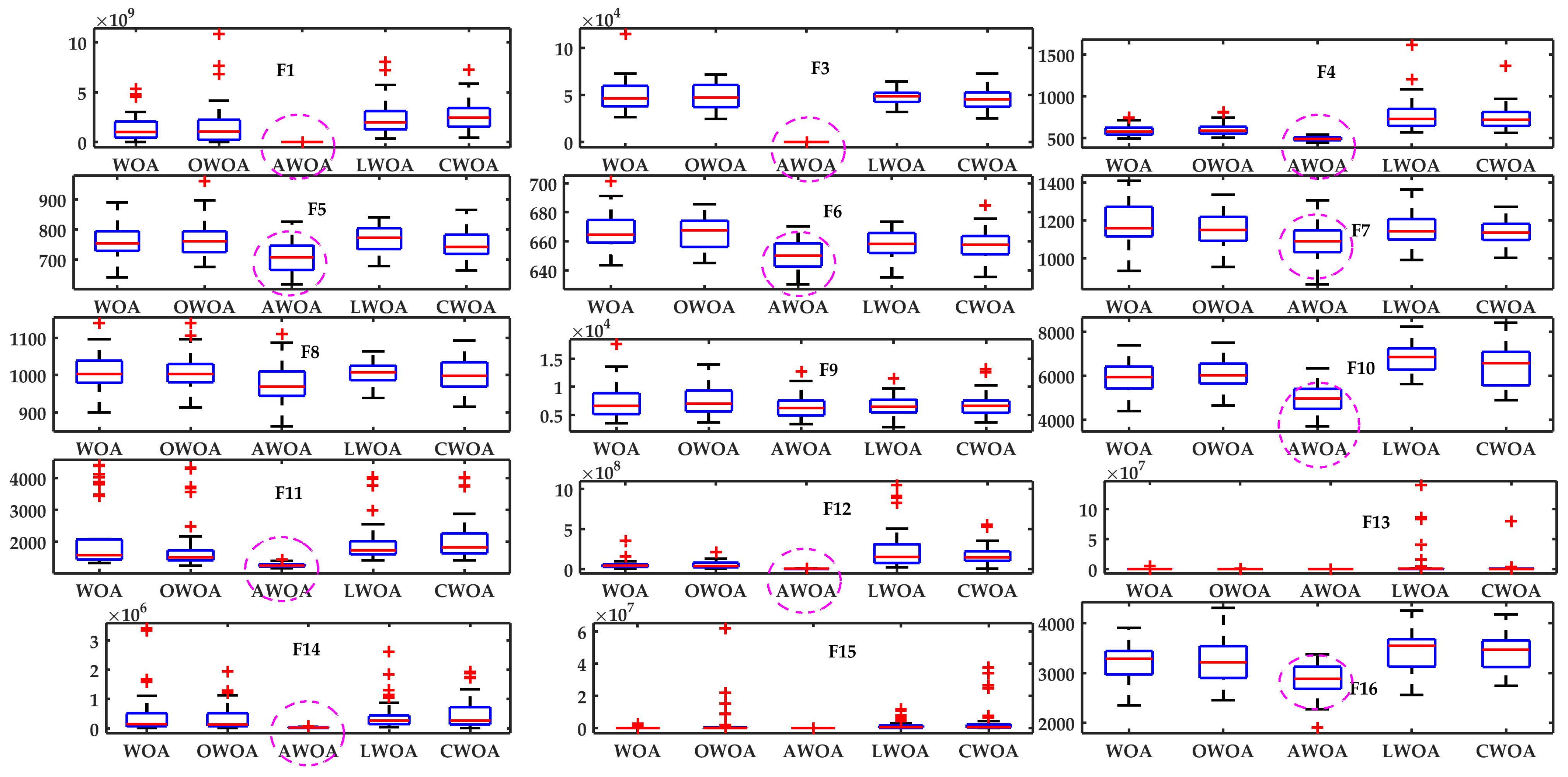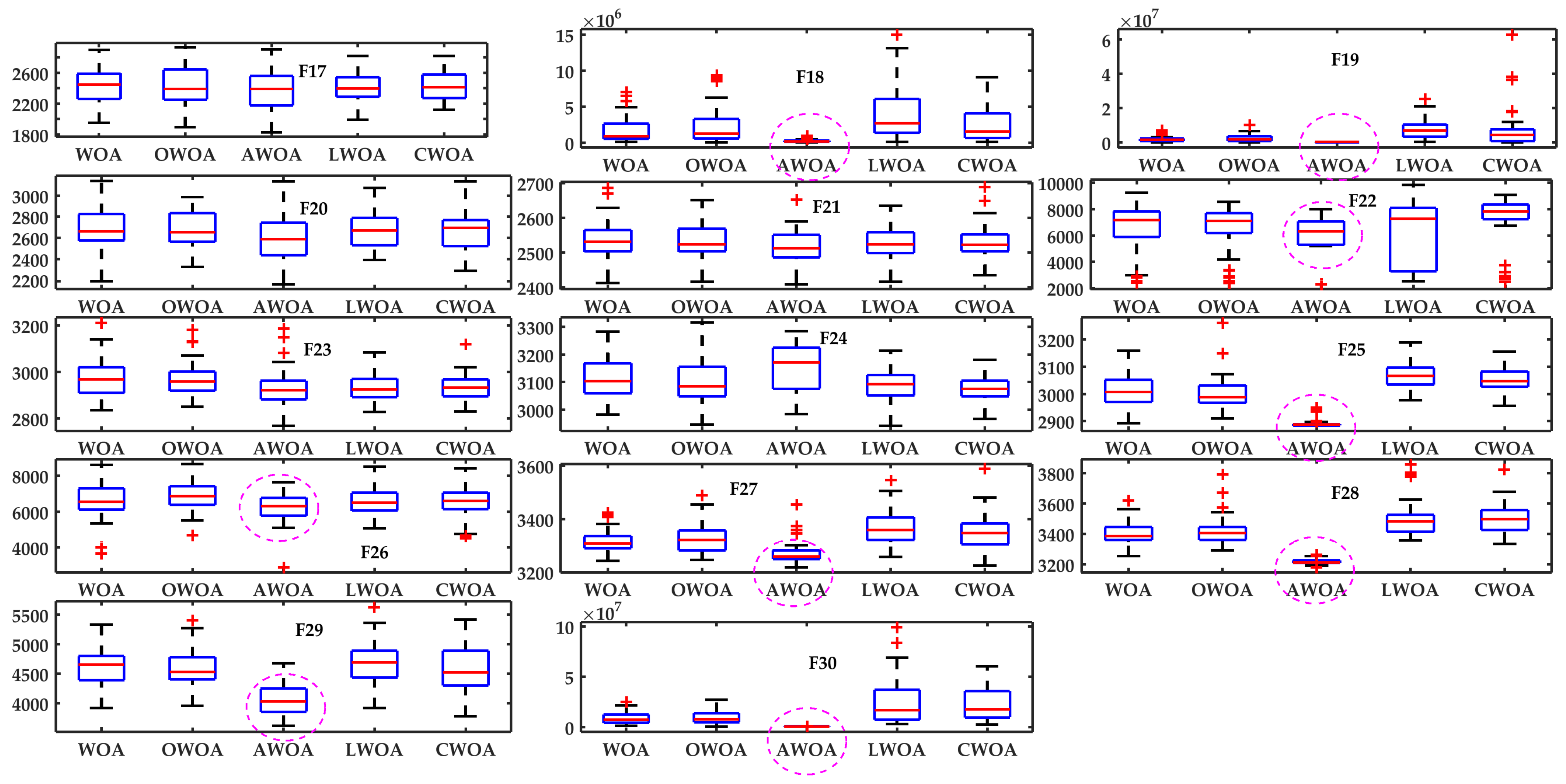Along with the optimal mean and standard deviation values, p-values indicated that the proposed AWOA outperforms. 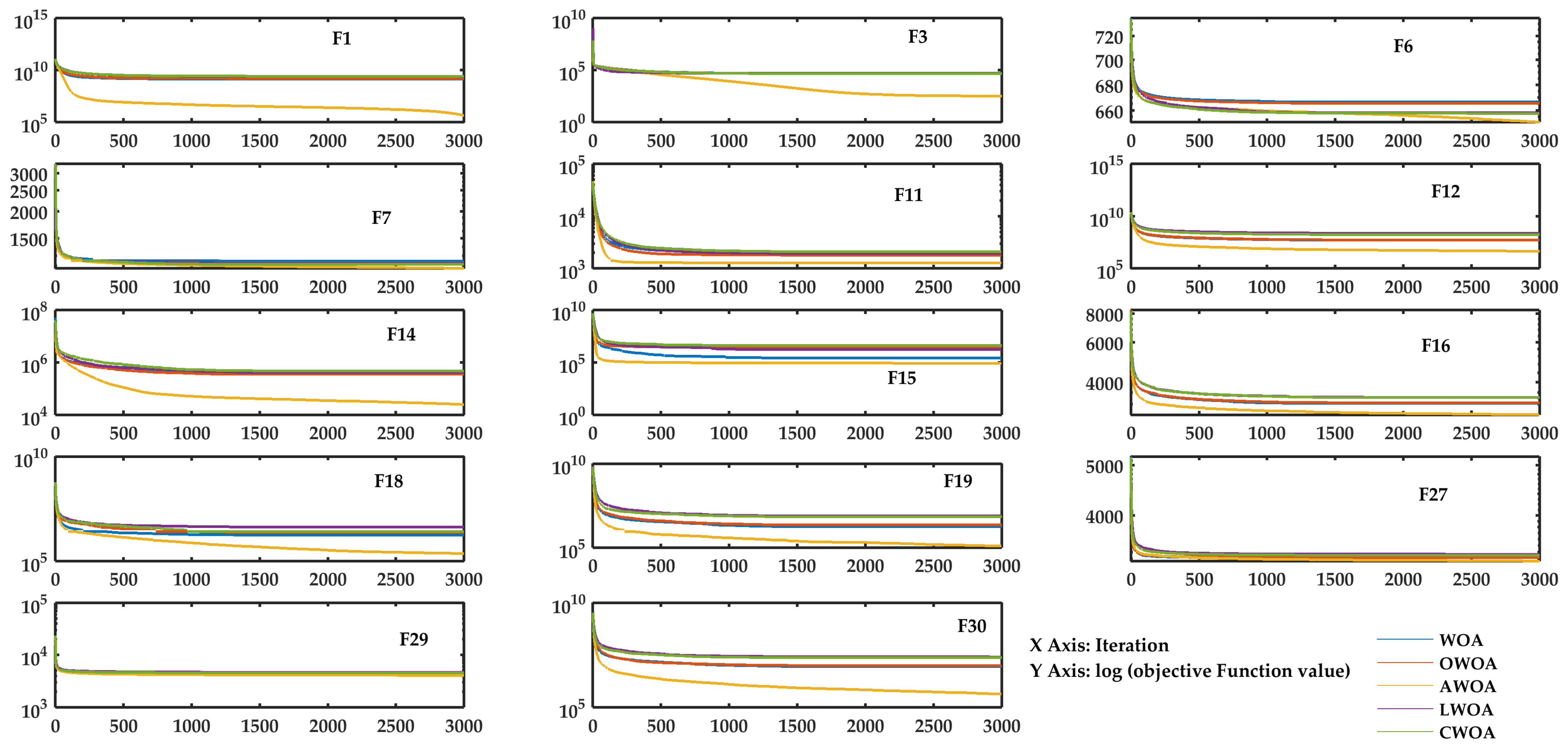In addition to these analyses, a boxplot analysis was performed of the proposed AWOA with other opponents, as depicted in Figure 11 and Figure 12. From these figures, it is easy to learn that the IQR and mean values are very competitive and optimal in almost all cases for 30-dimension problems. Inspecting the convergence curves for some of the functions, such as unimodal functions F1 and F3 and for some other multimodal and hybrid functions, as depicted in Figure 13.

5.5. Comparison with Other Algorithms

To validate the efficacy of the proposed variant, a fair comparison on CEC 2017 criteria is executed. The optimization results of the proposed variant along with some contemporary and classical optimizers are reported in

Table 9. Comparison of AWOA with other algorithms for 30D.

	Algorithm
Function	SCA	PSO	MFO	FPA	AWOA
F1	1.27 $\times {10}^{10}$	5.56 $\times {10}^9$	1.31 $\times {10}^{10}$	1.07 $\times {10}^8$	4.53 $\times {10}^5$
F3	3.67 $\times {10}^4$	1.33 $\times {10}^5$	9.48 $\times {10}^4$	1.10 $\times {10}^5$	3.24 $\times {10}^2$
F4	9.90 $\times {10}^2$	5.09 $\times {10}^2$	9.70 $\times {10}^2$	5.79 $\times {10}^2$	4.95 $\times {10}^2$
F5	2.75 $\times {10}^2$	3.04 $\times {10}^2$	2.20 $\times {10}^2$	8.06 $\times {10}^2$	7.13 $\times {10}^2$
F6	5.00 $\times {10}^1$	5.60 $\times {10}^1$	4.00 $\times {10}^1$	6.69 $\times {10}^2$	6.51 $\times {10}^2$
F7	4.30 $\times {10}^2$	4.30 $\times {10}^2$	4.60 $\times {10}^2$	1.33 $\times {10}^3$	1.09 $\times {10}^3$
F8	2.50 $\times {10}^2$	2.90 $\times {10}^2$	2.20 $\times {10}^2$	1.07 $\times {10}^3$	9.80 $\times {10}^2$
F9	4.74 $\times {10}^3$	5.70 $\times {10}^3$	6.57 $\times {10}^3$	1.31 $\times {10}^4$	6.48 $\times {10}^3$
F10	7.13 $\times {10}^3$	8.29 $\times {10}^3$	4.34 $\times {10}^3$	6.20 $\times {10}^3$	4.98 $\times {10}^3$
F11	9.70 $\times {10}^2$	2.54 $\times {10}^3$	5.30 $\times {10}^3$	1.54 $\times {10}^3$	1.27 $\times {10}^3$
F12	1.18 $\times {10}^9$	6.47 $\times {10}^8$	3.81 $\times {10}^8$	4.84 $\times {10}^7$	4.36 $\times {10}^6$
F13	3.96 $\times {10}^8$	1.93 $\times {10}^8$	9.52 $\times {10}^7$	2.61 $\times {10}^6$	1.46 $\times {10}^5$
F14	1.53 $\times {10}^5$	1.11 $\times {10}^6$	2.32 $\times {10}^5$	1.66 $\times {10}^5$	2.46 $\times {10}^4$
F15	1.62 $\times {10}^7$	3.91 $\times {10}^7$	5.21 $\times {10}^4$	4.22 $\times {10}^5$	7.96 $\times {10}^4$
F16	2.04 $\times {10}^3$	2.35 $\times {10}^3$	1.55 $\times {10}^3$	3.46 $\times {10}^3$	2.87 $\times {10}^3$
F17	7.00 $\times {10}^2$	9.60 $\times {10}^2$	8.80 $\times {10}^2$	2.71 $\times {10}^3$	2.37 $\times {10}^3$
F18	3.16 $\times {10}^6$	7.90 $\times {10}^6$	3.19 $\times {10}^6$	3.17 $\times {10}^6$	2.29 $\times {10}^5$
F19	2.37 $\times {10}^7$	5.17 $\times {10}^7$	2.42 $\times {10}^7$	2.30 $\times {10}^6$	1.22 $\times {10}^5$
F20	6.10 $\times {10}^2$	1.02 $\times {10}^3$	6.80 $\times {10}^2$	2.64 $\times {10}^3$	2.60 $\times {10}^3$
F21	4.60 $\times {10}^2$	5.00 $\times {10}^2$	4.10 $\times {10}^2$	2.57 $\times {10}^3$	2.51 $\times {10}^3$
F22	5.78 $\times {10}^3$	4.64 $\times {10}^3$	4.27 $\times {10}^3$	6.11 $\times {10}^3$	5.69 $\times {10}^3$
F23	6.90 $\times {10}^3$	7.80 $\times {10}^2$	5.30 $\times {10}^2$	3.00 $\times {10}^3$	2.93 $\times {10}^3$
F24	7.60 $\times {10}^2$	8.10 $\times {10}^2$	5.90 $\times {10}^2$	3.13 $\times {10}^3$	3.15 $\times {10}^3$
F25	7.10 $\times {10}^2$	7.10 $\times {10}^2$	8.30 $\times {10}^2$	2.97 $\times {10}^3$	2.89 $\times {10}^3$
F26	4.34 $\times {10}^3$	4.05 $\times {10}^3$	3.26 $\times {10}^3$	7.63 $\times {10}^3$	6.12 $\times {10}^3$
F27	7.00 $\times {10}^2$	6.60 $\times {10}^2$	5.60 $\times {10}^2$	3.34 $\times {10}^3$	3.27 $\times {10}^3$
F28	1.00 $\times {10}^3$	8.40 $\times {10}^2$	1.76 $\times {10}^3$	3.35 $\times {10}^3$	3.22 $\times {10}^3$
F29	1.73 $\times {10}^3$	2.02 $\times {10}^3$	1.25 $\times {10}^3$	4.64 $\times {10}^3$	4.06 $\times {10}^3$
F30	6.69 $\times {10}^7$	4.85 $\times {10}^7$	1.02 $\times {10}^6$	6.79 $\times {10}^6$	4.28 $\times {10}^5$

. The competitive algorithms are Moth flame optimization (MFO) [15], Sine cosine algorithm [53], PSO [54] and Flower pollination Algorithm [55]. It can be easily observed that the results of our proposed variant are competitive for almost all the functions.

6. Applications of AWOA in Engineering Test Problems

6.1. Model Order Reduction

In control system engineering, most of the linear time invariant systems are of a higher order, and thus, difficult to analyze. This problem has been solved using the reduced model order technique, which is easy to use and less complex in comparison to earlier control paradigm techniques. Nature-inspired optimization algorithms have proved to be an efficient tool in this field, as they help to minimize the integral square of lower-order systems. This approach was first introduced in [56] followed by [39,57,58] and many more. These works advocate the efficacy of optimization algorithm in solving the reduced model order technique, as these reduce the complexity, computation time and cost of the reducing process. For testing the applicability of AWOA on some real-world problems, we have considered the Model Order Reduction problem in this section. In MOR, large complex systems with known transfer functions are converted with the help of an optimization application to the reduced order system. The following are the steps of the conversion:

• Consider a large complex system with a higher order and obtain the step response of the system. Stack the response in the form of a numerical array.
• Construct a second-order system with the help of some unknown variables that are depicted in the following equation. Furthermore, obtain the step response of the system and stack those numbers in a numerical array.
• Construct a transfer function that minimizes the error function, preferably the Integral Square Error (ISE) criterion.

6.1.1. Problem Formulation

In this technique, a transfer function given by $X\left(t\right):u\to v$ of a higher order is reduced, in function $X\left(t\right):u\to \tilde{v}$ of a lower order, without affecting the input $u\left(x\right)$; the output is $\tilde{v}\left(x\right)\approx v\left(x\right)$. The integral error defined by the following equation is minimized in the process using the optimization algorithm:

$$\mathrm{IE}=\underset{0}{\overset{\infty }{\int }}{\left[v\left(x\right)-\tilde{v}\left(x\right)\right]}^{2}dx$$

(17)

where $X\left(t\right)$ is a transfer function of any Single Input and Single Output system defined by:

$$X\left(s\right)=\frac{a_0+a_{1}t+a_2{t}^2+\dots +a_m{t}^m}{b_0+b_{1}t+b_2{t}^2+\dots +b_n{t}^n}$$

(18)

For a reduced order system, $X{\left(s\right)}^{\prime }$ can be given by:

$$X{\left(t\right)}^{\prime }=\frac{a_0^{\prime }+a_1^{\prime }t+a_2^{\prime }{t}^2+\dots +a_{m_r}^{\prime }{t}^{m_r}}{b_0^{\prime }+b_1^{\prime }t+b_2^{\prime }{t}^2+\dots +b_{n_r}^{\prime }{t}^{n_r}}$$

(19)

where $(n_r\ge m_r,m_r,n_r\in I)$. In this study, we calculate the value of coefficients of the numerator and denominator of a reduced order system defined in Equation (21) while minimizing the error. To establish the efficiency of our proposed variant, we have reported two numerical examples.

6.1.2. Numerical Examples and Discussions

• Function 1

  $$X\left(s\right)=\frac{(s^3+7s^2+24s+24)}{(s^4+10s^3+35s^2+50s+24)}$$

  (20)
• Function 2

  $$X\left(s\right)=\frac{(s+4)}{(s^4+19s^3+113s^2+245s+150)}$$

  (21)

The results of the optimization process by depicting the values of time domain specifications, namely rise time and settling time for both functions, are exhibited in

Table 10. Simulated models for different WOA variants and time domain specifications.

Function	Function 1		Function 2
Parameters	Rise Time	Settling Time	Rise Time	Settling Time
Original	2.1398	4.8603	2.2985	4.9724
AWOA	2.1471	4.8388	2.2649	4.3923
WOA	2.0838	4.6762	3.1631	6.6672
OWOA	2.4744	5.4009	3.1783	6.689
LWOA	2.1002	4.7188	2.4078	5.1828
CWOA	2.45	4.965	3.1755	6.68

. Furthermore, the convergence proofs of the algorithm on both functions are depicted in Figure 14 and Figure 15. Errors in the time domain specifications as compared to the original system are depicted in

Table 11. Error analysis of MOR results on both functions.

Parameter	% Error Function 1		% Error Function 2
Time	Rise Time	Settling Time	Rise Time	Settling Time
AWOA	0.341	0.442	1.462	11.666
WOA	2.617	3.788	37.616	34.084
OWOA	15.637	11.123	38.277	34.523
LWOA	1.851	2.911	4.755	4.231
CWOA	14.497	2.154	38.155	34.342

.

From these analyses, it is quite evident that MOR performed by AWOA leads to a configuration of the system that follows the time domain specifications of the original system quite closely. In addition to that, the error in objective function values are also optimal in the case of AWOA.

6.2. Frequency-Modulated Sound Wave Parameter Estimation Problem

This problem has been taken in many approaches to benchmark the applicability of different optimizers. This problem was included in the 2011 Congress on Evolutionary computation competition for testing different evolutionary optimization algorithms on real problems [59]. This problem is a six-dimensional problem, where the parameters of a sound wave are estimated in such a manner that it should be matched with the target wave.

The mathematical representation of this problem can be given as:

$$K=\left({\alpha }_1,{\delta }_1,{\alpha }_2,{\delta }_2,{\alpha }_3,{\delta }_3\right)$$

(22)

The equations of the predicted sound wave and target sound wave are as follows:

$$J\left(t\right)={\alpha }_1.sin\left({\delta }_1.t.\theta +{\alpha }_2.sin\left({\delta }_2.t.\theta +{\alpha }_3.sin\left({\delta }_3.t.\theta \right)\right)\right)$$

(23)

$$J_0\left(t\right)=\left(1.0\right).sin\left(\left(5.0\right).t.\theta -\left(1.5\right).sin\left(\left(4.8\right).t.\theta +\left(2.0\right).sin\left(\left(4.9\right)t.\theta \right)\right)\right)$$

(24)

$$Min f(\overrightarrow{K})={\displaystyle \sum _{t=0}^{100}}{(J\left(t\right)-J_0\left(t\right))}^2$$

(25)

The results of this design problem are shown in terms of different analyses that include the boxplot and convergence property, which are obtained from 20 independent runs. The Figure 16 shows this analysis. A comparison of the performance on the basis of error in the objective function values is depicted in Figure 17. Here, boxplot axis entry 1, 2, 3, 4 and 5 show LWOA, CWOA, proposed AWOA, OWOA and WOA, respectively.

6.3. PID Control of DC Motors

In today’s machinery era, DC motors are used in various fields such as the textile industry, rolling mills, electric vehicles and robotics. Among the various controllers available for DC motors, the Proportional Integral Derivative (PID) is the most widely used and proved its efficiency as an accurate result provider without disturbing the steady state error and overshoot phenomena [60]. With this controller, we also needed an efficient tuning method to control the speed and other parameters of DC motors. In recent years, some researchers have explored the meta-heuristic algorithm in tuning of different types of PID controllers. In [61], the authors presented a comparative study between simulated annealing, particle swarm optimization and genetic algorithm. Stochastic fractal search has been applied to the DC motor problem in [62]. The sine cosine algorithm is also used in the determination of optimal parameters of the PID controller of DC motors in [20]. In [63], the authors proposed the chaotic atom search optimization for optimal tuning of the PID controller of DC motors with a fractional order. A hybridized version of foraging optimization and simulated annealing to solve the same problem was reported in [64].

6.3.1. Mathematical Model of DC Motors

The DC motor problem used here is a specific type of DC motor which controlled its speed through input voltage or change in current. In DC motors, the applied voltage $f_b\left(t\right)$ is directly proportional to the angular speed $\beta \left(t\right)=\frac{d\alpha \left(t\right)}{dt}$, while the flux is constant, i.e.:

$$f_b\left(t\right)=H_b\frac{d\alpha \left(t\right)}{dt}=H_b\beta \left(t\right)$$

(26)

The initial voltage of armature $f_a\left(t\right)$ satisfies the following differential equation:

$$f_b\left(t\right)=P_a\frac{d{r}_a\left(t\right)}{dt}+K_a{r}_a\left(t\right)+f_a\left(t\right)$$

(27)

The motor torque (due to various friction) developed in the process (neglecting the disturbance torque) is given by:

$$\tau \left(t\right)=L\frac{d\beta \left(t\right)}{dt}+T\beta \left(t\right)=H_m{r}_a\left(t\right)$$

(28)

Taking the Laplace transform of these equations and assuming all the initial condition to zero, we get:

$$F_b\left(s\right)=H_{b}X\left(s\right)$$

(29)

$$F_a\left(s\right)=(P_{a}s+K_a)R_a\left(s\right)+F_b\left(s\right)$$

(30)

$$\Omega \left(s\right)=(Ls+T)X\left(s\right)=H_m{R}_a\left(s\right)$$

(31)

On simplifying these equations, open loop transfer function of DC motor can be given as:

$$\frac{X\left(s\right)}{F_a\left(s\right)}=\frac{H_m}{(P_{a}s+K_a)(Ls+T)+H_b{H}_m}$$

(32)

6.3.2. Results and Discussion

All the parameters and constant values considered in this experiment are given in

Table 12. Various parameters of DC motors.

Motor Parameter	Symbol	Value
Resistance	$K_a$	0.4 $\omega$
Inductance	$P_a$	2.7 H
Initial torque of motor	L	0.0004 kg m2
constant of friction in motor	T	0.0022 Nm s/rad2
Motor torque	$H_m$	0.015 Nm/A
Emf constant	$H_b$	0.05 V s/rad

. The simulation results for tuning the PID controller for plant DC motors are depicted in

Table 13. Comparison of AWOA with other algorithms for the DC motor controller design problem.

Algorithm	DC Motor Closed Loop Transfer Function	Settling Time	Rise Time
OWOA	$\frac{0.03684s^2+0.2999s+0.1358}{0.00108s^3+0.04438s^2+0.3095s+0.1358}$	0.0994	0.0603
WOA	$\frac{0.03623s^2+0.3s+0.106}{0.00108s^3+0.04377s^2+0.3095s+0.106}$	0.0997	0.0609
CWOA	$\frac{0.03703s^2+0.3s+0.1447}{0.00108s^3+0.04457s^2+0.3095s+0.1447}$	0.0993	0.0602
LWOA	$\frac{0.03664s^2+0.3s+0.1255}{0.00108s^3+0.04418s^2+0.3095s+0.1255}$	0.0995	0.0605
AWOA	$\frac{0.03703s^2+0.3s+0.1447}{0.00108s^3+0.04457s^2+0.3095s+0.1447}$	0.0991	0.0598

. First column entries show the plant and controller combined realization as a closed system and the other two entries show specification of time domain simulation conducted when the system is subjected to step input.

After a careful observation, it is concluded that the closed loop system realized with the proposed AWOA possesses optimal settling and rise time that itself depicts a fast transient response of the system. Although the comparative analysis of other algorithms also depicts very competitive values of these times, the response and convergence process of AWOA are swift as compared to other opponents. The boxplot analysis and convergence property analysis are shown in Figure 18. The boxplot shows the comparison of the optimization results when the optimization is run 20 independent times. The X axis shows the AWOA, CWOA, LWOA, OWOA and WOA algorithms. The optimal entries of settling time and rise time are in bold face to showcase the efficacy of the AWOA. The step response of these controllers has been shown in Figure 19.

7. Conclusions

This paper is a proposal of a new variant of WOA. The singing behavior of whales is mimicked with the help of opposition-based learning in the initialization phase and Cauchy mutation in the position update phase. The following are the major conclusions drawn from this study:

• The proposed AWOA was validated on two benchmark suits (conventional and CEC 2017 functions). These benchmark suits comprise mathematical functions of distinct nature (unimodal, multimodal, hybrid and composite). We have observed that for the majority of the functions, AWOA shows promising results. It is also observed that the performance of AWOA is competitive with other algorithms.
• The statistical significance of the obtained results is verified with the help of a boxplot analysis and Wilcoxon rank sum test. It is observed that boxplots are narrow for the proposed AWOA and the p-values are less than 0.05. These results show that the proposed variant exhibits better exploration and exploitation capabilities, and with these results, one can easily see the positive implications of the proposed modifications.
• The proposed variant is also tested for challenging engineering design problems. The first problem is the model order reduction of a complex control system into subsequent reduced order realizations. For this problem, AWOA shows promising results as compared to WOA. As a second problem, the frequency-modulated sound wave parameter estimation problem was addressed. The performance of the proposed AWOA is competitive with contemporary variants of WOA. In addition to that, the application of AWOA was reported for tuning the PID controller of the DC motor control system. All these applications indicate that the modifications suggested for AWOA are quite meaningful and help the algorithm find global optima in an effective way.

The proposed AWOA can be applied to various other engineering design problem, such as network reconfiguration, solar cell parameter extraction and regulator design. These problems will be the focus of future research.

References

1. Yang, X.S. Nature-Inspired Metaheuristic Algorithms; Luniver Press: Beckington, UK, 2010. [Google Scholar]
2. Glover, F. Future paths for integer programming and links to artificial intelligence. Comput. Oper. Res. 1986, 13, 533–549. [Google Scholar] [CrossRef]
3. Holland, J.H. Genetic algorithms. Sci. Am. 1992, 267, 66–73. [Google Scholar] [CrossRef]
4. Rechenberg, I. Evolution strategy: Nature’s way of optimization. In Optimization: Methods and Applications, Possibilities and Limitations; Springer: Berlin/Heidelberg, Germany, 1989; pp. 106–126. [Google Scholar]
5. Dorigo, M.; Di Caro, G. Ant colony optimization: A new meta-heuristic. In Proceedings of the 1999 Congress on Evolutionary Computation-CEC99 (Cat. No. 99TH8406), IEEE, Washington, DC, USA, 6–9 July 1999; Volume 2, pp. 1470–1477. [Google Scholar]
6. Basturk, B. An artificial bee colony (ABC) algorithm for numeric function optimization. In Proceedings of the IEEE Swarm Intelligence Symposium, Indianapolis, IN, USA, 12–14 May 2006. [Google Scholar]
7. Yang, X.S. A new metaheuristic bat-inspired algorithm. In Nature Inspired Cooperative Strategies for Optimization (NICSO 2010); Springer: Berlin/Heidelberg, Germany, 2010; pp. 65–74. [Google Scholar]
8. Yang, X.S.; Deb, S. Cuckoo search via Lévy flights. In Proceedings of the 2009 World Congress on Nature & Biologically Inspired Computing (NaBIC), Coimbatore, India, 9–11 December 2009; pp. 210–214. [Google Scholar]
9. Gandomi, A.H.; Alavi, A.H. Krill herd: A new bio-inspired optimization algorithm. Commun. Nonlinear Sci. Numer. Simul. 2012, 17, 4831–4845. [Google Scholar] [CrossRef]
10. Yang, X.S. Firefly algorithm, stochastic test functions and design optimisation. Int. J. Bio-Inspir. Comput. 2010, 2, 78–84. [Google Scholar] [CrossRef]
11. Mirjalili, S.; Mirjalili, S.M.; Lewis, A. Grey wolf optimizer. Adv. Eng. Softw. 2014, 69, 46–61. [Google Scholar] [CrossRef] [Green Version]
12. Das, S.; Biswas, A.; Dasgupta, S.; Abraham, A. Bacterial foraging optimization algorithm: Theoretical foundations, analysis, and applications. In Foundations of Computational Intelligence; Springer: Berlin/Heidelberg, Germany, 2009; Volume 3, pp. 23–55. [Google Scholar]
13. James, J.; Li, V.O. A social spider algorithm for global optimization. Appl. Soft Comput. 2015, 30, 614–627. [Google Scholar]
14. Chu, S.C.; Tsai, P.W.; Pan, J.S. Cat swarm optimization. In Pacific Rim International Conference on Artificial Intelligence; Springer: Berlin/Heidelberg, Germany, 2006; pp. 854–858. [Google Scholar]
15. Mirjalili, S. Moth-flame optimization algorithm: A novel nature-inspired heuristic paradigm. Knowl.-Based Syst. 2015, 89, 228–249. [Google Scholar] [CrossRef]
16. Mirjalili, S. The ant lion optimizer. Adv. Eng. Softw. 2015, 83, 80–98. [Google Scholar] [CrossRef]
17. Askarzadeh, A. A novel metaheuristic method for solving constrained engineering optimization problems: Crow search algorithm. Comput. Struct. 2016, 169, 1–12. [Google Scholar] [CrossRef]
18. Saremi, S.; Mirjalili, S.; Lewis, A. Grasshopper optimisation algorithm: Theory and application. Adv. Eng. Softw. 2017, 105, 30–47. [Google Scholar] [CrossRef] [Green Version]
19. Mohamed, A.W.; Hadi, A.A.; Mohamed, A.K. Gaining-sharing knowledge based algorithm for solving optimization problems: A novel nature-inspired algorithm. Int. J. Mach. Learn. Cybern. 2020, 11, 1501–1529. [Google Scholar] [CrossRef]
20. Agarwal, J.; Parmar, G.; Gupta, R. Application of sine cosine algorithm in optimal control of DC motor and robustness analysis. Wulfenia J. 2017, 24, 77–95. [Google Scholar]
21. Agrawal, P.; Ganesh, T.; Mohamed, A.W. Chaotic gaining sharing knowledge-based optimization algorithm: An improved metaheuristic algorithm for feature selection. Soft Comput. 2021, 25, 9505–9528. [Google Scholar] [CrossRef]
22. Agrawal, P.; Ganesh, T.; Mohamed, A.W. A novel binary gaining–sharing knowledge-based optimization algorithm for feature selection. Neural Comput. Appl. 2021, 33, 5989–6008. [Google Scholar] [CrossRef]
23. Agrawal, P.; Ganesh, T.; Oliva, D.; Mohamed, A.W. S-shaped and v-shaped gaining-sharing knowledge-based algorithm for feature selection. Appl. Intell. 2022, 52, 81–112. [Google Scholar] [CrossRef]
24. Erol, O.K.; Eksin, I. A new optimization method: Big bang–big crunch. Adv. Eng. Softw. 2006, 37, 106–111. [Google Scholar] [CrossRef]
25. Hatamlou, A. Black hole: A new heuristic optimization approach for data clustering. Inf. Sci. 2013, 222, 175–184. [Google Scholar] [CrossRef]
26. Rashedi, E.; Nezamabadi-Pour, H.; Saryazdi, S. GSA: A gravitational search algorithm. Inf. Sci. 2009, 179, 2232–2248. [Google Scholar] [CrossRef]
27. Formato, R.A. Central force optimization. Prog. Electromagn. Res. 2007, 77, 425–491. [Google Scholar] [CrossRef] [Green Version]
28. Kaveh, A.; Talatahari, S. A novel heuristic optimization method: Charged system search. Acta Mech. 2010, 213, 267–289. [Google Scholar] [CrossRef]
29. Azadeh, A.; Asadzadeh, S.M.; Jalali, R.; Hemmati, S. A greedy randomised adaptive search procedure–genetic algorithm for electricity consumption estimation and optimisation in agriculture sector with random variation. Int. J. Ind. Syst. Eng. 2014, 17, 285–301. [Google Scholar] [CrossRef]
30. Blum, C.; Pinacho, P.; López-Ibáñez, M.; Lozano, J.A. Construct, merge, solve & adapt a new general algorithm for combinatorial optimization. Comput. Oper. Res. 2016, 68, 75–88. [Google Scholar]
31. Thiruvady, D.; Blum, C.; Ernst, A.T. Solution merging in matheuristics for resource constrained job scheduling. Algorithms 2020, 13, 256. [Google Scholar] [CrossRef]
32. Wolpert, D.H.; Macready, W.G. No Free Lunch Theorems for Search; Technical Report; Technical Report SFI-TR-95-02-010; Santa Fe Institute: Santa Fe, NM, USA, 1995. [Google Scholar]
33. Lones, M.A. Mitigating metaphors: A comprehensible guide to recent nature-inspired algorithms. SN Comput. Sci. 2020, 1, 1–12. [Google Scholar] [CrossRef] [Green Version]
34. Mirjalili, S.; Lewis, A. The whale optimization algorithm. Adv. Eng. Softw. 2016, 95, 51–67. [Google Scholar] [CrossRef]
35. Kaveh, A.; Ghazaan, M.I. Enhanced whale optimization algorithm for sizing optimization of skeletal structures. Mech. Based Des. Struct. Mach. 2017, 45, 345–362. [Google Scholar] [CrossRef]
36. Touma, H.J. Study of the economic dispatch problem on IEEE 30-bus system using whale optimization algorithm. Int. J. Eng. Technol. Sci. (IJETS) 2016, 5, 11–18. [Google Scholar] [CrossRef]
37. Ladumor, D.P.; Trivedi, I.N.; Jangir, P.; Kumar, A. A whale optimization algorithm approach for unit commitment problem solution. In Proceedings of the National Conference on Advancements in Electrical and Power Electronics Engineering (AEPEE-2016), Morbi, India, 28–29 June 2016; pp. 4–17. [Google Scholar]
38. Cui, D. Application of whale optimization algorithm in reservoir optimal operation. Adv. Sci. Technol. Water Resour. 2017, 37, 72–79. [Google Scholar]
39. Saxena, A. A comprehensive study of chaos embedded bridging mechanisms and crossover operators for grasshopper optimisation algorithm. Expert Syst. Appl. 2019, 132, 166–188. [Google Scholar] [CrossRef]
40. Ibrahim, R.A.; Elaziz, M.A.; Lu, S. Chaotic opposition-based grey-wolf optimization algorithm based on differential evolution and disruption operator for global optimization. Expert Syst. Appl. 2018, 108, 1–27. [Google Scholar] [CrossRef]
41. Elaziz, M.A.; Oliva, D. Parameter estimation of solar cells diode models by an improved opposition-based whale optimization algorithm. Energy Convers. Manag. 2018, 171, 1843–1859. [Google Scholar] [CrossRef]
42. Xu, Q.; Wang, L.; Wang, N.; Hei, X.; Zhao, L. A review of opposition-based learning from 2005 to 2012. Eng. Appl. Artif. Intell. 2014, 29, 1–12. [Google Scholar] [CrossRef]
43. Mahdavi, S.; Rahnamayan, S.; Deb, K. Opposition based learning: A literature review. Swarm Evol. Comput. 2018, 39, 1–23. [Google Scholar] [CrossRef]
44. Gupta, S.; Deep, K. Cauchy Grey Wolf Optimiser for continuous optimisation problems. J. Exp. Theor. Artif. Intell. 2018, 30, 1051–1075. [Google Scholar] [CrossRef]
45. Wang, G.G.; Zhao, X.; Deb, S. A novel monarch butterfly optimization with greedy strategy and self-adaptive. In Proceedings of the Soft Computing and Machine Intelligence (ISCMI), 2015 Second International Conference on IEEE, Hong Kong, China, 23–24 November 2015; pp. 45–50. [Google Scholar]
46. Digalakis, J.G.; Margaritis, K.G. On benchmarking functions for genetic algorithms. Int. J. Comput. Math. 2001, 77, 481–506. [Google Scholar] [CrossRef]
47. Molga, M.; Smutnicki, C. Test functions for optimization needs. Test Funct. Optim. Needs 2005, 101, 48. [Google Scholar]
48. Yang, X.S. Test problems in optimization. arXiv 2010, arXiv:1008.0549. [Google Scholar]
49. Awad, N.; Ali, M.; Liang, J.; Qu, B.; Suganthan, P. Problem Definitions and Evaluation Criteria for the CEC 2017 Special Session and Competition on Single Objective Bound Constrained Real-Parameter Numerical Optimization; Technical Report; Nanyang Technological University Singapore: Singapore, 2016. [Google Scholar]
50. Ling, Y.; Zhou, Y.; Luo, Q. Lévy flight trajectory-based whale optimization algorithm for global optimization. IEEE Access 2017, 5, 6168–6186. [Google Scholar] [CrossRef]
51. Oliva, D.; Abd El Aziz, M.; Hassanien, A.E. Parameter estimation of photovoltaic cells using an improved chaotic whale optimization algorithm. Appl. Energy 2017, 200, 141–154. [Google Scholar] [CrossRef]
52. Wilcoxon, F. Individual comparisons by ranking methods. Biom. Bull. 1945, 1, 80–83. [Google Scholar] [CrossRef]
53. Mirjalili, S. SCA: A sine cosine algorithm for solving optimization problems. Knowl.-Based Syst. 2016, 96, 120–133. [Google Scholar] [CrossRef]
54. Kennedy, J.; Eberhart, R. Particle swarm optimization. In Proceedings of the IEEE International Conference on Neural Networks IV, Perth, WA, Australia, 27 November–1 December 1995; Volume 1000. [Google Scholar]
55. Yang, X.S. Flower pollination algorithm for global optimization. In International Conference on Unconventional Computing and Natural Computation; Springer: Berlin/Heidelberg, Germany, 2012; pp. 240–249. [Google Scholar]
56. Biradar, S.; Hote, Y.V.; Saxena, S. Reduced-order modeling of linear time invariant systems using big bang big crunch optimization and time moment matching method. Appl. Math. Model. 2016, 40, 7225–7244. [Google Scholar] [CrossRef]
57. Dinkar, S.K.; Deep, K. Accelerated opposition-based antlion optimizer with application to order reduction of linear time-invariant systems. Arab. J. Sci. Eng. 2019, 44, 2213–2241. [Google Scholar] [CrossRef]
58. Shekhawat, S.; Saxena, A. Development and applications of an intelligent crow search algorithm based on opposition based learning. ISA Trans. 2020, 99, 210–230. [Google Scholar] [CrossRef]
59. Das, S.; Suganthan, P.N. Problem Definitions and Evaluation Criteria for CEC 2011 Competition on Testing Evolutionary Algorithms on Real World Optimization Problems; Jadavpur University: Kolkata, India; Nanyang Technological University: Singapore, 2010. [Google Scholar]
60. Shah, P.; Agashe, S. Review of fractional PID controller. Mechatronics 2016, 38, 29–41. [Google Scholar] [CrossRef]
61. Hsu, D.Z.; Chen, Y.W.; Chu, P.Y.; Periasamy, S.; Liu, M.Y. Protective effect of 3, 4-methylenedioxyphenol (sesamol) on stress-related mucosal disease in rats. BioMed Res. Int. 2013, 2013, 481827. [Google Scholar] [CrossRef]
62. Bhatt, R.; Parmar, G.; Gupta, R.; Sikander, A. Application of stochastic fractal search in approximation and control of LTI systems. Microsyst. Technol. 2019, 25, 105–114. [Google Scholar] [CrossRef]
63. Hekimoğlu, B. Optimal tuning of fractional order PID controller for DC motor speed control via chaotic atom search optimization algorithm. IEEE Access 2019, 7, 38100–38114. [Google Scholar] [CrossRef]
64. Ekinci, S.; Izci, D.; Hekimoğlu, B. Optimal FOPID Speed Control of DC Motor via Opposition-Based Hybrid Manta Ray Foraging Optimization and Simulated Annealing Algorithm. Arab. J. Sci. Eng. 2021, 46, 1395–1409. [Google Scholar] [CrossRef]
Figure 1. Development timeline of some of the leading bio-inspired algorithms.
Mathematics 10 02076 g001
Figure 2. Solving the one-dimensional problem by recursive halving the search interval.
Mathematics 10 02076 g002
Figure 3. Whale position update inspired from Cauchy Distribution.
Mathematics 10 02076 g003
Figure 4. Benchmark Suite 1.
Mathematics 10 02076 g004
Figure 5. Convergence property analysis of unimodal functions.
Mathematics 10 02076 g005
Figure 6. Convergence property analysis of multimodal functions.
Mathematics 10 02076 g006
Figure 7. Boxplot analysis of Benchmark Suite 1.
Mathematics 10 02076 g007
Figure 8. Boxplot analysis of the remaining functions of Benchmark Suite 1.
Mathematics 10 02076 g008
Figure 9. Boxplot analysis of the 10D functions of Benchmark Suite 2.
Mathematics 10 02076 g009
Figure 10. Boxplot analysis of the remaining 10D functions of Benchmark Suite 2.
Mathematics 10 02076 g010
Figure 11. Boxplot analysis of the 30D functions of Benchmark Suite 2.
Mathematics 10 02076 g011
Figure 12. Boxplot analysis of the remaining 30D functions of Benchmark Suite 2.
Mathematics 10 02076 g012
Figure 13. Convergence property analysis of some 30D functions of Benchmark Suite 2.
Mathematics 10 02076 g013
Figure 14. Results of MOR for function 1.
Mathematics 10 02076 g014
Figure 15. Results of MOR for function 2.
Mathematics 10 02076 g015
Figure 16. Boxplot and Convergence Property analysis for the FM problem.
Mathematics 10 02076 g016
Figure 17. Comparative results of different statistical measures of independent runs.
Mathematics 10 02076 g017
Figure 18. Comparative results of different controllers for DC motors.
Mathematics 10 02076 g018
Figure 19. Step Response Analysis of Different Controllers.
Mathematics 10 02076 g019