DWNN: Deep Wavelet Neural Network for Solving Partial Differential Equations

Abstract

In this paper, we propose a deep wavelet neural network (DWNN) model to approximate the natural phenomena that are described by some classical PDEs. Concretely, we introduce wavelets to deep architecture to obtain a fine feature description and extraction. That is, we constructs a wavelet expansion layer based on a family of vanishing momentum wavelets. Second, the Gaussian error function is considered as the activation function owing to its fast convergence rate and zero-centered output. Third, we design the cost function by considering the residual of governing equation, the initial/boundary conditions and an adjustable residual term of observations. The last term is added to deal with the shock wave problems and interface problems, which is conducive to rectify the model. Finally, a variety of numerical experiments are carried out to demonstrate the effectiveness of the proposed approach. The numerical results validate that our proposed method is more accurate than the state-of-the-art approach.

1. Introduction

Partial differential equations (PDEs) play an important role in modeling of various disciplines, especially in physics, chemistry, engineering, economics, etc., [1,2]. However, it is difficult to find the analytical solution of PDEs. Thus, traditional numerical methods, such as finite volume method (FVM) [3], finite difference method (FDM) [4], and finite element method (FEM) [5], are applied to obtain the approximated solution. A typical implementation of mesh-based numerical methods follows three steps: (1) grid generation; (2) discretization of governing equation; and (3) solving by some iterative methods. The advantages of traditional methods lie in their reliability and sufficient mathematical support. Although these methods are powerful and rigorous, there may exist “dimension explosion” when the dimension of independent variable grows. Moreover, the computational complexity may increase exponentially with grid refinement.

In recent decades, neural networks have made remarkable achievements in various fields, such as natural language processing [6], image recognition [7], and sequential actions processing [8,9], etc. Since neural networks have excellent performance in dealing with high-dimensional data, it is natural to consider the neural network as the solver for PDEs. There are four aspects support this view. First, being a universal approximator, the neural network can represent natural phenomena that are described by classical PDEs. Second, the approximated solution obtained by the neural network is continuous over the whole domain of integration. Third, computational complexity does not increase exponentially with the increase of sampling points. Finally, the neural network is a meshfree algorithm, which means it is able to overcome the dimension explosion and solve the equation of complex geometries well. Based on these properties, neural network have been used to solve partial differential equations in recent years. For example, Lagaris et al. [10] use an artificial neural network to solve differential equations (DEs). The trial solution of DEs is decomposed into two parts, where one part satisfies initial/boundary conditions and the other part is the product of a mapping parameterized as a neural network and a defined function that vanishes on the boundary. Further, they propose a method to solve partial differential equations with irregular boundary via multi-layer perceptron (MLP) and radial basis function (RBF) neural network [11]. Mai-Duy and Tran-Cong [12] obtain numerical solution of DEs using multiquadric radial basis function neural network. Then, they propose direct radial basis function network (DRBFN) and indirect radial basis function network (IRBFN) to solve differential equations [13].

In order to reduce the scale of network parameter set and improve the computational efficiency, the Functional Link Artificial Neural Network (FLANN) model was introduced [14]. In this model, the actual hidden layer in the neural network is eliminated. The input pattern is transformed to higher-dimensional pattern by using orthogonal polynomials. In 2016, Mall and Chakraverty [15] solved ordinary differential equations via Legendre neural network. They removed the hidden layer and extend the original input pattern to an higher dimensional by Legendre polynomials. Later, they proposed the Chebyshev neural network (ChNN) model to solve partial differential equations; to be more specific, elliptic PDEs [16]. The hidden layer is replaced by a functional extension block and this block is based on Chebyshev polynomial. Then, Sun et al. [17] used Bernstein neural network (BeNN) to solve elliptic PDEs as well, replacing Chebyshev polynomial with Bernstein basis function. These single-layer models have fewer parameters but they rely on the trial solution. Actually, the trial solution is very hard to construct when the boundary conditions are complicated. Meanwhile, gradient calculations are quite computationally expensive due to the inability to use automatic differential.

Recently, to address the above-mentioned issues, E and Han [18,19,20,21] proposed a deep learning-based method to solve various types of high-dimensional PDEs. Sirignano et al. [22] present deep Galerkin method which combines deep learning and Galerkin method to solve high-dimensional free-boundary PDEs. Zang et al. [23] solved high-dimensional PDEs with irregular domains using a weak adversarial network. Raissi et al. [24] developed a PDE solver named physics-informed neural network (PINN). In PINNs, the cost function is enriched by adding residuals from the governing equation, which serves as regularization constraints limiting the space of acceptable solutions to a manageable size. Meng et al. [25] solved time-dependent PDEs via parareal physics-informed neural network, which decomposes the long-time problem into lots of short-time problems. Jagtap et al. [26] applied conservative physics-informed neural networks to forward and inverse problems. While the PINNs algorithm is now recognized as an effective approach, they are not equipped with bulit-in data processing mechanism, which may restrict their robustness and generalization capability. In addition, the different scenarios, such as interface and shock wave, may not be accurately handled. It should be pointed out that wavelet transform is a kind of signal analysis methods, which has localization properties in both the time domain and the frequency domain. It is an efficient approach to analyze local features [27,28]. Therefore, our method constructs a deep wavelet neural network on the basis of PINNs to make use of the remarkable ability of wavelets to extract multi-scale features and detailed features, which has a better performance.

In this paper, we propose a new numerical method based on DWNN to solve partial differential equations. First, we introduce wavelets to PINNs to obtain a fine feature description and extraction because wavelets offer an effective way to process non-stationary signal [29,30]. In DWNN, the input data primarily flows through a functional expansion layer based on a family of vanishing momentum wavelets for enhancement and then fed into a deep feedforward neural network. Second, in order to improve the rate of convergence, we use Gaussian activation function instead of conventional activation functions. Third, to handle the shock wave problems and interface problems, we add the residual of a few observations into the cost function to rectify models according to article [31]. Finally, a variety of numerical experiments validate the effectiveness of the proposed method. The main contributions are the following:

• Introducing wavelet transforms to a deep learning architecture, which is able to obtain a fine feature description and extraction.
• Considering the residual of observations into cost function to handle the problems with shock wave and interface.
• Utilizing Gaussian error function as the activation function to improve the rate of convergence.

The remainder of this paper is organized as follows. In Section 2, we introduce the basic architecture and learning algorithm of DWNN. In Section 3, we present a series of experimental results on benchmark problems in mathematical physics. Finally, conclusions are incorporated in Section 4.

2. Deep Wavelet Neural Network Model (DWNN)

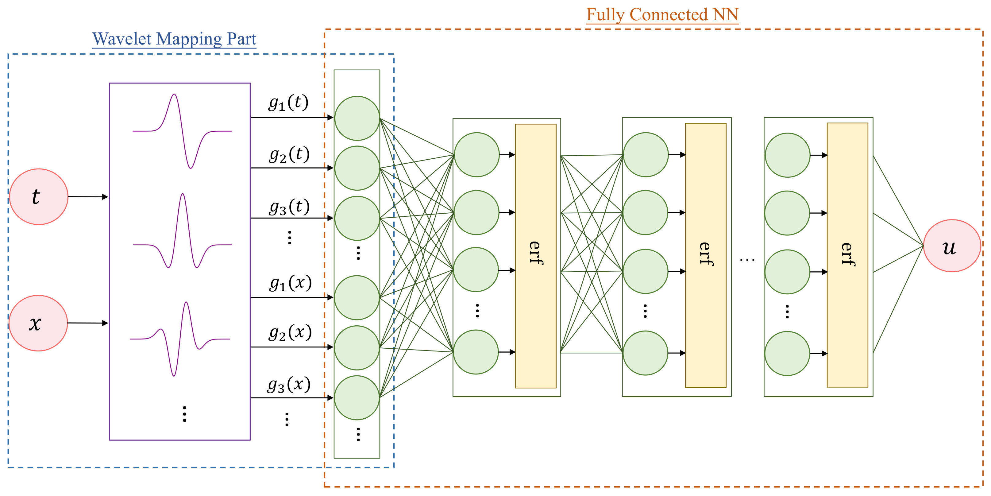
In this section, the basic architecture and the proposed algorithm for solving PDEs are described in detail. Figure 1 shows the structure of DWNN, which is composed of input layer, wavelet expansion layer, fully connected layers and output layer. Specifically, the number of nodes in the input layer is determined by the number of variables. The functional expansion layer is based on a family of wavelets. This is followed by a fully connected neural network. The DWNN model is composed of two modules: one is the wavelet-mapping part and the other is the fully connected part.

2.1. Wavelet Mapping Part

In first part, we map the input data to a higher-dimensional feature space using the family of wavelets. Then, the enhanced pattern is fed into the deep feedforward neural network as new input vectors.

Here, we choose the family of vanishing momentum wavelets (VMWs) [32] for expanding:

$$g_n\left(x\right) = {(-1)}^{n+1}{\displaystyle \frac{d^n}{d{x}^n}}{e}^{-x^2/2},n > 0$$

(1)

where $g_n\left(x\right)$ denotes the n-th wavelets. The first two of VMWs are known as

$$g_1\left(x\right) = -x{e}^{-x^2/2},$$

(2)

$$g_2\left(x\right) = (1 - x^2)e^{-x^2/2}.$$

(3)

The higher-order VMWs can be calculated by Formula (1):

$$g_3\left(x\right) = (3x - x^3)e^{-x^2/2},$$

(4)

$$g_4\left(x\right) = (6x^2 - x^4 - 3)e^{-x^2/2},$$

(5)

$$g_5\left(x\right) = (10x^3 - x^5 - 15x)e^{-x^2/2},$$

(6)

$$g_6\left(x\right) = (15x^4 - x^6 - 45x^2 + 15)e^{-x^2/2}.$$

(7)

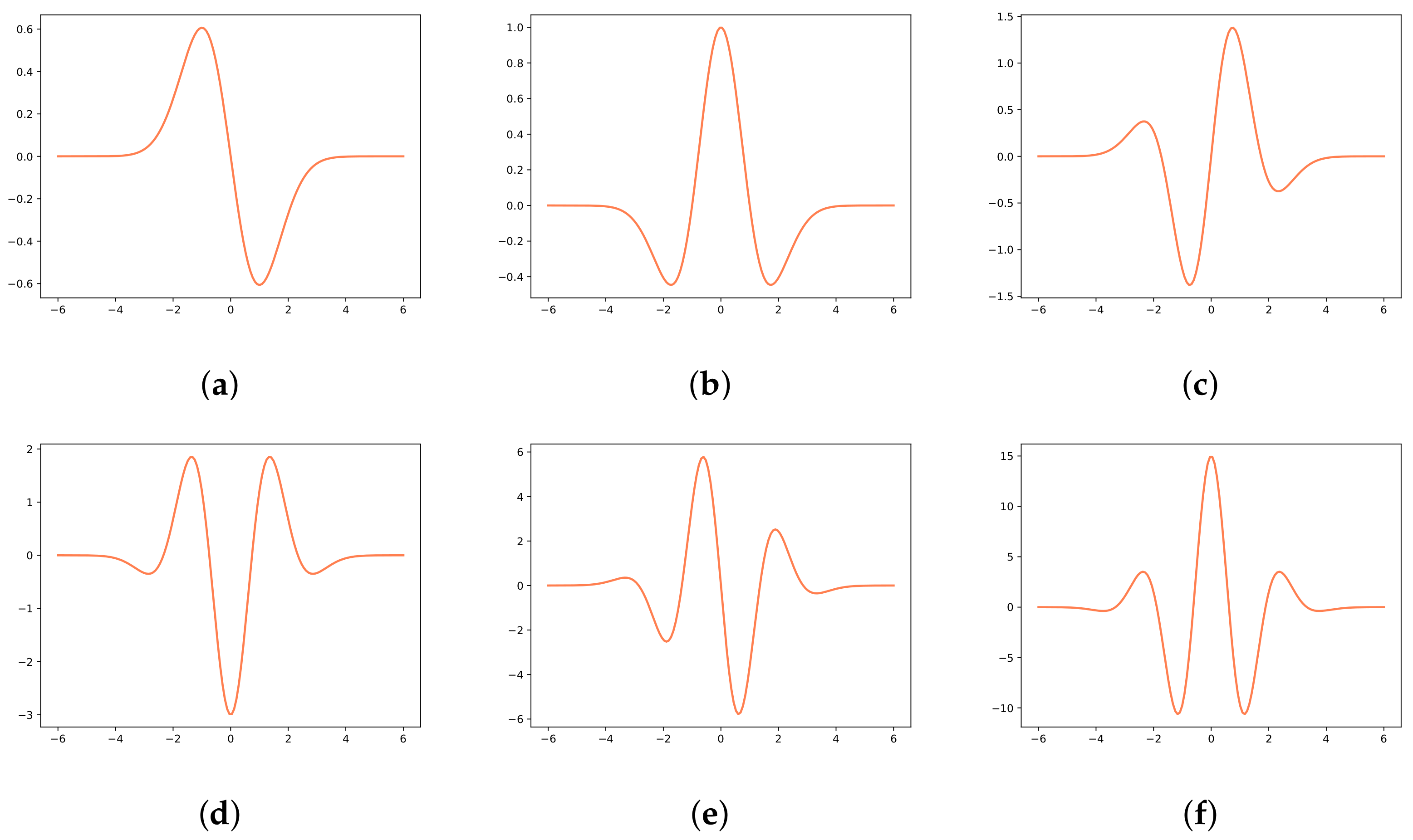
Vanishing momentum wavelets possess a number of significant properties, such as being continuous and differentiable. Moreover, odd-order derivative is an odd function while the even-order derivative is an even function. Both of them are smooth wavelets. Figure 2 presents the waveforms of vanishing momentum wavelets. In practice, the intricate nonlinear behavior of some equations is hard to capture accurately [24]. Hence, we introduce wavelets to deep architecture because wavelet transform can effectively extract more details from the input data and fully highlight some features of the data. Then, around singularities or jumps, the proposed method will make more accurate approximations.

Let $X = (t,x_1,x_2,x_3,\dots ,x_m)$ as the input pattern, then the enhanced pattern is obtained by using the family of vanishing momentum wavelets as

$$[g_1\left(t\right),g_2\left(t\right),\dots ,g_n\left(t\right);g_1\left(x_1\right),g_2\left(x_1\right),\dots ,g_n\left(x_1\right);\dots ;g_1\left(x_m\right),g_2\left(x_m\right),\dots ,g_n\left(x_m\right)].$$

(8)

Thus, the m-dimensional input pattern is mapped to the enhanced n-dimensional pattern ($n > m$). Figure 1 presents the architecture of DWNN model, where $m = 1$, $n = 3$.

2.2. Fully Connected Neural Network

A fully connected neural network is a kind of fundamental artificial neural network. In this network, all neurons are fully connected between adjacent layers. Supposing an L-layer fully connected neural network, the first layer $l = 0$ is the input layer and the last layer $l = L - 1$ is the output layer. Several layers, $0 < l < L - 1$, are called hidden layers. Each hidden layer in the neural network receives the output $x^{l-1}$ from the previous layer:

$${\mathcal{L}}_l\left(x^{l-1}\right) = w^l{x}^{l-1} + b^l.$$

(9)

Then, the nonlinear activation $\sigma (·)$ is imposed to the above vector to become a new input sending to the next layer:

$$x^l = \sigma \left({\mathcal{L}}_l\left(x^{l-1}\right)\right).$$

(10)

Therefore, the information from the input layer is transmitted to the last layer through forward propagation. The final representation of neural network is as follows

$$u_{\theta }\left(x\right) = ({\mathcal{L}}_l \circ \sigma \circ {\mathcal{L}}_{l-1} \circ \cdots \circ \sigma \circ {\mathcal{L}}_1)\left(x\right)$$

(11)

where $\theta = {\{w^l,b^l\}}_{l=1}^L$ is the parameter set and operator ∘ denotes composition operator.

The optimal approximation performance of the network is obtained by minimizing the cost function to a certain tolerance or up to a specified iterations to find the optimum of weights (w) and biases (b). Specifically, we aim to obtain

$$w^{*} = \underset{w\in \theta }{argmin}\left(J\left(w\right)\right)$$

(12)

$$b^{*} = \underset{b\in \theta }{argmin}\left(J\left(b\right)\right)$$

(13)

where $J\left(\theta \right)$ is the cost function. Any optimization method can be used to try to solve this minimization problem. The Newton method is a common optimization method that needs to calculate the second derivative of the objective function, that is, the Hessian matrix. If the Hessian matrix is dense, each iteration requires a large amount of computation and storage space. Moreover, the Newton method is not really robust since the Hessian matrix cannot be guaranteed to always be positive definite. The quasi-Newton method introduces the approximate matrix of the Hessian matrix. The approximate matrix is positive definite, so the algorithm always searches in the direction of the optimal value. However, the computational and storage overhead is still large when the approximate matrix becomes dense. The L-BFGS-B algorithm [33] is an improvement of the quasi-Newton algorithm, which has a small overhead per iteration and fast execution speed. The basic idea is to only save and use the curvature information of the most recent m iterations to construct an approximate matrix of the Hessian matrix. After each iteration, the oldest curvature information is deleted and the newest curvature information is saved. Here, we use L-BFGS-B method [33] to iteratively update the parameter set.

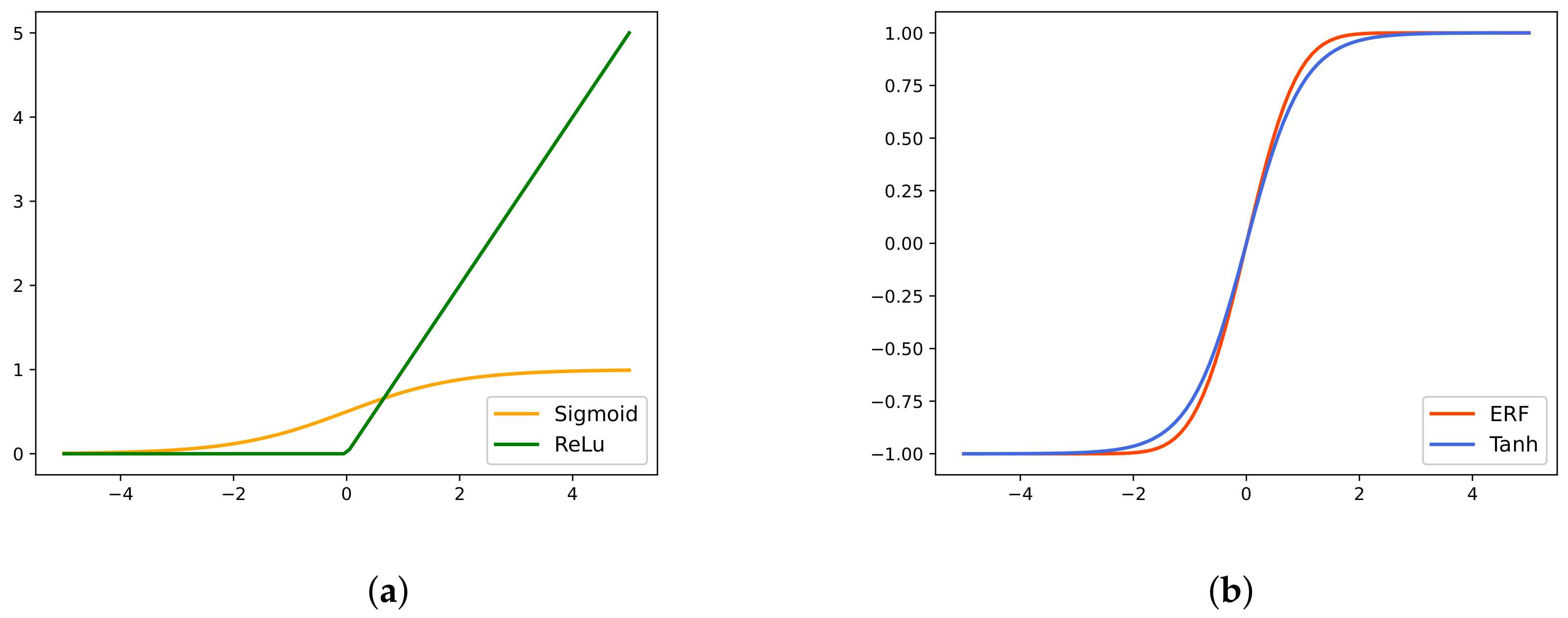
Actually, in the training process of network, the activation function is of great importance because the optimization parameter set depends on the derivative of cost function, which in turn relies on the activation function. The most common activation functions include sigmoid, ReLu, tanh, etc. Figure 3a presents a schematic diagram of sigmoid and ReLu function, from which we see that the output value of sigmoid and ReLu function is not symmetrical about the zero point. Here, we obviously do not want the value obtained by the next neuron to be positive at all times. Figure 3b presents a schematic diagram of tanh and Gaussian error function. The output value of tanh function is symmetric about zero, but the gradient is smooth. Therefore, we find a function whose output value is symmetric about zero, continuous, differentiable, and has a steeper gradient, namely, the Gaussian error function, as the activation function. Under this setting, the convergence rate of the model is accelerated. Gaussian error function is derived from measure theory, which is a special function and broadly applied in probability theory, statistics, etc. [34]. The Gaussian error function with independent variable x is defined as

$$erf\left(x\right) = {\displaystyle \frac{2}{\sqrt{\pi }}}{\int }_0^x{e}^{-{\eta }^2}d\eta .$$

(14)

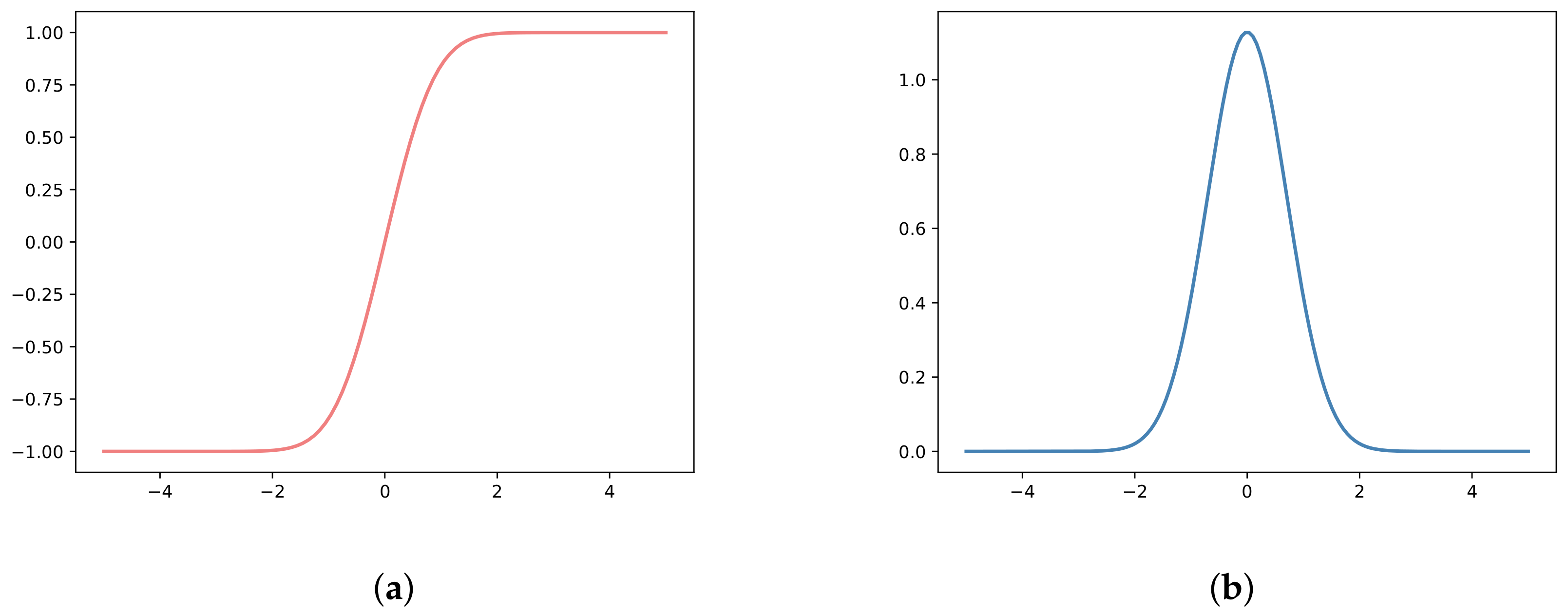
Figure 4a shows a schematic of the Gaussian error function separately. The derivative of Gaussian error function is presented in Figure 4b. It is obvious that the output of Gaussian error function is zero-centered, and the gradient is steep, which accelerates the convergence rate of the model.

The universal approximation theorem [35] states that, for any given tolerance $ϵ$, a DWNN model can be trained such that the resulting approximation error is less than that tolerance $ϵ$. George et al. [36,37] generalize this theorem and present the systematic study of quantitative error bounds. In DWNN model, we apply the wavelet transform to the input coordinates of the input side before fully connected network for multi-scale projection. Then, the lower-dimensional input is mapped to higher-dimensional feature space with no demands on the data. Therefore, the error is still bound by optimization error.

2.3. Loss Function and Algorithm

Assume a PDE given by

$$\left\{\begin{array}{c}{\displaystyle \frac{\partial }{\partial t}}u(t,\mathit{x}) = \mathcal{L}u(t,\mathit{x}),\mathit{x} \in \mathsf{\Omega },t \in [0,T],\hfill \\ u(0,\mathit{x}) = I\left(\mathit{x}\right),\mathit{x} \in \mathsf{\Omega },\hfill \\ u(t,\mathit{x}) = B(t,\mathit{x}),\mathit{x} \in \partial \mathsf{\Omega },t \in [0,T],\hfill \end{array}\right.$$

(15)

where $\mathcal{L}$ represents differential operator and $\partial \mathsf{\Omega }$ denotes the boundary of computational domain $\mathsf{\Omega } \subset {\mathbb{R}}^d$. Initial and boundary conditions are already known. What we need to approximate is $u(t,\mathit{x})$. In PINN [24], $f(t,\mathit{x})$ is defined by the left-hand-side of Equation (15):

$$f(t,\mathit{x}): = {\displaystyle \frac{\partial }{\partial t}}u(t,\mathit{x}) - \mathcal{L}u(t,\mathit{x}),$$

(16)

and we can obtain $f(t,\mathit{x})$ using automatic differentiation [38]. The parameters between $f(t,\mathit{x})$ and $u(t,\mathit{x})$ are shared. We seek to approximate the unknown function $u(t,\mathit{x})$ utilizing the defined model with parameters. The goal is to find the optimum of parameter set $\theta$ that minimizes the properly defined cost function. To be more specific, the cost function $J\left(\theta \right)$ is written as

$$J\left(\theta \right) = MS{E}_f + MS{E}_{ic} + MS{E}_{bc} + \alpha MS{E}_{domain},$$

(17)

where MSE is defined as

$$MS{E}_f = \frac{1}{N_f}\sum _{i=1}^{N_f}f{(t_f^i,{\mathit{x}}_{\mathit{f}}^{\mathit{i}})}^2,$$

(18)

$$MS{E}_{ic} = \frac{1}{N_{ic}}\sum _{i=1}^{N_{ic}}{(u(t_{ic}^i,{\mathit{x}}_{\mathit{ic}}^{\mathit{i}}) - u^i)}^2,$$

(19)

$$MS{E}_{bc} = \frac{1}{N_{bc}}\sum _{i=1}^{N_{bc}}{(u(t_{bc}^i,{\mathit{x}}_{\mathit{bc}}^{\mathit{i}}) - u^i)}^2,$$

(20)

$$MS{E}_{domain} = \frac{1}{N_{domain}}\sum _{i=1}^{N_{domain}}{(u(t_{domain}^i,{\mathit{x}}_{\mathit{domain}}^{\mathit{i}}) - u^i)}^2.$$

(21)

Here, ${\{t_f^i,{\mathit{x}}_{\mathit{f}}^{\mathit{i}}\}}_{i=1}^{N_f}$ denotes the residual training points on $f(t,\mathit{x})$, ${\{t_{ic}^i,{\mathit{x}}_{\mathit{ic}}^{\mathit{i}},u^i\}}_{i=1}^{N_{ic}}$ represents the initial points on $u(t,\mathit{x})$, ${\{t_{bc}^i,{\mathit{x}}_{\mathit{bc}}^{\mathit{i}},u^i\}}_{i=1}^{N_{bc}}$ denotes the boundary points on $u(t,\mathit{x})$, and ${\{t_{domain}^i,{\mathit{x}}_{\mathit{domain}}^{\mathit{i}},u^i\}}_{i=1}^{N_{domain}}$ denotes the interior training points in the domain of $u(t,\mathit{x})$. $N_f$ refers to the number of collocation points, $N_{ic}$/$N_{bc}$ corresponds to the number of initial/boundary data, and $N_{domain}$ represents the number of observations. The coefficient $\alpha$ depends on the governing equation itself and is usually set to 0 or 1. $J\left(\theta \right)$ evaluates the degree of inconsistency between the network model and the true value. Concretely, the first term serves as a penalty constraining the solution space, the second and third terms are regarded as the constraints of initial and boundary conditions, respectively. The last depicts the deviation between the output of neural network and ground truth. We usually set $\alpha$ to 1 to rectify the model by utilizing the last term when dealing with the problems with shock wave and interface. If the solution of equation is continuous, this term degenerates, which means $\alpha$ equals zero. In this paper, we use L-BFGS-B method [33] that has faster convergence speed and less memory cost to optimize all target loss functions. The resulting algorithm, termed as deep wavelet neural network, is summarized in Algorithm 1.

Algorithm 1 Deep Wavelet Neural Network (DWNN) for solving partial differential equations.

Input: Collocation points ${\{t_f^i,{\mathit{x}}_{\mathit{f}}^{\mathit{i}}\}}_{i=1}^{N_f}$; Initial training data ${\{t_{ic}^i,{\mathit{x}}_{\mathit{ic}}^{\mathit{i}},u^i\}}_{i=1}^{N_{ic}}$; Boundary training data ${\{t_{bc}^i,{\mathit{x}}_{\mathit{bc}}^{\mathit{i}},u^i\}}_{i=1}^{N_{bc}}$; Observations ${\{t_{domain}^i,{\mathit{x}}_{\mathit{domain}}^{\mathit{i}},u^i\}}_{i=1}^{N_{domain}}$. Output: Neural network predicted solution $u(t,\mathit{x})$. 1: Construct the architecture of neural network with wavelet layer and parameter set $\theta$; 2: Specify the training set $N_f$,$N_{ic}$,$N_{bc}$,$N_{domain}$ for collocation points, initial, boundary and domain points; 3: Make DWNN wavelet-based expansion layer of input data as $$[g_1\left(t\right),g_2\left(t\right),\dots ,g_n\left(t\right);g_1\left(x_1\right),g_2\left(x_1\right),\dots ,g_n\left(x_1\right);\dots ;g_1\left(x_m\right),g_2\left(x_m\right),\dots ,g_n\left(x_m\right)];$$ 4: Specity the loss function with the coefficient $\alpha$ by adjusting the sum of PDEs residuals, initial/boundary conditions and observations residuals; 5: Train the neural network to find the best parameters by minimizing the loss function with L-BFGS-B optimization method; 6: return $u(t,\mathit{x})$;

3. Numerical Results

We consider various forms of partial differential equations to illustrate the validity and robustness of the proposed method in this section. We evaluate the accuracy of numerical solution by relative $L^2$ error and $L^{\infty }$ error. The results demonstrate that the predicted result of deep wavelet neural network is more accurate. In Section 3.1, five equations are shown to validate the effectiveness of the proposed algorithm in one-dimensional space, and in Section 3.2, three examples are given to verify the correctness of our method in two-dimensional space. Lastly, in Section 3.3, two equations are shown to demonstrate the reliability and generalization ability of the proposed method in high-dimensional space.

3.1. One-Dimensional Equations

In this subsection, we take five different one-dimensional equations, these being the Schrödinger equation, carburizing equation, Klein-Gordon equation, Burgers equation and Allen-Cahn equation, to show the stability and reliability of our method.

3.1.1. Schrödinger Equation

In order to demonstrate the validity of our method for handling periodic boundary conditions, complex-valued functions and diverse kinds of nonlinearities in the PDEs [39], the Schrödinger equation is introduced in this subsection. The Schrödinger equation is a fundamental assumption in quantum mechanics proposed by the Austrian physicist Schrodinger [40]. It describes the motion of microscopic particles and each microscopic system has a corresponding equation. In one-dimensional space, the Schrödinger equation with periodic boundary conditions reads as

$$\left\{\begin{array}{c}i{h}_t + 0.5h_{xx} + {\left|h\right|}^{2}h = 0,t \in [0,\pi /2],x \in [-5,5],\hfill \\ h(0,x) = 2sech\left(x\right),\hfill \\ h(t,-5) = h(t,5),\hfill \\ h_x(t,-5) = h_x(t,5).\hfill \end{array}\right.$$

(22)

In this case, we use seven wavelets in the wavelet expansion layer and the following fully connected neural network is considered to be four hidden layers with 100 neurons per hidden layer. Gaussian error function is taken for the activation function. The $f(t,x)$ is obtained from the left-hand-side of Equation (22)

$$f := i{h}_t + 0.5h_{xx} + {\left|h\right|}^{2}h.$$

(23)

Actually, $h(t,x)$ is the complex-valued solution that contains a real part and imaginary part. Supposing $u(t,x)$ represents the real part and $v(t,x)$ denotes the imaginary part, the complexed-valued solution $h(t,x)$ is rewritten as $h(t,x) = \left[u\right(t,x),v(t,x\left)\right]$. Therefore, the neural network is multi-output because two units are needed to completely represent the entire solution. The cost function $J\left(\theta \right)$ is composed of three terms:

$$J\left(\theta \right) = MS{E}_f + MS{E}_0 + MS{E}_b,$$

(24)

where

$$MS{E}_f = \frac{1}{N_f}\sum _{i=1}^{N_f}{\left|f(t_f^i,x_f^i)\right|}^2,$$

(25)

$$MS{E}_0 = \frac{1}{N_0}\sum _{i=1}^{N_0}{|h(0,x_0^i) - h_0^i|}^2,$$

(26)

$$MS{E}_b = \frac{1}{N_b}\sum _{i=1}^{N_b}\left({|h(t_b^i,-5) - h(t_b^i,5)|}^2 + {|h_x(t_b^i,-5) - h_x(t_b^i,5)|}^2\right).$$

(27)

Here, ${\{t_f^i,x_f^i\}}_{i=1}^{N_f}$ specifies the unsupervised points on $f(t,x)$, ${\{x_0^i,h_0^i\}}_{i=1}^{N_0}$ specifies the initial points on $h(t,x)$, and ${\left\{t_b^i\right\}}_{i=1}^{N_b}$ specifies the boundary points on $h(t,x)$.

The training set consists of initial points $N_0 = 50$, boundary points $N_b = 50$, and collocation points $N_f$ = 20,000. All randomly sampled point locations are generated using a Latin Hypercube Sampling strategy [41]. To evaluate the accuracy of this model, we use the dataset from PINN [24]. They used traditional spectral method to simulate this problem. Specifically, Equation (22) is integrated from the initial time $t = 0$ to the final time $t = \pi /2$ using the Chebfun package [42] under the set boundary conditions.

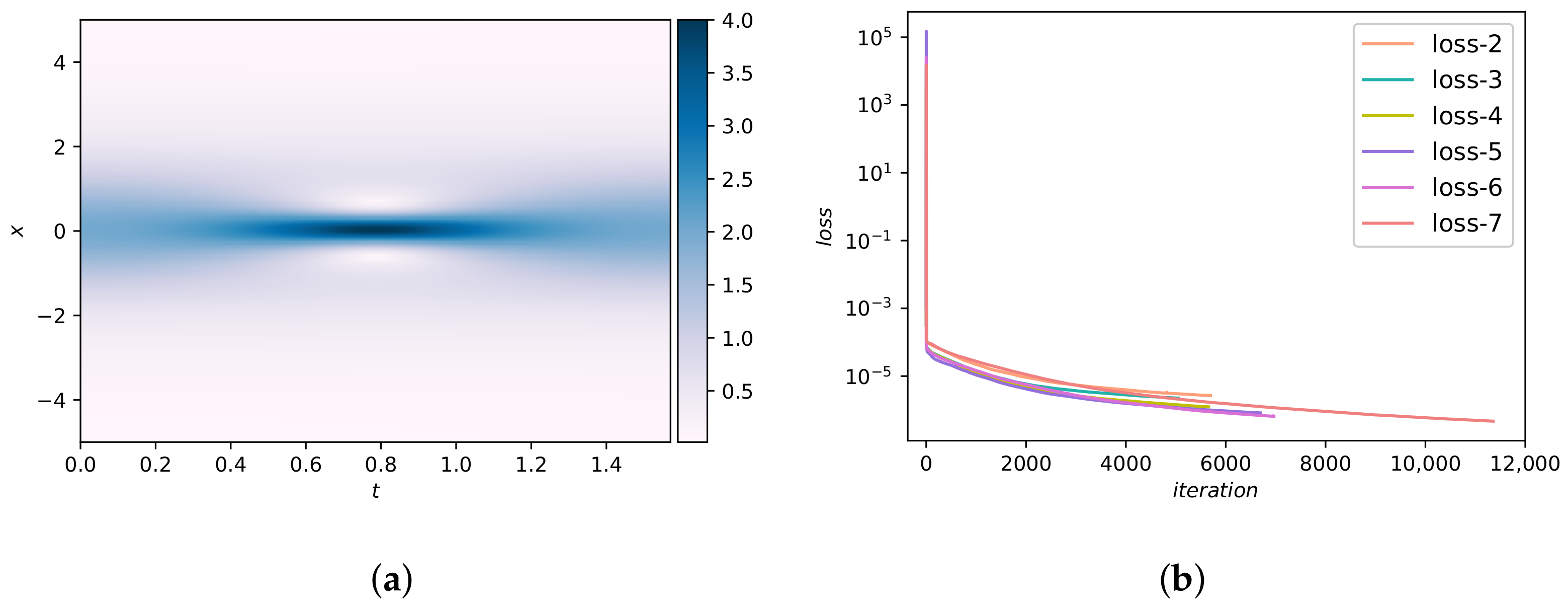
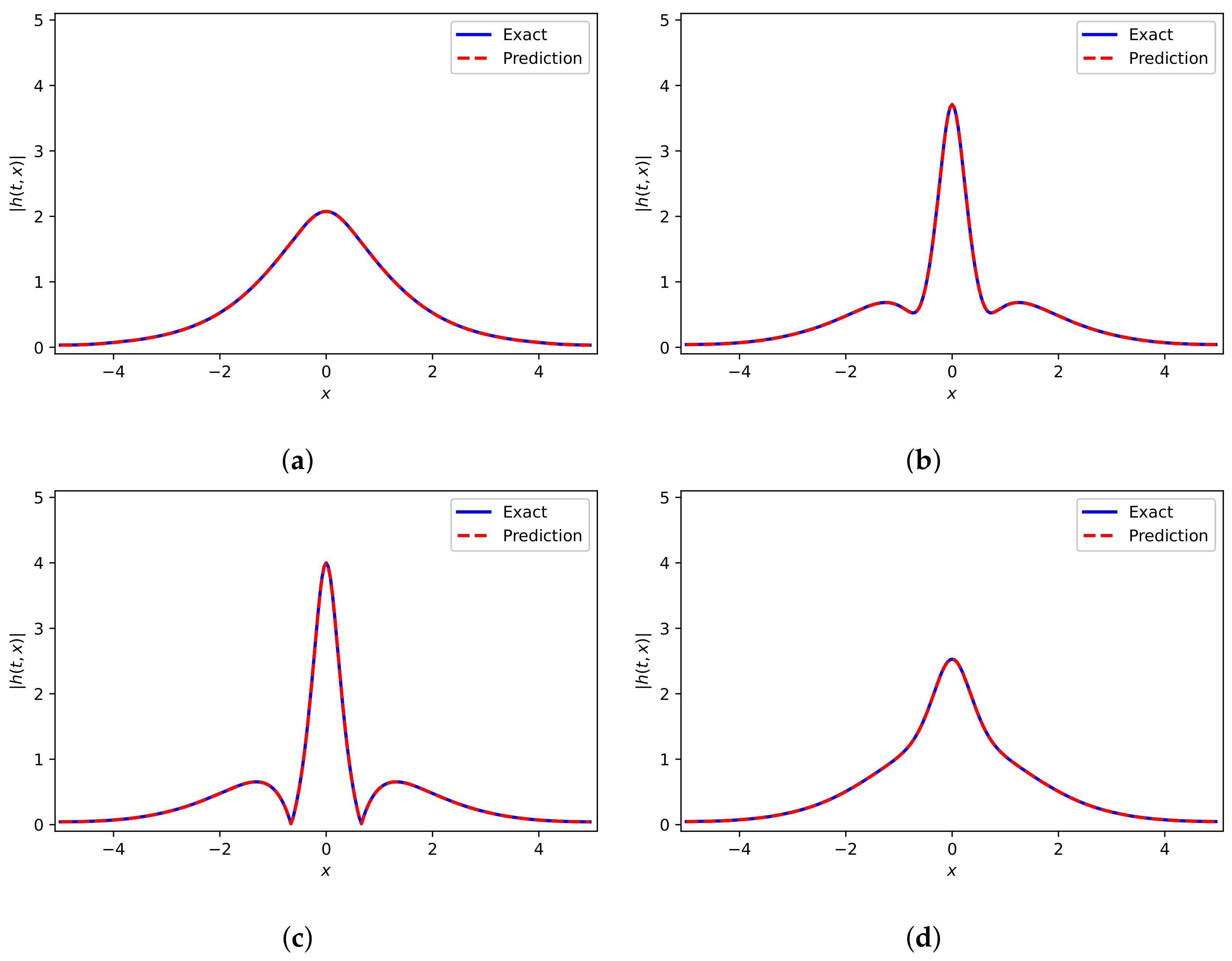
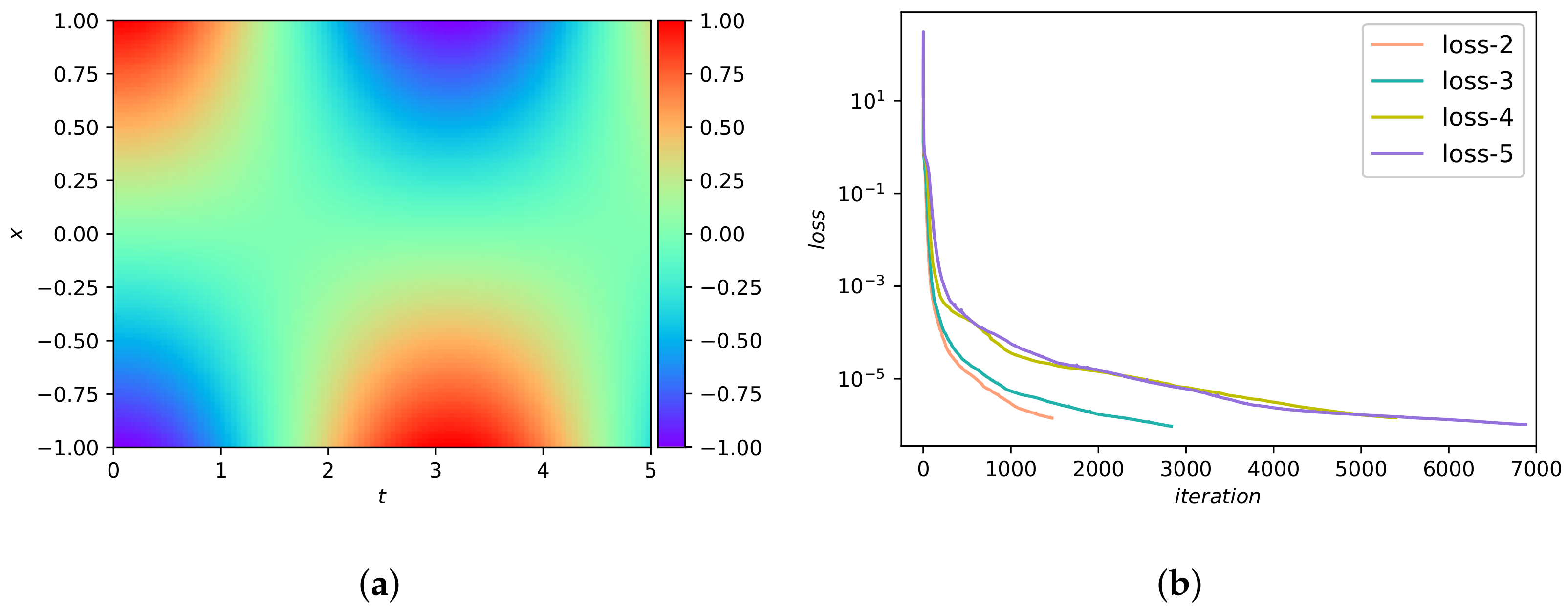
In this example, we first use Adam [43] for 50,000 iterations and then use L-BFGS-B method for optimization. Figure 5a presents the DWNN model predicted solution $\left|h\right(t,x\left)\right|$. It seems that the predicted sulution is coincident with analytical solution. Furthermore, a presentation with regard to the convegence rate of DWNN model for different number of wavelets is shown in Figure 5b. It is seen that the DWNN model using seven wavelets keeps converging until the least, while training is terminated prematurely in other cases to prevent overfitting. The prediction error for this case calculated in the end is $5.04 \times {10}^{-4}$ in the relative $L^2$-norm. It is noted that this prediction error is an order of magnitude smaller than the error previously described using PINN [24]. A detailed assessment of the neural network solution at different temporal snapshots $t = (0.16,0.67,0.79,1.18)$ is reflected in Figure 6. We find that there is a satisfactory agreement of the predicted DWNN solution and exact solution.

To further investigate the capability of the proposed method, the following systematic studies are carried out to quantify the predictive accuracy for different number of wavelets as well as for different hidden layers.

Table 1. The $L^2$ errors and $L^{\infty }$ errors for 1D Schrödinger.

${\mathit{L}}^2$ Error		VMWs	$\mathit{l} = 1$	$\mathit{l} = 2$	$\mathit{l} = 3$	$\mathit{l} = 4$
		2	$2.47 \times {10}^{-1}$	$1.99 \times {10}^{-3}$	$1.24 \times {10}^{-3}$	$1.18 \times {10}^{-3}$
		3	$3.25 \times {10}^{-2}$	$1.25 \times {10}^{-3}$	$1.15 \times {10}^{-3}$	$1.03 \times {10}^{-3}$
	DWNN with Equation (22)	4	$4.34 \times {10}^{-2}$	$9.49 \times {10}^{-4}$	$9.96 \times {10}^{-4}$	$9.02 \times {10}^{-4}$
		5	$7.66 \times {10}^{-3}$	$8.52 \times {10}^{-4}$	$8.68 \times {10}^{-4}$	$8.00 \times {10}^{-4}$
		6	$2.50 \times {10}^{-2}$	$7.28 \times {10}^{-4}$	$6.49 \times {10}^{-4}$	$6.03 \times {10}^{-4}$
		7	$1.73 \times {10}^{-2}$	$6.88 \times {10}^{-4}$	$6.24 \times {10}^{-4}$	$5.04 \times {10}^{-4}$
	PINN	-	$2.60 \times {10}^{-1}$	$1.54 \times {10}^{-3}$	$1.23 \times {10}^{-3}$	$1.11 \times {10}^{-3}$
${\mathit{L}}^{\infty }$ Error
		2	$3.19 \times {10}^{-1}$	$2.47 \times {10}^{-3}$	$1.65 \times {10}^{-3}$	$1.59 \times {10}^{-4}$
		3	$4.46 \times {10}^{-2}$	$1.39 \times {10}^{-3}$	$1.57 \times {10}^{-3}$	$1.50 \times {10}^{-3}$
	DWNN with Equation (22)	4	$5.92 \times {10}^{-2}$	$1.40 \times {10}^{-3}$	$1.47 \times {10}^{-3}$	$1.44 \times {10}^{-3}$
		5	$1.06 \times {10}^{-2}$	$1.36 \times {10}^{-3}$	$1.40 \times {10}^{-3}$	$1.27 \times {10}^{-3}$
		6	$3.51 \times {10}^{-2}$	$1.27 \times {10}^{-3}$	$1.28 \times {10}^{-3}$	$1.19 \times {10}^{-3}$
		7	$2.37 \times {10}^{-2}$	$1.28 \times {10}^{-3}$	$1.18 \times {10}^{-3}$	$1.12 \times {10}^{-3}$
	PINN	-	$3.38 \times {10}^{-1}$	$1.78 \times {10}^{-3}$	$1.52 \times {10}^{-3}$	$1.54 \times {10}^{-3}$

summarizes the $L^{\infty }$ errors and $L^2$ errors with respect to different numbers of wavelets (VMWs) and different numbers of hidden layers (l), while keeping 100 hidden neurons fixed in each hidden layer. As expected, the predictive accuracy increases as the number of wavelets and hidden layers increase. To illustrate the insensitivity of the DWNN model to noise, we perform a systematic study with respect to the noise corruption levels in one-dimensional Schrödinger experiment. The results are listed in

Table 2. The relative $L^2$ errors with respect to different noise levels for 1D Schrödinger.

Noise Level	0% Noise	1% Noise	10% Noise	15% Noise
Relative $L^2$ error	$5.04 \times {10}^{-4}$	$5.18 \times {10}^{-3}$	$5.49 \times {10}^{-2}$	$7.25 \times {10}^{-2}$

, from which we observe that the proposed approach is robust.

3.1.2. Carburizing Diffusion Equation

To demonstrate the ability of the method presented in this paper to solve realistic problems, we consider the carburzing diffusion model. Carburizing is a chemical heat-treatment process, which is widely used in low carbon/alloy steel. The specific method is to put the workpiece into the active carburizing medium and obtain the high carbon in surface layer by heating and holding. The carburizing process can make the surface of a carburized workpiece obtain higher hardness, so as to improve the wear resistance [44,45]. The form of the nonlinear carburizing diffusion equation is

$$\left\{\begin{array}{c}{c}_t = {\left(D\left(c\right)c_x\right)}_x,t \in [0,T],x \in [a,b],\hfill \\ c(0,x) = c_0\left(x\right),\hfill \\ c(t,a) = c_l,c(t,b) = c_r,\hfill \end{array}\right.$$

(28)

where c denotes the carbon concentration and $D\left(c\right)$ denotes the diffusion coefficient that depends on the concentration. The diffusion coefficient dynamically varies due to external factors such as temperature in practical problems. In this experiment, we consider a variable coefficient $D\left(c\right) = cos\left(c\right)$. A source term added is given by

$$g(t,x) = sin(e^{-dt}sinx)e^{-2dt}{cos}^{2}x - d{e}^{-dt}sinx + cos(e^{-dt}sinx)e^{-dt}sinx.$$

(29)

Then the corresponding exact solution is $c(t,x) = e^{-dt}sinx$. The computing domain is set to $x \in [-\pi ,\pi ]$, $t \in [0,1]$. The case $d = 0.5$. We compute the above problem with homogeneous Dirichlet boundary condition. The network structure consists of a wavelet expansion layer with five wavelets and a fully connected part with four hidden layers. Each hidden layer contains 20 neurons and a Gaussian error function. The $f(t,x)$ is obtained from Equation (28)

$$f: = c_t - {\left(D\left(c\right)c_x\right)}_x.$$

(30)

The cost function $J\left(\theta \right)$ is composed of three parts: $MS{E}_f$, $MS{E}_{ic}$, $MS{E}_{bc}$. For brevity, we use $MS{E}_c$ to characterize the initial and boundary conditions. Therefore, the cost function is given by

$$J\left(\theta \right) = MS{E}_f + MS{E}_c,$$

(31)

where

$$MS{E}_f = \frac{1}{N_f}\sum _{i=1}^{N_f}{\left|f(t_f^i,x_f^i)\right|}^2,$$

(32)

$$MS{E}_c = \frac{1}{N_c}\sum _{i=1}^{N_c}{|c(t_c^i,x_c^i) - c^i|}^2.$$

(33)

Given a set of 100 initial/boundary data and 10,000 collocation points, we obtain the latent solution $c(t,x)$ by training the DWNN model. The predicted solution $c(t,x)$ of deep wavelet neural network is shown in Figure 7a, and we observe that our results show great agreement with the exact results [46]. The curves of loss functions associated to the number of wavelets are plotted in Figure 7b. From Figure 7b, we find that employing five wavelets can achieve the minimum loss with fewer iterations. The relative $L^2$ error measured is $8.76 \times {10}^{-5}$. Figure 8 provides a more detailed visual comparison at unequal temporal snapshots $t = (0.25,0.55,0.75,1.0)$, respectively. It is clearly seen that the experimental solution coincides with the analytical solution.

To further verify the validity of the proposed method, we carry out a systematic study with regard to different number of VMWs and different number of hidden layers, while the number of hidden neurons are fixed to 20 per hidden layer. The resulting $L^{\infty }$ errors and $L^2$ errors are given in

Table 3. The $L^2$ errors and $L^{\infty }$ errors for 1D carburizing diffusion equation.

${\mathit{L}}^2$ Error		VMWs	$\mathit{l}=2$	$\mathit{l}=4$	$\mathit{l}=6$	$\mathit{l}=8$
		2	$4.60 \times {10}^{-4}$	$2.75 \times {10}^{-4}$	$2.88 \times {10}^{-4}$	$3.20 \times {10}^{-4}$
		3	$4.78 \times {10}^{-4}$	$3.79 \times {10}^{-4}$	$2.65 \times {10}^{-4}$	$1.32 \times {10}^{-4}$
	DWNN with Equation (28)	4	$3.54 \times {10}^{-4}$	$3.73 \times {10}^{-4}$	$3.42 \times {10}^{-4}$	$3.64 \times {10}^{-4}$
		5	$3.01 \times {10}^{-4}$	$8.76 \times {10}^{-5}$	$1.27 \times {10}^{-4}$	$3.20 \times {10}^{-4}$
		6	$2.97 \times {10}^{-4}$	$3.25 \times {10}^{-4}$	$2.94 \times {10}^{-4}$	$2.24 \times {10}^{-4}$
		7	$1.18 \times {10}^{-3}$	$5.22 \times {10}^{-4}$	$5.47 \times {10}^{-4}$	$3.02 \times {10}^{-4}$
	PINN	-	$1.33 \times {10}^{-3}$	$1.28 \times {10}^{-3}$	$1.02 \times {10}^{-3}$	$9.59 \times {10}^{-4}$
${\mathit{L}}^{\infty }$ Error
		2	$1.26 \times {10}^{-3}$	$1.51 \times {10}^{-3}$	$6.70 \times {10}^{-4}$	$8.29 \times {10}^{-4}$
		3	$9.78 \times {10}^{-4}$	$1.26 \times {10}^{-3}$	$6.50 \times {10}^{-4}$	$7.82 \times {10}^{-4}$
	DWNN with Equation (28)	4	$8.61 \times {10}^{-4}$	$1.37 \times {10}^{-3}$	$9.74 \times {10}^{-4}$	$1.07 \times {10}^{-3}$
		5	$8.49 \times {10}^{-4}$	$4.29 \times {10}^{-4}$	$5.54 \times {10}^{-4}$	$8.16 \times {10}^{-4}$
		6	$8.31 \times {10}^{-4}$	$1.33 \times {10}^{-3}$	$1.03 \times {10}^{-3}$	$7.83 \times {10}^{-4}$
		7	$3.46 \times {10}^{-3}$	$1.21 \times {10}^{-3}$	$1.36 \times {10}^{-3}$	$1.28 \times {10}^{-3}$
	PINN	-	$3.81 \times {10}^{-3}$	$2.34 \times {10}^{-3}$	$2.47 \times {10}^{-3}$	$2.51 \times {10}^{-3}$

. We easily find that the prediction error reduces when the number of wavelets increase in general. It seems that the proposed methodology effectively improves the predictive accuracy. Additionally, by using wavelet expansions, the system becomes fairly stable so that the prediction error can remain at levels of ${10}^{-4}$ with fewer hidden layers.

3.1.3. Klein-Gordon Equation

In this part, we consider a Klein-Gordon equation that is second order in both time and space. The Klein-Gordon equation is a fundamental equation in relativistic quantum mechanics and quantum field theory. It is a special relativistic form of the Schrodinger equation used to describe particles with zero spin. Moreover, the Klein-Gordon equation arises in many scientific areas, such as condensed matter physics [47], nonlinear wave equations [48], quantum field theory [49], etc. The form of an inhomogeneous Klein-Gordon equation is as follows

$$u_{tt} + \alpha \Delta u + N\left(u\right) - h(t,x) = 0,t > 0,x \in [-1,1],$$

(34)

where the initial and boundary conditions are both derive from analytical solution $u(t,x) = xcos\left(t\right)$. $\Delta$ denotes the Laplacian operator which acts on the space variables only. $N\left(u\right) = \beta u + \gamma u^k$ and $\alpha$, $\beta$, $\gamma$ are all constants.

We set the computational domain $x \in [-1,1]$. In addition, we consider $\alpha$, $\beta$ and $\gamma$ to −1, 0, 1, respectively. k is set to 2. Further, the term $h(t,x)$ is given by $h(t,x) = -xcos\left(t\right) + x^{2}co{s}^{2}t$. The deep architecture used for the computation contains wavelet expansion layer with five VMWs and five hidden layers with 50 neurons per layer. Gaussian error function is assumed to the activation function. The $f(t,x)$ is obtained from the left-hand side of Equation (34)

$$f := u_{tt} + \alpha \Delta u + N\left(u\right) - h(t,x).$$

(35)

The optimal parameters are trained by minimizing the cost function $J\left(\theta \right)$

$$MSE = MS{E}_f + MS{E}_u,$$

(36)

where

$$MS{E}_f = \frac{1}{N_f}\sum _{i=1}^{N_f}{\left|f(t_f^i,x_f^i)\right|}^2,$$

(37)

$$MS{E}_u = \frac{1}{N_u}\sum _{i=1}^{N_u}{|u(t_u^i,x_u^i) - u^i|}^2.$$

(38)

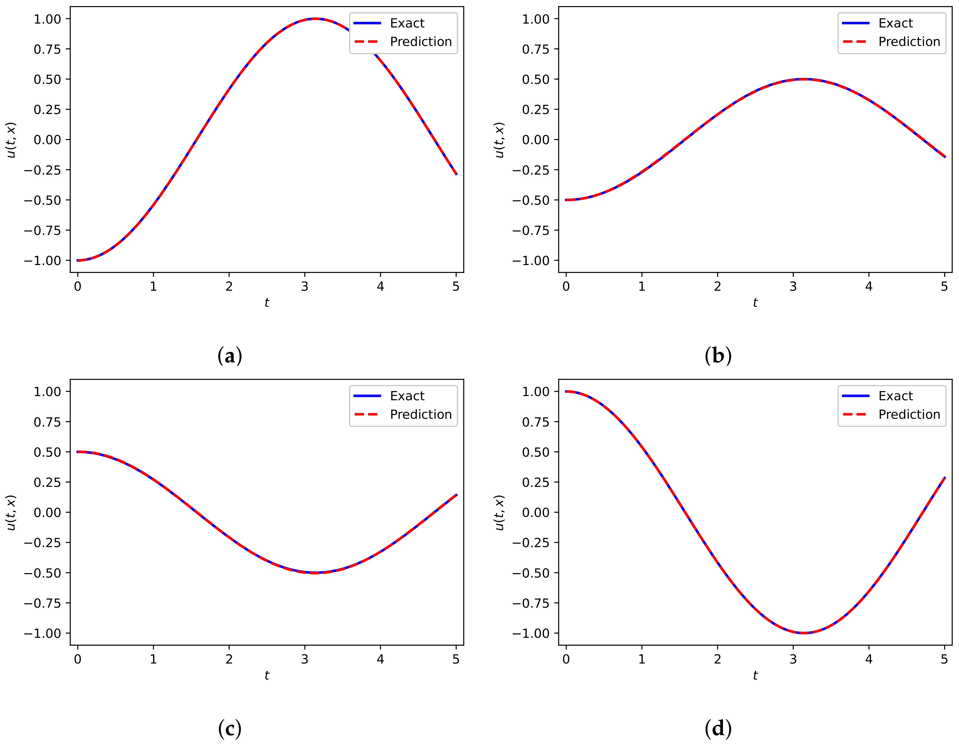
We give a set of 100 randomly chosen initial/boundary data and 10,000 collocation points to train all parameters of neural network. The prediction error is calculated at $3.04 \times {10}^{-3}$ in the relative $L^2$-norm. Figure 9a presents the predicted DWNN solution $u(t,x)$. There is little substantial difference between the predicted results and theorized results [50]. Figure 9b shows the optimization process for the parameters of deep wavelet neural network under a different number of VMWs. We see that using five wavelets has the best performance. A more intuitive assessment of the predicted solution corresponding to four different space points $x = (-1,-0.5,0.5,1)$ is plotted in Figure 10. Coming to the comparison of results, we observe that the simulation results are in great agreement with the exact solution. The $L^{\infty }$ errors and $L^2$ errors according to different number of VMWs and different number of hidden layers are summarized in

Table 4. The $L^2$ errors and $L^{\infty }$ errors for 1D Klein-Gordon.

${\mathit{L}}^2$ Error		VMWs	$\mathit{l}=1$	$\mathit{l}=3$	$\mathit{l}=5$	$\mathit{l}=7$
		2	$5.13 \times {10}^{-2}$	$2.78 \times {10}^{-2}$	$2.62 \times {10}^{-2}$	$2.03 \times {10}^{-2}$
		3	$5.45 \times {10}^{-3}$	$6.57 \times {10}^{-3}$	$4.97 \times {10}^{-3}$	$2.45 \times {10}^{-2}$
	DWNN with Equation (34)	4	$2.40 \times {10}^{-2}$	$1.63 \times {10}^{-2}$	$4.82 \times {10}^{-3}$	$4.50 \times {10}^{-3}$
		5	$4.11 \times {10}^{-2}$	$4.38 \times {10}^{-2}$	$3.04 \times {10}^{-3}$	$4.62 \times {10}^{-3}$
		6	$3.40 \times {10}^{-2}$	$6.41 \times {10}^{-3}$	$1.12 \times {10}^{-2}$	$4.02 \times {10}^{-3}$
		7	$1.54 \times {10}^{-2}$	$1.32 \times {10}^{-2}$	$1.62 \times {10}^{-2}$	$6.82 \times {10}^{-3}$
	PINN	-	$8.08 \times {10}^{-3}$	$9.55 \times {10}^{-3}$	$1.72 \times {10}^{-2}$	$1.55 \times {10}^{-2}$
${\mathit{L}}^{\infty }$ Error
		2	$4.43 \times {10}^{-2}$	$2.32 \times {10}^{-2}$	$2.12 \times {10}^{-2}$	$1.72 \times {10}^{-2}$
		3	$6.09 \times {10}^{-3}$	$5.96 \times {10}^{-3}$	$5.13 \times {10}^{-3}$	$2.00 \times {10}^{-2}$
	DWNN with Equation (34)	4	$2.03 \times {10}^{-2}$	$1.49 \times {10}^{-2}$	$4.89 \times {10}^{-3}$	$4.75 \times {10}^{-3}$
		5	$3.37 \times {10}^{-2}$	$3.70 \times {10}^{-2}$	$3.48 \times {10}^{-3}$	$4.79 \times {10}^{-3}$
		6	$2.97 \times {10}^{-2}$	$7.95 \times {10}^{-3}$	$9.27 \times {10}^{-3}$	$4.64 \times {10}^{-3}$
		7	$2.89 \times {10}^{-2}$	$1.24 \times {10}^{-2}$	$1.71 \times {10}^{-2}$	$9.71 \times {10}^{-3}$
	PINN	-	$8.83 \times {10}^{-3}$	$8.01 \times {10}^{-3}$	$1.60 \times {10}^{-2}$	$1.40 \times {10}^{-2}$

, where the hidden neurons are fixed to 50. From this table, we find that the prediction error declines with increasing number of VMWs until it becomes stable.

3.1.4. Burgers Equation

The Burgers equation is a basic equation in various fields of applied mathematics, such as gas dynamics, fluid mechanics [51], and traffic flow [52]. In 1915, the Burgers equation was first proposed by Harry Bateman [53]. It is a nonlinear partial differential equation that simulates the propagation and reflection of shock waves. Since it is hard for traditional numerical methods to capture strong shock waves, we solve this equation with our method. In one-dimensional space, the Burgers equation with Dirichlet boundary conditions is given by

$$\left\{\begin{array}{c}{u}_t + u{u}_x - {\displaystyle \frac{0.01}{\pi }}{u}_{xx} = 0,t \in [0,1],x \in [-1,1],\hfill \\ u(0,x) = -sin\left(\pi x\right),\hfill \\ u(t,-1) = u(t,1) = 0.\hfill \end{array}\right.$$

(39)

We use DWNN model to solve this equation. Therein, five wavelets are used in wavelet expansion layer. The following fully connected neural network is fixed to 8 hidden layers and each hidden layer contains 20 neurons. The $f(t,x)$ is obtained from the left-hand side of Equation (39)

$$f := u_t + u{u}_x - {\displaystyle \frac{0.01}{\pi }}{u}_{xx}.$$

(40)

The value of $f(t,x)$ can be obtained with autodifferentiation. The complicated nonlinear behaviour of the Burgers equation results in the formation of a acuminate internal layer. It is notoriously difficult to solve with traditional numerical methods accurately. So, we add the residual of a handful of observations into cost function. To be specific, the loss function $J\left(\theta \right)$ is expressed as

$$J\left(\theta \right) = MS{E}_f + MS{E}_u + MS{E}_{domain},$$

(41)

where

$$MS{E}_f = \frac{1}{N_f}\sum _{i=1}^{N_f}{\left|f(t_f^i,x_f^i)\right|}^2,$$

(42)

$$MS{E}_u = \frac{1}{N_u}\sum _{i=1}^{N_u}{|u(t_u^i,x_u^i) - u^i|}^2,$$

(43)

$$MS{E}_{domain} = \frac{1}{N_{domain}}\sum _{i=1}^{N_{domain}}{|u(t_{domain}^i,x_{domain}^i) - u^i|}^2.$$

(44)

Here, ${\{t_f^i,x_f^i\}}_{i=1}^{N_f}$ specifies the collocaction points on $f(t,x)$, ${\{t_u^i,x_u^i,u^i\}}_{i=1}^{N_u}$ denotes the initial/boundary points on $u(t,x)$, and ${\{t_{domain}^i,x_{domain}^i,u^i\}}_{i=1}^{N_{domain}}$ represents the interior training points in the domain.

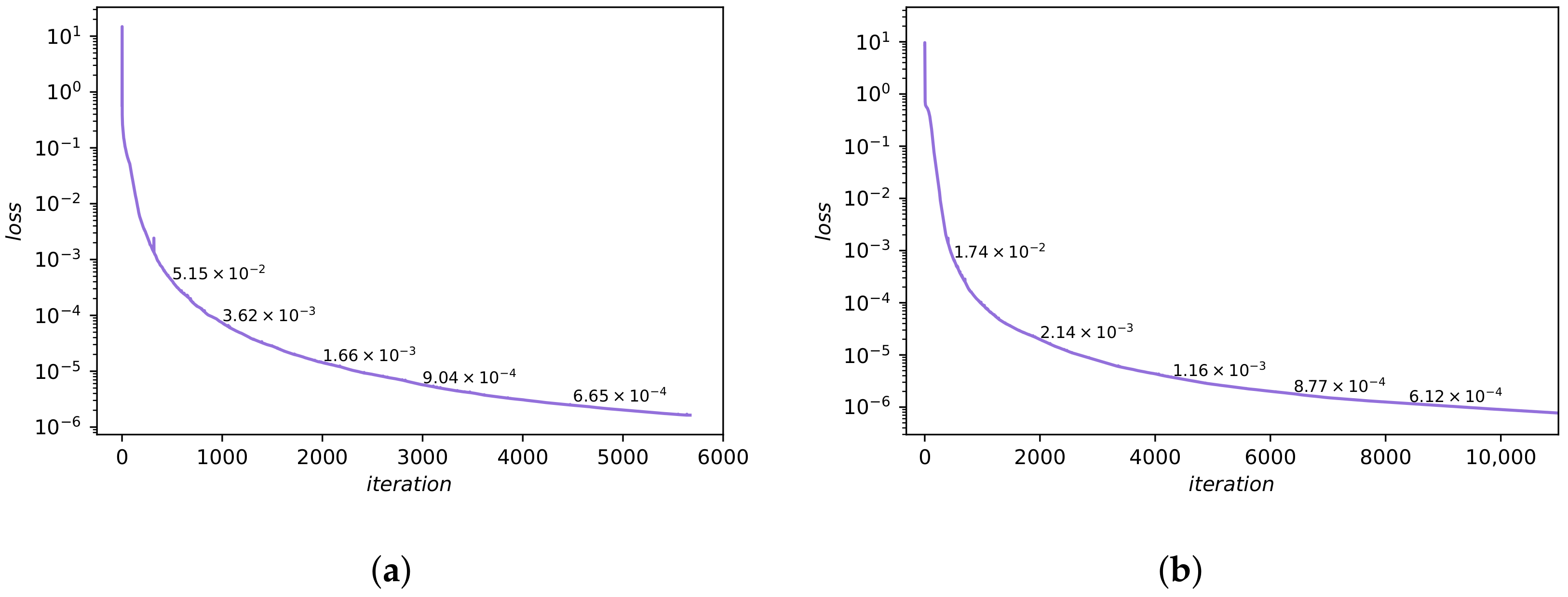
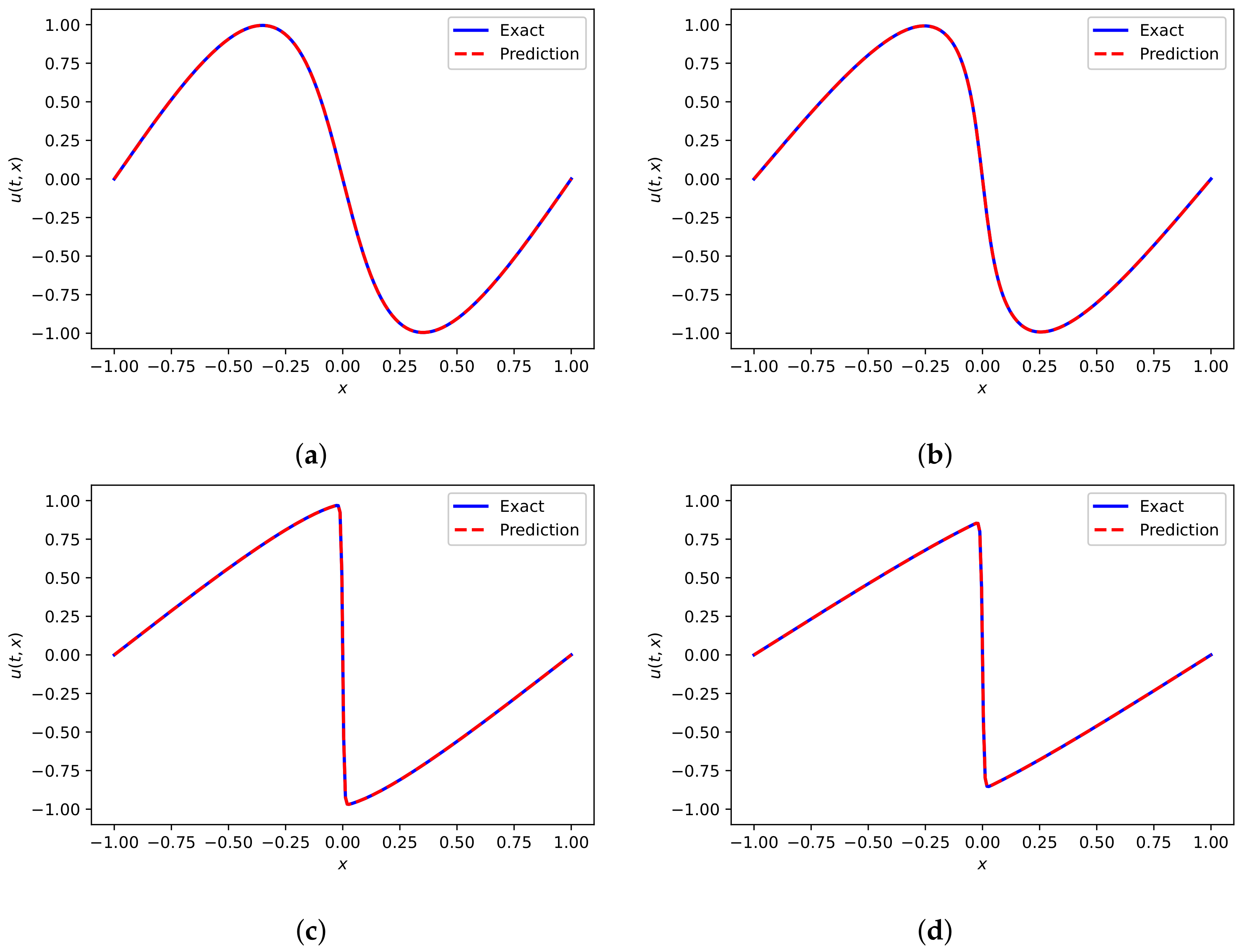
The training set contains collocaction points $N_f$ = 10,000, initial/boundary points $N_u = 200$, and inner points $N_{domain} = 100$. Figure 11a shows the predicted DWNN solution, while the exact solution is recorded in article [54]. Compared with the analytical results, we see that there is no difference between the predicted DWNN solution and the exact solution. Figure 11b shows the change processes of objective functions over the number of iterations under different number of wavelets, from which we find that using four wavelets has the fastest convergence rate but using five works best. In order to display the change process of test error simultaneously, Figure 12a draws the loss curve when the number of wavelets is five separately, and marks the test errors (black text) under different iterations. From this we see that as the number of iterations increases, the loss and test error both decrease. The relative $L^2$ error measured in the end is $2.76 \times {10}^{-4}$. Moreover, a detailed comparison between the predicted solution and analytical result at unequal temporal snapshots $t = (0.15,0.25,0.55,0.75)$ is presented in Figure 13. It is seen that the predicted DWNN solution is indistinguishable from the analytical solution.

To further prove the effectiveness of the proposed method, we carry out the following experimental study to quantify its accuracy.

Table 5. The $L^2$ errors and $L^{\infty }$ errors for 1D Burgers.

${\mathit{L}}^2$ Error		VMWs	$\mathit{l} = 2$	$\mathit{l} = 4$	$\mathit{l} = 6$	$\mathit{l} = 8$
		2	$2.46 \times {10}^{-2}$	$1.02 \times {10}^{-3}$	$4.85 \times {10}^{-4}$	$4.91 \times {10}^{-4}$
		3	$6.41 \times {10}^{-3}$	$1.10 \times {10}^{-3}$	$4.26 \times {10}^{-4}$	$3.70 \times {10}^{-4}$
	DWNN with Equation (39)	4	$1.06 \times {10}^{-2}$	$4.23 \times {10}^{-4}$	$7.35 \times {10}^{-4}$	$3.44 \times {10}^{-4}$
		5	$4.43 \times {10}^{-3}$	$3.39 \times {10}^{-4}$	$3.11 \times {10}^{-4}$	$2.76 \times {10}^{-4}$
		6	$9.71 \times {10}^{-3}$	$6.32 \times {10}^{-4}$	$5.21 \times {10}^{-4}$	$5.70 \times {10}^{-4}$
		7	$1.44 \times {10}^{-2}$	$1.09 \times {10}^{-3}$	$9.07 \times {10}^{-4}$	$1.08 \times {10}^{-3}$
		2	$2.73 \times {10}^{-1}$	$9.71 \times {10}^{-3}$	$4.89 \times {10}^{-3}$	$1.46 \times {10}^{-3}$
		3	$7.30 \times {10}^{-2}$	$1.21 \times {10}^{-2}$	$8.60 \times {10}^{-3}$	$4.12 \times {10}^{-3}$
	WTNN	4	$7.23 \times {10}^{-2}$	$1.02 \times {10}^{-2}$	$2.71 \times {10}^{-3}$	$1.34 \times {10}^{-3}$
		5	$4.86 \times {10}^{-2}$	$1.93 \times {10}^{-3}$	$2.47 \times {10}^{-3}$	$4.30 \times {10}^{-4}$
		6	$9.95 \times {10}^{-2}$	$8.73 \times {10}^{-3}$	$9.67 \times {10}^{-3}$	$4.03 \times {10}^{-3}$
		7	$8.08 \times {10}^{-2}$	$4.37 \times {10}^{-3}$	$3.06 \times {10}^{-3}$	$3.50 \times {10}^{-3}$
	PINN	-	$1.76 \times {10}^{-1}$	$1.02 \times {10}^{-2}$	$5.60 \times {10}^{-3}$	$4.22 \times {10}^{-3}$
${\mathit{L}}^{\infty }$ Error
		2	$2.48 \times {10}^{-1}$	$9.63 \times {10}^{-3}$	$2.74 \times {10}^{-3}$	$4.57 \times {10}^{-3}$
		3	$6.71 \times {10}^{-2}$	$9.18 \times {10}^{-3}$	$2.25 \times {10}^{-3}$	$3.60 \times {10}^{-3}$
	DWNN with Equation (39)	4	$6.74 \times {10}^{-2}$	$5.03 \times {10}^{-3}$	$8.13 \times {10}^{-3}$	$2.49 \times {10}^{-3}$
		5	$3.82 \times {10}^{-2}$	$2.81 \times {10}^{-3}$	$1.55 \times {10}^{-3}$	$1.28 \times {10}^{-3}$
		6	$6.59 \times {10}^{-2}$	$5.78 \times {10}^{-3}$	$3.55 \times {10}^{-3}$	$3.94 \times {10}^{-3}$
		7	$1.06 \times {10}^{-1}$	$1.02 \times {10}^{-2}$	$6.66 \times {10}^{-3}$	$1.07 \times {10}^{-2}$
		2	$1.50$	$8.74 \times {10}^{-2}$	$4.59 \times {10}^{-2}$	$1.28 \times {10}^{-2}$
		3	$8.44 \times {10}^{-1}$	$8.67 \times {10}^{-2}$	$7.81 \times {10}^{-2}$	$4.23 \times {10}^{-2}$
	WTNN	4	$8.41 \times {10}^{-1}$	$7.83 \times {10}^{-2}$	$2.42 \times {10}^{-2}$	$1.27 \times {10}^{-2}$
		5	$5.79 \times {10}^{-1}$	$1.67 \times {10}^{-2}$	$2.31 \times {10}^{-2}$	$4.18 \times {10}^{-3}$
		6	$9.43 \times {10}^{-1}$	$8.59 \times {10}^{-2}$	$9.30 \times {10}^{-2}$	$5.83 \times {10}^{-2}$
		7	$9.24 \times {10}^{-1}$	$3.65 \times {10}^{-2}$	$2.73 \times {10}^{-2}$	$3.97 \times {10}^{-2}$
	PINN	-	$1.58$	$9.66 \times {10}^{-2}$	$5.19 \times {10}^{-2}$	$3.79 \times {10}^{-2}$

summarizes the $L^{\infty }$ errors and $L^2$ errors from three perspectives. First, we show the performance of DWNN model whose cost function contains three terms according to Equation (41). Second, we present the results of DWNN model, which only contains wavelets, and do not add $MS{E}_{domain}$ (we briefly named it WTNN). Lastly, we give the results of other state-of-the-art methods such as PINN. The prediction errors are listed with regard to different number of VMWs and different number of hidden layers, while keeping 20 hidden neurons fixed in each hidden layer. It is clearly seen that considering the residual of a handful of observations into cost function not only achieves the most accuracy but also gives a relatively stable approximation for the solution. Moreover, the DWNN model can achieve high predictive accuracy with fewer hidden layers, which undoubtedly reduces the computational cost. Therefore, the third term of the cost function degenerates when solving the continuous problem, but it is really effective when solving the shock wave problem.

3.1.5. Allen-Cahn Equation

We consider the Allen-Cahn quation with periodic boundary conditions in this subsection. Allen and Cahn jointly introduced this equation to describe the antiphase boundary motion in crystals in 1979 [55]. The Allen–Cahn equation is important to describe fluid dynamics and reaction-diffusion problems in material science. Moreover, the Allen-Cahn equation is generally applied to deal with various problems such as image analysis [56,57], mean curvature flow rate [58], crystal growth [59], and so on. In one-dimensional space, Allen-Cahn equation reads as

$$\left\{\begin{array}{c}{u}_t = 0.0001u_{xx} - 5u^3 + 5u,x \in [-1,1],t \in [0,1],\hfill \\ u(0,x) = x^{2}cos\left(\pi x\right),\hfill \\ u(t,-1) = u(t,1),\hfill \\ u_x(t,-1) = u_x(t,1).\hfill \end{array}\right.$$

(45)

We use the DWNN model which employs five wavelets in wavelet expansion layer and five hidden layers in fully connected part to solve this problem. Each hidden layer contains 60 neurons and a Gaussian error function. The $f(t,x)$ is obtained from Equation (45)

$$f: = u_t - 0.0001u_{xx} + 5u^3 - 5u.$$

(46)

An interesting feature of this equation is the phenomenon of metastable state. The areas of solution close to $\pm 1$ are flat, and the interface between these areas remain unchanged for a long period of time until a sudden change occurs. Therefore, we use the advantage of inner points to rectify the model and randomly choose a few inner points to better deal with the discontinuity of the Allen-Cahn equation. The loss function $J\left(\theta \right)$ is written as

$$MSE = MS{E}_f + MS{E}_0 + MS{E}_b + MS{E}_{domain},$$

(47)

where

$$MS{E}_f = \frac{1}{N_f}\sum _{i=1}^{N_f}{\left|f(t_f^i,x_f^i)\right|}^2,$$

(48)

$$MS{E}_0 = \frac{1}{N_0}\sum _{i=1}^{N_0}{|u(0,x_0^i) - u_0^i|}^2,$$

(49)

$$MS{E}_b = \frac{1}{N_b}\sum _{i=1}^{N_b}\left({|u(t_b^i,-1) - u(t_b^i,1)|}^2 + {|u_x(t_b^i,-1) - u_x(t_b^i,1)|}^2\right),$$

(50)

$$MS{E}_{domain} = \frac{1}{N_{domain}}\sum _{i=1}^{N_{domain}}{|u(t_{domain}^i,x_{domain}^i) - u^i|}^2.$$

(51)

Here, ${\{t_f^i,x_f^i\}}_{i=1}^{N_f}$ specifies the unsupervised collocation points on $f(t,x)$, ${\{x_0^i,u_0^i\}}_{i=1}^{N_0}$ denotes the initial data, ${\left\{t_b^i\right\}}_{i=1}^{N_b}$ denotes the boundary data and ${\{t_{domain}^i,x_{domain}^i\}}_{i=1}^{N_{domain}}$ corresponds to internal sample points in the domain.

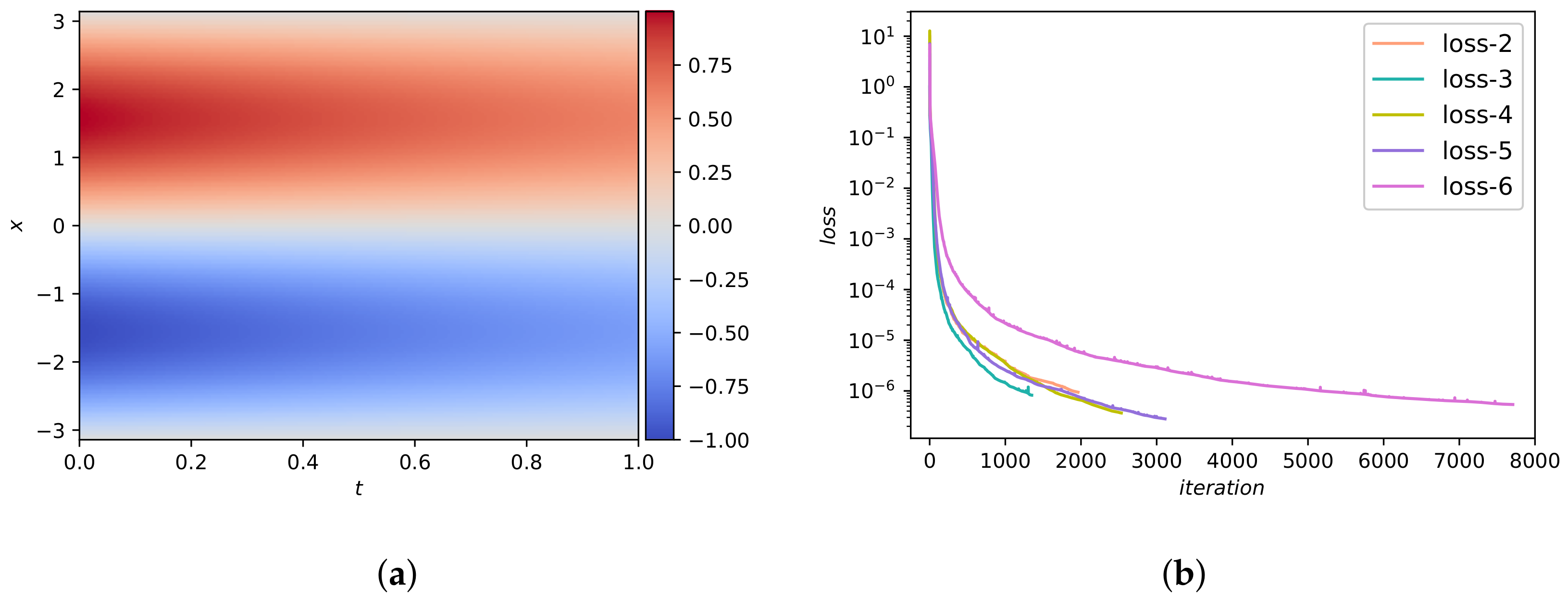
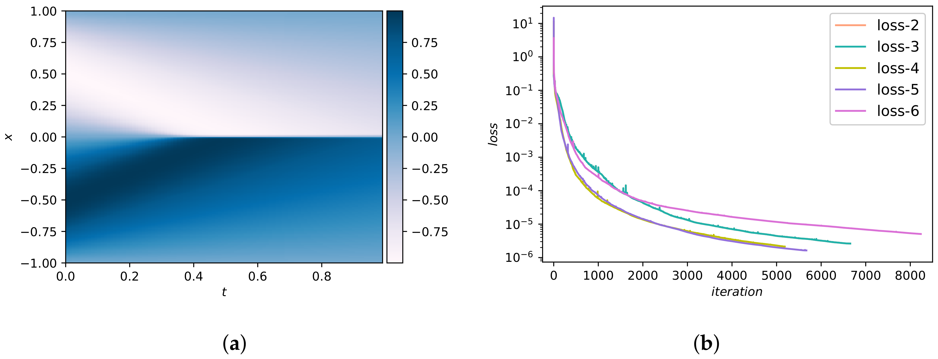
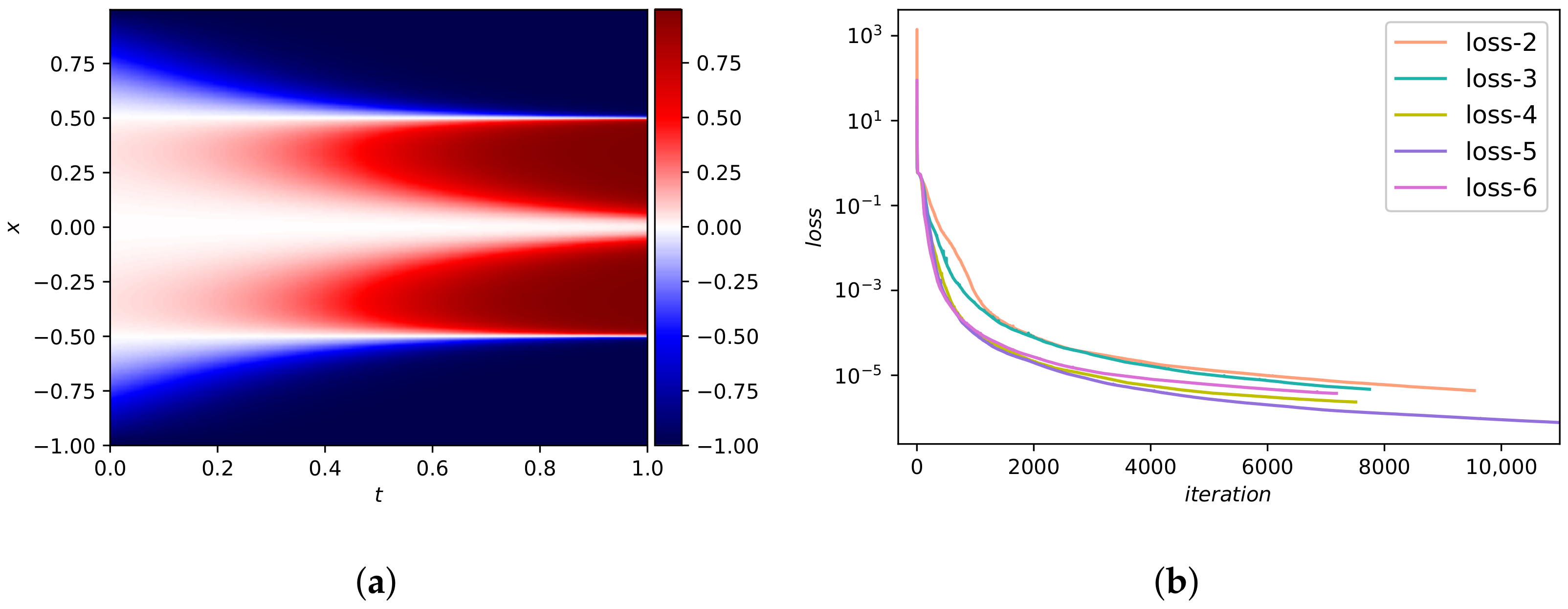
We select 200 inner points in addition to 100 initial/boundary points and 10,000 collocation points to form the training set. The dataset we used was reported in a previous work [24]. They used convolutional spectral methods to simulate an Allen-Cahn equation. Concretely, Equation (45) has integrated from the initial state to the final time using the Chebfun package [42]. Figure 14a shows the predicted value $u(t,x)$ obtained from DWNN model. The predicted value and analytical value are basically the same. The comparison of loss functions for the DWNN model is pictured in Figure 14b. From Figure 14b, we see that the loss function drops quickly when we use five wavelets. Figure 12b shows the loss curve and test errors (black text) using five wavelets. From Figure 12b, we observe that both loss and test errors decrease as the number of iterations increases, as we expected. The error in relative $L^2$-norm is measured at $5.31 \times {10}^{-4}$. In particular, this prediction error is almost three orders of magnitude smaller than the method offered by PINN using continuous time model [24].

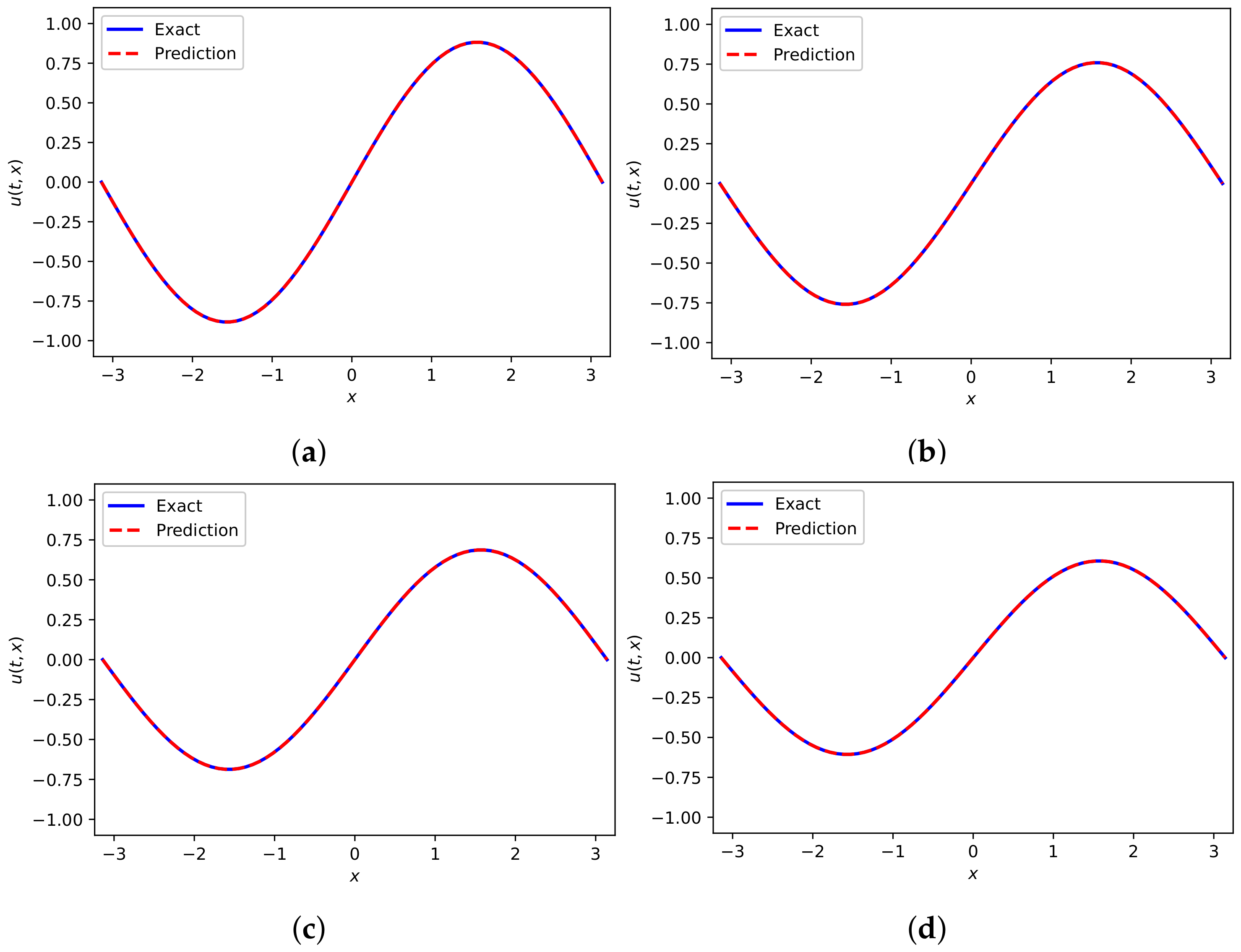
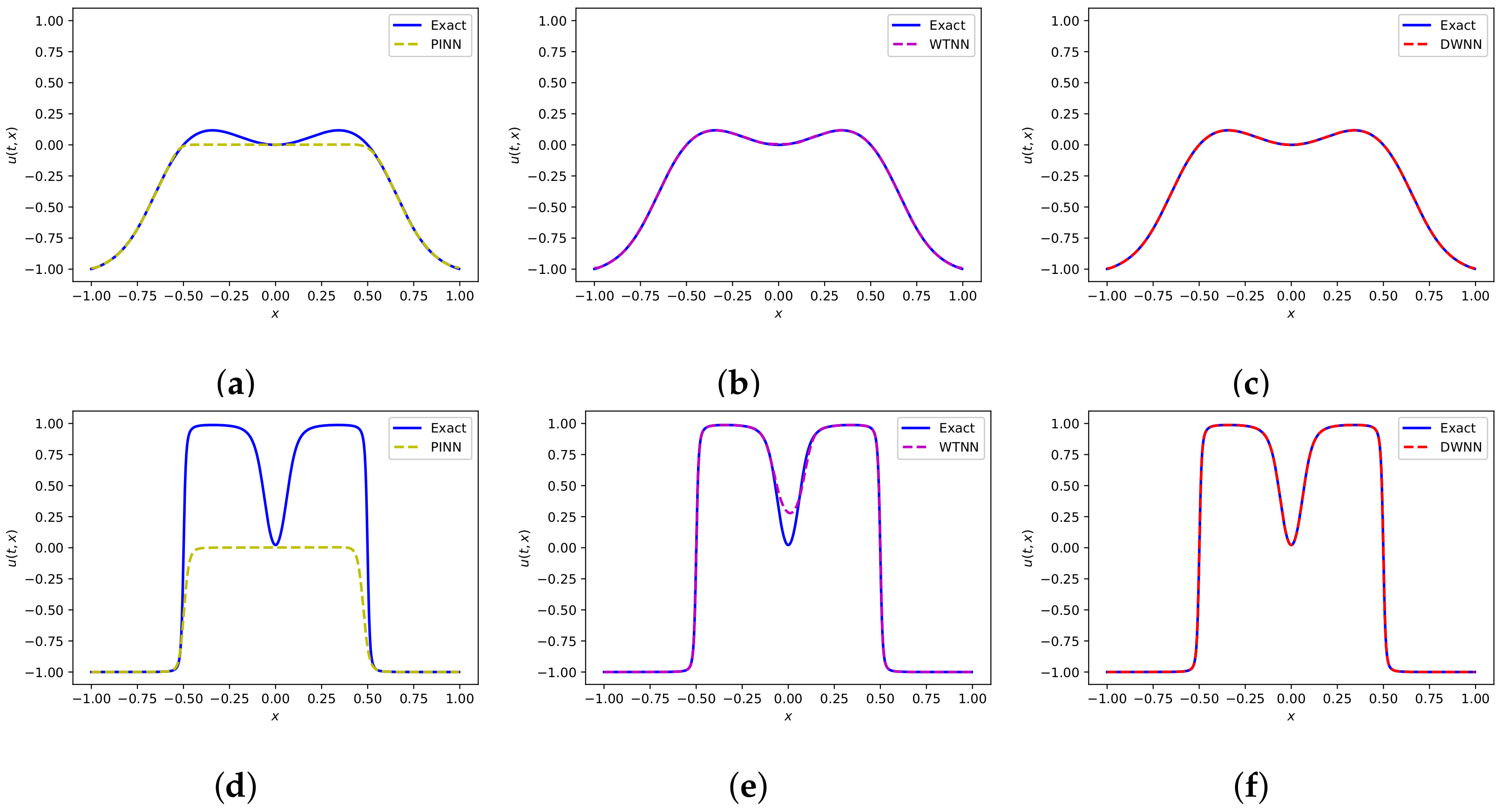
Figure 15 presents the predicted solution based on three methods. Figure 15a,d present the PINN solution at $t = 0.15$ and $t = 0.95$, severally. It is obvious that the PINN solution is not so consistent with the exact solution. Correspondingly, Figure 15b,e display the neural network model which only contains wavelet transform at $t = 0.15$ and $t = 0.95$. It is seen that the predicted solution is better than PINN, but there still exists gaps in some point locations. Figure 15c,f show the DWNN solution at the same time points. We see that the predicted DWNN solution is in perfect agreement with the exact solution. As we can find from Figure 15, the experimental results of DWNN model are closer to the analytical results. Furthermore, we report the $L^{\infty }$ errors and $L^2$ errors based on PINN, WTNN and DWNN for different number of VMWs, and different number of hidden layers. Here, the number of neurons are fixed to 60 in each hidden layer. The results are listed in

Table 6. The $L^2$ errors and $L^{\infty }$ errors for 1D Allen-Cahn.

${\mathit{L}}^2$ Error		VMWs	$\mathit{l} = 3$	$\mathit{l} = 5$	$\mathit{l} = 7$	$\mathit{l} = 9$
		2	$1.42 \times {10}^{-3}$	$1.24 \times {10}^{-3}$	$7.25 \times {10}^{-4}$	$1.04 \times {10}^{-3}$
		3	$1.87 \times {10}^{-3}$	$1.45 \times {10}^{-3}$	$1.08 \times {10}^{-3}$	$1.17 \times {10}^{-2}$
	DWNN with Equation (45)	4	$1.11 \times {10}^{-3}$	$6.81 \times {10}^{-4}$	$4.72 \times {10}^{-4}$	$6.22 \times {10}^{-4}$
		5	$1.07 \times {10}^{-3}$	$5.31 \times {10}^{-4}$	$6.58 \times {10}^{-4}$	$8.46 \times {10}^{-4}$
		6	$1.05 \times {10}^{-3}$	$8.52 \times {10}^{-4}$	$7.22 \times {10}^{-4}$	$6.18 \times {10}^{-4}$
		7	$1.00 \times {10}^{-3}$	$7.01 \times {10}^{-4}$	$6.17 \times {10}^{-4}$	$8.94 \times {10}^{-4}$
		2	$1.47 \times {10}^{-1}$	$9.64 \times {10}^{-2}$	$5.63 \times {10}^{-2}$	$7.87 \times {10}^{-2}$
		3	$1.20 \times {10}^{-1}$	$7.04 \times {10}^{-2}$	$7.09 \times {10}^{-2}$	$7.17 \times {10}^{-2}$
	WTNN	4	$7.38 \times {10}^{-2}$	$6.35 \times {10}^{-2}$	$6.81 \times {10}^{-2}$	$4.94 \times {10}^{-2}$
		5	$6.05 \times {10}^{-2}$	$3.83 \times {10}^{-2}$	$5.10 \times {10}^{-2}$	$4.23 \times {10}^{-2}$
		6	$5.61 \times {10}^{-2}$	$4.34 \times {10}^{-2}$	$1.95 \times {10}^{-2}$	$3.96 \times {10}^{-2}$
		7	$6.55 \times {10}^{-2}$	$4.76 \times {10}^{-2}$	$5.07 \times {10}^{-2}$	$4.76 \times {10}^{-2}$
	PINN	-	$1.40 \times {10}^{-1}$	$5.24 \times {10}^{-1}$	$5.34 \times {10}^{-1}$	$9.55 \times {10}^{-1}$
${\mathit{L}}^{\infty }$ Error
		2	$3.88 \times {10}^{-2}$	$3.77 \times {10}^{-2}$	$2.32 \times {10}^{-2}$	$3.46 \times {10}^{-2}$
		3	$4.67 \times {10}^{-2}$	$4.52 \times {10}^{-2}$	$3.44 \times {10}^{-2}$	$3.63 \times {10}^{-2}$
	DWNN with Equation (45)	4	$2.70 \times {10}^{-2}$	$2.80 \times {10}^{-2}$	$2.08 \times {10}^{-2}$	$2.50 \times {10}^{-2}$
		5	$3.50 \times {10}^{-2}$	$2.21 \times {10}^{-2}$	$2.77 \times {10}^{-2}$	$2.39 \times {10}^{-3}$
		6	$3.18 \times {10}^{-2}$	$3.04 \times {10}^{-2}$	$2.82 \times {10}^{-2}$	$2.44 \times {10}^{-2}$
		7	$2.48 \times {10}^{-2}$	$2.49 \times {10}^{-2}$	$2.48 \times {10}^{-2}$	$2.57 \times {10}^{-2}$
		2	$8.70 \times {10}^{-1}$	$7.52 \times {10}^{-1}$	$5.41 \times {10}^{-1}$	$6.77 \times {10}^{-1}$
		3	$7.84 \times {10}^{-1}$	$6.25 \times {10}^{-1}$	$6.30 \times {10}^{-1}$	$6.63 \times {10}^{-1}$
	WTNN	4	$6.43 \times {10}^{-1}$	$5.87 \times {10}^{-1}$	$6.16 \times {10}^{-1}$	$4.90 \times {10}^{-1}$
		5	$5.37 \times {10}^{-1}$	$3.97 \times {10}^{-1}$	$4.95 \times {10}^{-1}$	$4.25 \times {10}^{-1}$
		6	$5.27 \times {10}^{-1}$	$4.44 \times {10}^{-1}$	$2.30 \times {10}^{-1}$	$4.11 \times {10}^{-1}$
		7	$5.91 \times {10}^{-1}$	$4.51 \times {10}^{-1}$	$4.48 \times {10}^{-1}$	$4.57 \times {10}^{-1}$
	PINN	-	$8.49 \times {10}^{-1}$	$1.51$	$1.55$	$1.00$

. Apparently, when dealing with interface problems, adding the residual term of observation points can improve the predictive accuracy significantly.

3.2. Two-Dimensional Equations

In this subsecion, three two-dimensional equations are presented so as to further demonstrate the perfomance of the proposed method.

3.2.1. Burgers Equation

In two-dimensional space, the form of Burgers equation [54] is

$$u_t = -u{u}_x - u{u}_y + 0.1(u_{x}x + u_{y}y),(x,y) \in [0,1] \times [0,1],t \in [0,3],$$

(52)

where the initial/boundary conditions are extracted from analytical solution given by

$$u(t,x,y) = 1/(1 + e^{(x+y-t)/0.2}).$$

(53)

In this part, we exploit the deep wavelet neural network which consists of wavelet expansional layer with six wavelets and a fully connected neural network with seven hidden layers. Each hidden layer contains 20 hidden neurons. The activation function remains the same. The $f(t,x,y)$ is obtained from Equation (52)

$$f: = u_t + u{u}_x + u{u}_y - 0.1(u_{x}x + u_{y}y).$$

(54)

The target parameters of neural network are trained by minimizing the loss function $J\left(\theta \right)$

$$J\left(\theta \right) = MS{E}_f + MS{E}_u,$$

(55)

where

$$MS{E}_f = \frac{1}{N_f}\sum _{i=1}^{N_f}{\left|f(t_f^i,x_f^i,y_f^i)\right|}^2,$$

(56)

$$MS{E}_u = \frac{1}{N_u}\sum _{i=1}^{N_u}{|u(t_u^i,x_u^i,y_u^i) - u^i|}^2.$$

(57)

The collocation points are 20,000 whereas the initial/boundary points are 150. The predicted DWNN solution at time instant $t = 1$ is presented in Figure 16b. To see it more precisely, we show the analytical solution at time instant $t = 1$ in Figure 16a. It is hard to see any difference between them. The relative $L^2$ error calculated is $3.25 \times {10}^{-4}$. Figure 16c depicts the error visually at $t = 1$. As we can see, the error is so small in most areas except for a few points. The progresses of the loss functions versus iterations are plotted in Figure 16d. The objective function reaches the minimum value in the case of six wavelets. We give a systematic research on the $L^{\infty }$ errors and $L^2$ errors with regard to different number of VMWs and different number of hidden layers when the neurons are set to 20 per hidden layer. The results are displayed in

Table 7. The $L^2$ errors and $L^{\infty }$ errors for 2D Burgers.

${\mathit{L}}^2$ Error		VMWs	$\mathit{l} = 3$	$\mathit{l} = 5$	$\mathit{l} = 7$	$\mathit{l} = 9$
		2	$2.26 \times {10}^{-3}$	$1.47 \times {10}^{-3}$	$1.75 \times {10}^{-3}$	$1.19 \times {10}^{-3}$
		3	$1.78 \times {10}^{-3}$	$1.94 \times {10}^{-3}$	$1.55 \times {10}^{-3}$	$1.25 \times {10}^{-2}$
	DWNN with Equation (52)	4	$9.11 \times {10}^{-4}$	$7.17 \times {10}^{-4}$	$1.13 \times {10}^{-3}$	$1.00 \times {10}^{-3}$
		5	$6.85 \times {10}^{-4}$	$7.14 \times {10}^{-4}$	$4.35 \times {10}^{-4}$	$3.88 \times {10}^{-4}$
		6	$3.57 \times {10}^{-4}$	$5.04 \times {10}^{-4}$	$3.25 \times {10}^{-4}$	$4.75 \times {10}^{-4}$
		7	$1.24 \times {10}^{-3}$	$6.70 \times {10}^{-4}$	$7.49 \times {10}^{-4}$	$6.82 \times {10}^{-4}$
	PINN	-	$1.14 \times {10}^{-3}$	$1.02 \times {10}^{-3}$	$8.89 \times {10}^{-4}$	$5.67 \times {10}^{-4}$
${\mathit{L}}^{\infty }$ Error
		2	$1.66 \times {10}^{-2}$	$1.90 \times {10}^{-2}$	$8.18 \times {10}^{-3}$	$7.73 \times {10}^{-3}$
		3	$8.76 \times {10}^{-3}$	$1.71 \times {10}^{-2}$	$1.18 \times {10}^{-2}$	$9.33 \times {10}^{-2}$
	DWNN with Equation (52)	4	$1.43 \times {10}^{-2}$	$6.87 \times {10}^{-3}$	$9.04 \times {10}^{-3}$	$1.09 \times {10}^{-2}$
		5	$4.02 \times {10}^{-3}$	$8.43 \times {10}^{-3}$	$2.96 \times {10}^{-3}$	$4.81 \times {10}^{-3}$
		6	$3.01 \times {10}^{-3}$	$9.67 \times {10}^{-3}$	$3.59 \times {10}^{-3}$	$4.28 \times {10}^{-3}$
		7	$1.31 \times {10}^{-2}$	$4.39 \times {10}^{-3}$	$9.62 \times {10}^{-3}$	$5.32 \times {10}^{-3}$
	PINN	-	$7.28 \times {10}^{-3}$	$5.55 \times {10}^{-3}$	$4.33 \times {10}^{-3}$	$1.80 \times {10}^{-3}$

. It can be seen from the table that it tends to be stable starting from the use of five wavelets.

3.2.2. Schrödinger Equation

In two-dimensional space, we consider Schrödinger equation with the Dirichlet boundary conditions

$$i{h}_t + h_{xx} + h_{yy} + w(x,y)h = 0,t \in [0,1],(x,y) \in [-5,5] \times [-5,5],$$

(58)

where the potential function $w(x,y) = 3 - 2tan{h}^{2}x - 2tan{h}^{2}y$. The analytical solution for this equation is

$$h(t,x,y) = {\displaystyle \frac{i{e}^{it}}{coshxcoshy}}.$$

(59)

We adopt six wavelets and a followed fully connected neural network with 4 hidden layers. Each hidden layer has 50 hidden neurons. The $f(t,x,y)$ is obtained from the left-hand-side of Equation (58)

$$f := i{h}_t + h_{xx} + h_{yy} + w(x,y)h.$$

(60)

Similar to the previous case in Section 3.1.1, the entire solution $h(t,x,y)$ is rewritten as $h(t,x,y) = \left[u\right(t,x,y),v(t,x,y\left)\right]$, which means the network is also multi-output. The DWNN parameters are obtained by minimizing the mean squared error loss $J\left(\theta \right)$

$$J\left(\theta \right) = MS{E}_f + MS{E}_h,$$

(61)

where

$$MS{E}_f = \frac{1}{N_f}\sum _{i=1}^{N_f}{\left|f(t_f^i,x_f^i,y_f^i)\right|}^2,$$

(62)

$$MS{E}_h = \frac{1}{N_h}\sum _{i=1}^{N_h}{|h(t_h^i,x_h^i,y_h^i) - h^i|}^2.$$

(63)

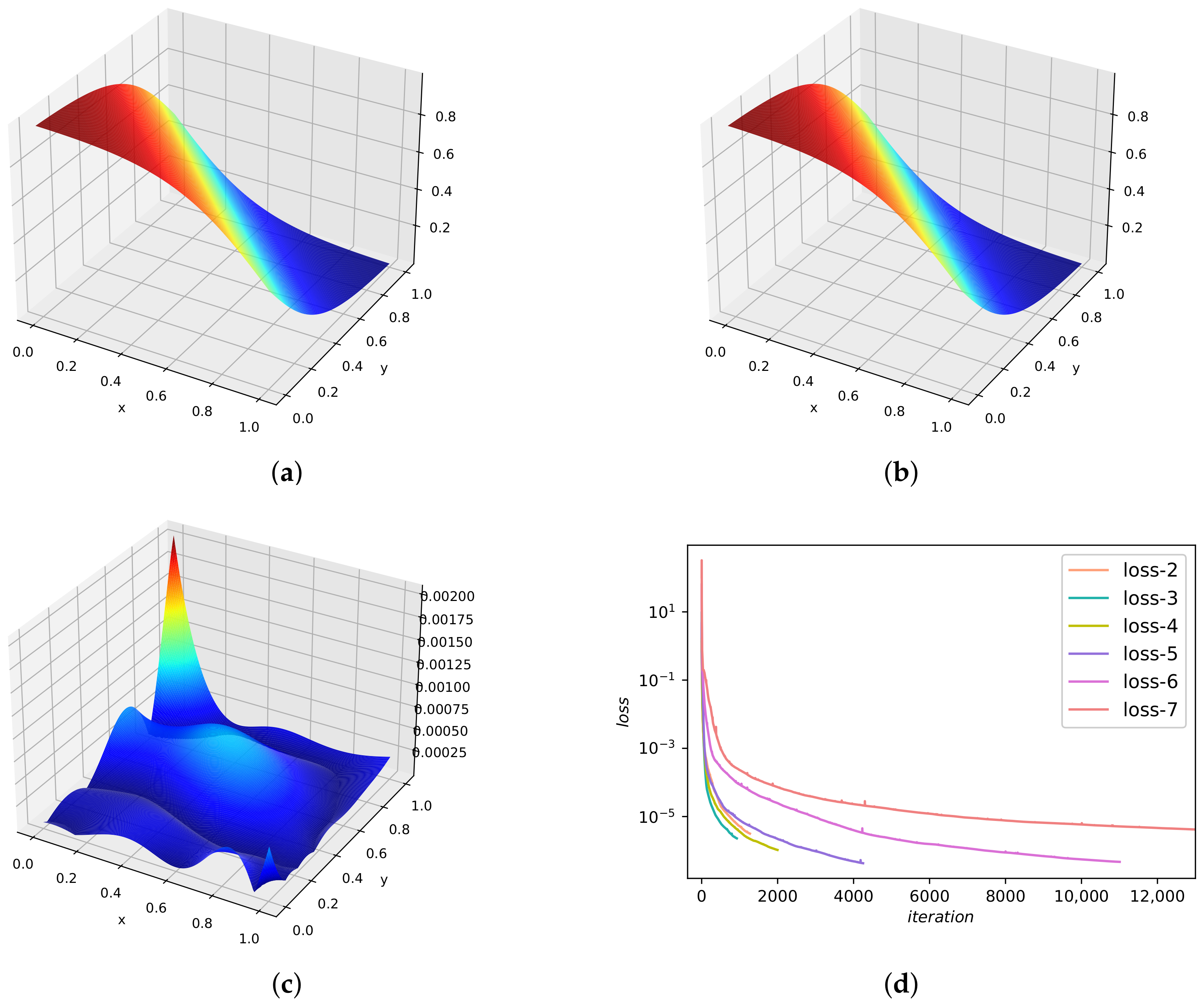
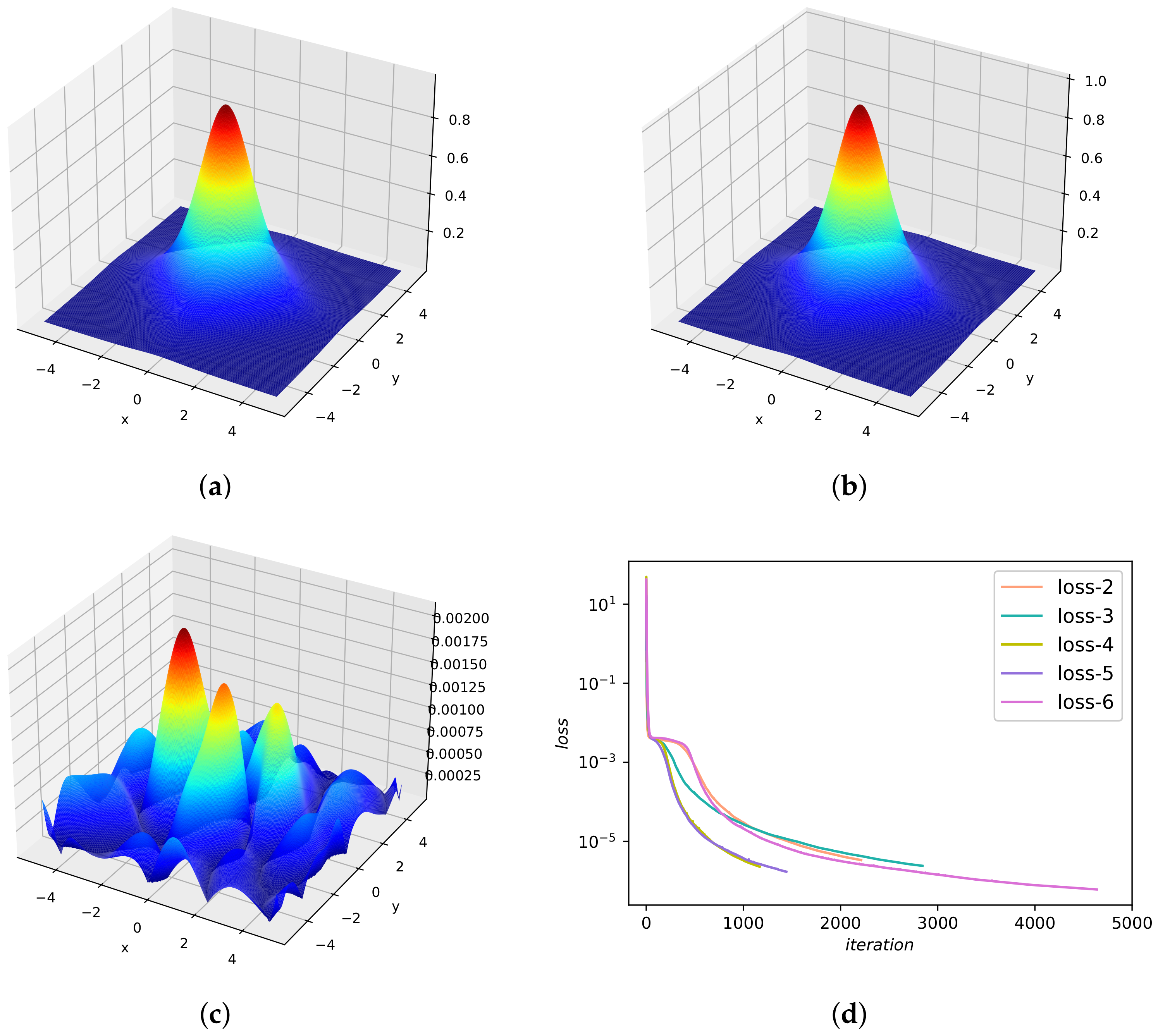
The number of collocation points is 20,000, and the number of training data on the initial/boundary is 150. The entire solution $\left|h\right(t,x,y\left)\right|$ at time instant $t = 0.1$ obtained from analytical solution [39] and DWNN model are shown in Figure 17a,b, respectively. Coming to the comparison of them, we can observe similar results. Figure 17c presents the absolute error for $\left|h\right|$ at $t = 0.1$ and the relative $L^2$ error calculated for this instance is $2.39 \times {10}^{-3}$. It suggests that the simulation result is consistent with the theoretical result. The trends of loss functions versus iterations are presented in Figure 17d, from which we find that the loss function is continuously reduced to the minimum under six wavelets. In

Table 8. The $L^2$ errors and $L^{\infty }$ errors for 2D Schrödinger.

${\mathit{L}}^2$ Error		VMWs	$\mathit{l} = 2$	$\mathit{l} = 4$	$\mathit{l} = 6$	$\mathit{l} = 8$
		2	$1.66 \times {10}^{-2}$	$1.41 \times {10}^{-2}$	$7.64 \times {10}^{-3}$	$6.87 \times {10}^{-3}$
		3	$1.67 \times {10}^{-2}$	$9.80 \times {10}^{-3}$	$8.45 \times {10}^{-3}$	$8.34 \times {10}^{-3}$
	DWNN with Equation (58)	4	$1.50 \times {10}^{-2}$	$9.49 \times {10}^{-3}$	$7.09 \times {10}^{-3}$	$4.69 \times {10}^{-3}$
		5	$1.15 \times {10}^{-2}$	$8.59 \times {10}^{-3}$	$6.05 \times {10}^{-3}$	$8.70 \times {10}^{-3}$
		6	$1.08 \times {10}^{-2}$	$2.39 \times {10}^{-3}$	$6.07 \times {10}^{-3}$	$4.59 \times {10}^{-3}$
	PINN	-	$1.66 \times {10}^{-2}$	$1.57 \times {10}^{-2}$	$7.92 \times {10}^{-3}$	$1.14 \times {10}^{-2}$
${\mathit{L}}^{\infty }$ Error
		2	$2.27 \times {10}^{-2}$	$1.87 \times {10}^{-2}$	$1.02 \times {10}^{-2}$	$8.84 \times {10}^{-3}$
		3	$2.17 \times {10}^{-2}$	$1.11 \times {10}^{-2}$	$1.28 \times {10}^{-2}$	$1.13 \times {10}^{-2}$
	DWNN with Equation (58)	4	$1.67 \times {10}^{-2}$	$1.49 \times {10}^{-3}$	$1.26 \times {10}^{-2}$	$4.72 \times {10}^{-3}$
		5	$1.45 \times {10}^{-2}$	$1.07 \times {10}^{-3}$	$7.33 \times {10}^{-3}$	$9.42 \times {10}^{-3}$
		6	$1.26 \times {10}^{-2}$	$2.32 \times {10}^{-3}$	$7.69 \times {10}^{-3}$	$5.34 \times {10}^{-3}$
	PINN	-	$2.32 \times {10}^{-2}$	$1.05 \times {10}^{-2}$	$1.06 \times {10}^{-2}$	$1.33 \times {10}^{-2}$

, we list the resulting prediction errors in $L^{\infty }$-norm and $L^2$-norm for different number of VMWs and different number of hidden layers. The number of neurons are fixed to 50 in each hidden layer. The results show that as the number of VMWs increases, the predictive accuracy improves in general.

3.2.3. Helmholtz Equation

In two dimensions, we consider the Helmholtz equation with homogeneous Dirichlet boundary conditions

$$\Delta u + k^{2}u = q(x,y),(x,y) \in [-1,1] \times [-1,1],$$

(64)

where the forcing term is given by

$$q(x,y) = 2\pi cos\left(\pi y\right)sin\left(\pi x\right) + 2\pi cos\left(\pi x\right)sin\left(\pi y\right) + (x+y)sin\left(\pi x\right)sin\left(\pi y\right)-2{\pi }^2(x + y)sin\left(\pi x\right)sin\left(\pi y\right).$$

(65)

In this case, we consider $k = 1$ and the corresponding exact solution is $u(x,y) = (x+y)sin\left(\pi x\right)sin\left(\pi y\right)$. Here, five wavelets are used in wavelet expansion layer. There are six following hidden layers and each layer contains 40 neurons. The $f(x,y)$ is obtained from Equation (64)

$$f := \Delta u + k^{2}u - q(x,y).$$

(66)

The optimal parameters are learned by minimizing the loss function $J\left(\theta \right)$

$$J\left(\theta \right) = MS{E}_f + MS{E}_u,$$

(67)

where

$$MS{E}_f = \frac{1}{N_f}\sum _{i=1}^{N_f}{\left|f(x_f^i,y_f^i)\right|}^2,$$

(68)

$$MS{E}_u = \frac{1}{N_u}\sum _{i=1}^{N_u}{|u(x_u^i,y_u^i) - u^i|}^2.$$

(69)

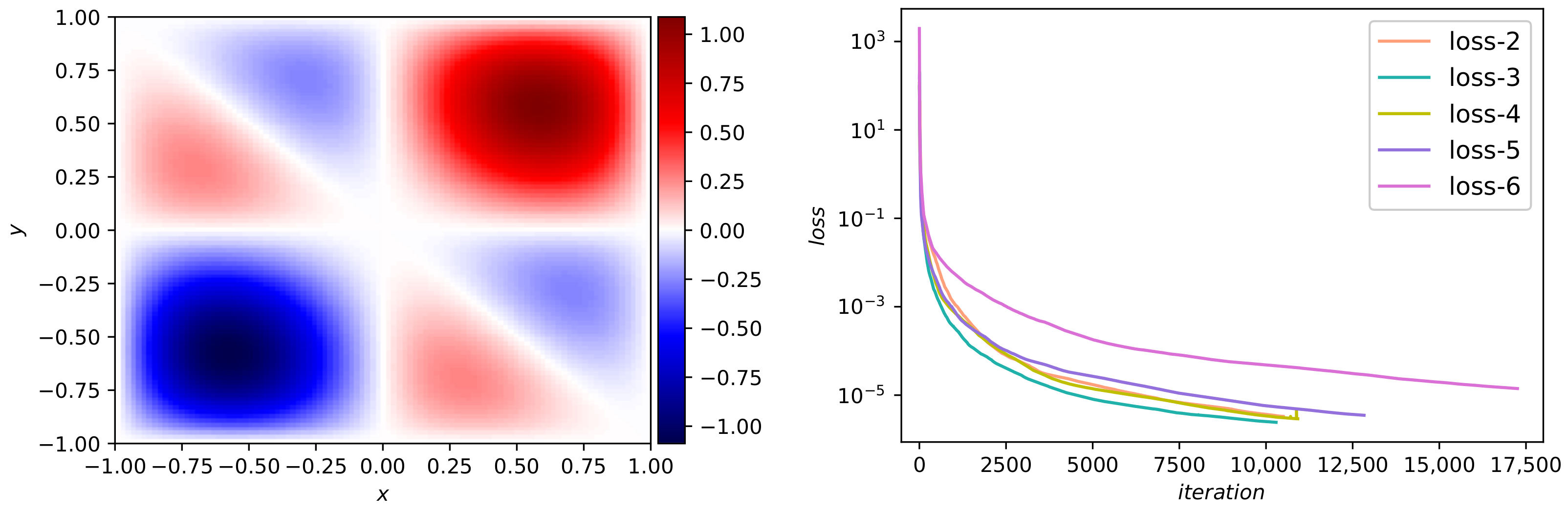
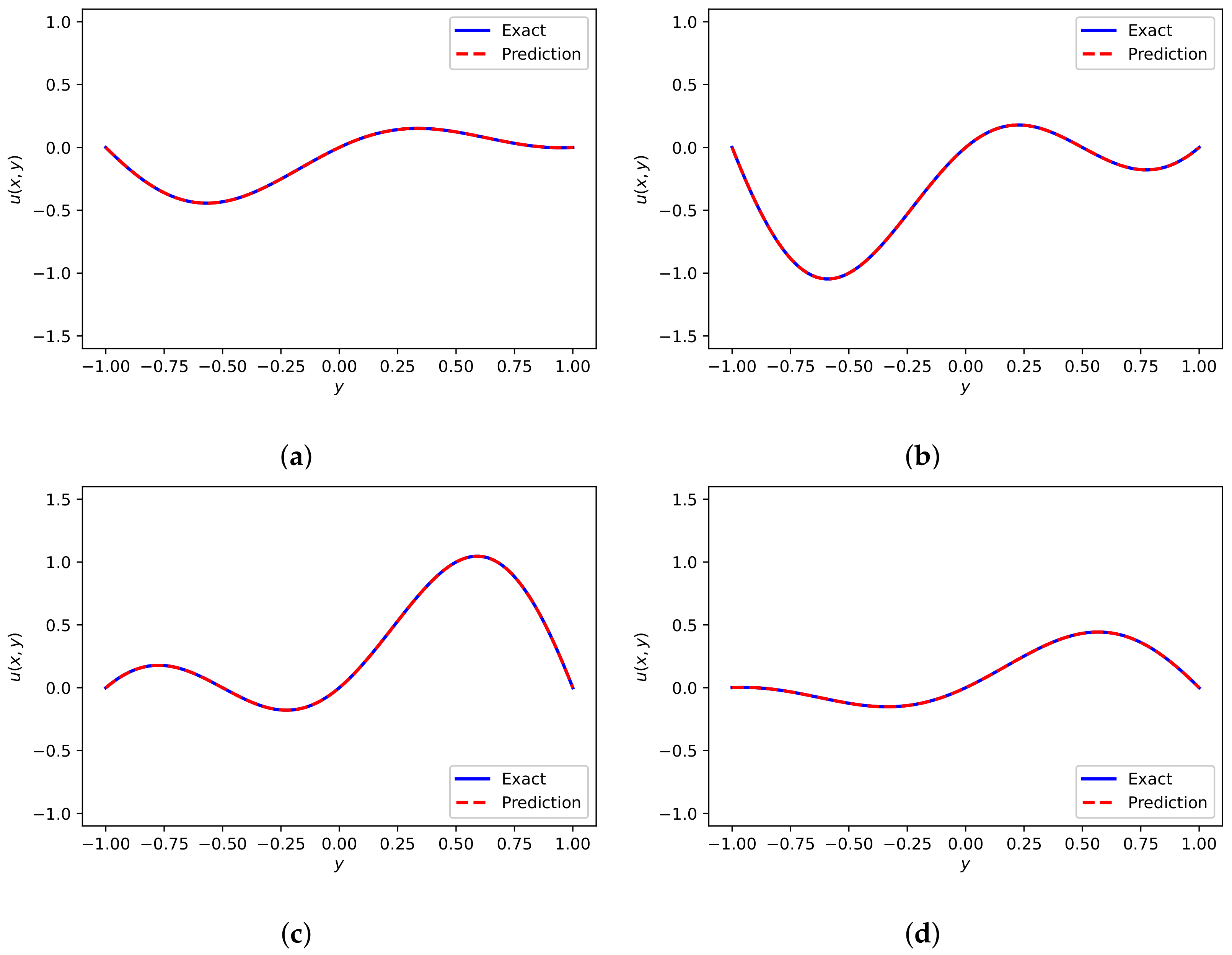
The training data, $N_u$, are 400, whereas the residual training data, $N_f$, are 16,000. Figure 18a presents the contour plot of predicted result of Helmholtz equation. This prediction seems to be identical to the theoretical solution [50]. Figure 18b presents the change trends of loss functions versus iterations, from which we see the best convergence of five wavelets. The relative $L^2$ error measured in the end is $2.86 \times {10}^{-4}$. We plot the comparison of DWNN results and analytical results at $x = (-0.9,-0.5,0.5,0.9)$ as shown in Figure 19. In these figures we find that the simulation solution is in consistent with the law of physics and the analytical solution. A detailed experimental study to quantify the impact of unequal number of VMWs and different layers of network is presented in

Table 9. The $L^2$ errors and $L^{\infty }$ errors for 2D Helmholtz.

${\mathit{L}}^2$ Error		VMWs	$\mathit{l} = 2$	$\mathit{l} = 4$	$\mathit{l} = 6$	$\mathit{l} = 8$
		2	$5.57 \times {10}^{-4}$	$8.33 \times {10}^{-4}$	$1.07 \times {10}^{-3}$	$2.88 \times {10}^{-3}$
		3	$3.97 \times {10}^{-4}$	$4.45 \times {10}^{-4}$	$9.92 \times {10}^{-4}$	$6.99 \times {10}^{-4}$
	DWNN with Equation (64)	4	$5.09 \times {10}^{-4}$	$8.84 \times {10}^{-4}$	$4.01 \times {10}^{-4}$	$9.17 \times {10}^{-4}$
		5	$5.76 \times {10}^{-4}$	$5.81 \times {10}^{-4}$	$2.86 \times {10}^{-4}$	$6.51 \times {10}^{-4}$
		6	$1.49 \times {10}^{-3}$	$1.08 \times {10}^{-3}$	$7.39 \times {10}^{-4}$	$5.17 \times {10}^{-4}$
		7	$2.65 \times {10}^{-3}$	$2.46 \times {10}^{-3}$	$1.75 \times {10}^{-3}$	$1.15 \times {10}^{-3}$
	PINN	-	$7.42 \times {10}^{-3}$	$1.40 \times {10}^{-2}$	$2.20 \times {10}^{-2}$	$5.26 \times {10}^{-2}$
${\mathit{L}}^{\infty }$ Error
		2	$1.88 \times {10}^{-3}$	$2.64 \times {10}^{-3}$	$2.73 \times {10}^{-3}$	$5.99 \times {10}^{-3}$
		3	$1.70 \times {10}^{-3}$	$1.10 \times {10}^{-3}$	$2.44 \times {10}^{-3}$	$1.56 \times {10}^{-3}$
	DWNN with Equation (64)	4	$1.84 \times {10}^{-3}$	$2.61 \times {10}^{-3}$	$1.32 \times {10}^{-3}$	$2.31 \times {10}^{-3}$
		5	$1.44 \times {10}^{-3}$	$1.50 \times {10}^{-3}$	$8.19 \times {10}^{-4}$	$1.99 \times {10}^{-3}$
		6	$3.46 \times {10}^{-3}$	$3.01 \times {10}^{-3}$	$2.10 \times {10}^{-3}$	$1.39 \times {10}^{-3}$
		7	$9.95 \times {10}^{-3}$	$6.49 \times {10}^{-3}$	$4.85 \times {10}^{-3}$	$3.66 \times {10}^{-3}$
	PINN	-	$1.20 \times {10}^{-2}$	$3.41 \times {10}^{-2}$	$3.39 \times {10}^{-2}$	$1.11 \times {10}^{-1}$

. By fixing the number of neurons in each hidden layer to 40, we vary the number of wavelets and hidden layers, and monitor the resulting $L^{\infty }$ errors and $L^2$ errors for the predicted solution. The general trend shows that the predictive accuracy is improved obviously by the addition of wavelet extension layer.

3.2.4. Flow in a Lid-Driven Cavity

In this subsection, we consider the steady-state flow in a two-dimensional lid-driven cavity, which is a typical incompressible viscous fluid model in computational fluid mechanics. The system is governed by the incompressible Navier-Stokes equations, which can be written as [60]

$$\left\{\begin{array}{c}\mathit{u} · \nabla \mathit{u} + \nabla p - \frac{1}{Re}\Delta \mathit{u} = 0,\mathrm{in}\mathrm{\Omega },\hfill \\ \nabla · \mathit{u} = 0,\mathrm{in}\mathrm{\Omega },\hfill \\ \mathit{u}(x,y) = (1,0),\mathrm{on}{\mathrm{\Gamma }}_1,\hfill \\ \mathit{u}(x,y) = (0,0),\mathrm{on}{\mathrm{\Gamma }}_0.\hfill \end{array}\right.$$

(70)

Here, $\mathit{u} = (u,v)$ is the velocity field and p is the pressure field. $u(x,y)$ represents the x-component of the velocity vector field and $v(x,y)$ represents the y-component. The computational domain $\mathrm{\Omega } = (0,1) \times (0,1)$. ${\mathrm{\Gamma }}_1$ denotes the top boundary of the 2-D square cavity and ${\mathrm{\Gamma }}_0$ denotes the other three sides. Reynolds number (Re) is a non-dimensional number used to characterize fluid flow and we consider $Re = 100$. We make an assumption according to Wang et al. [60] that

$$u = \frac{\partial \psi }{\partial y},v = -\frac{\partial \psi }{\partial x}$$

(71)

Under this assumption, the incompressibility constraint is automatically satisfied. The $f(x,y)$ is obtained from Equation (70)

$$\begin{array}{cc}\hfill & f_1 := u\frac{\partial u}{\partial x} + v\frac{\partial u}{\partial y} + \frac{\partial p}{\partial x} - \frac{1}{100}(\frac{{\partial }^{2}u}{\partial x^2} + \frac{{\partial }^{2}u}{\partial y^2}),\hfill \end{array}$$

(72a)

$$\begin{array}{cc}\hfill & f_2 := u\frac{\partial v}{\partial x} + v\frac{\partial v}{\partial y} + \frac{\partial p}{\partial y} - \frac{1}{100}(\frac{{\partial }^{2}v}{\partial x^2} + \frac{{\partial }^{2}v}{\partial y^2}).\hfill \end{array}$$

(72b)

where $(u,v) = (\partial \psi /\partial y,v = -\partial \psi /\partial x)$. Therefore, the neural network is multi-output because two units are needed to represent $\psi$ and p, respectively. The cost function $J\left(\theta \right)$ is given by

$$J\left(\theta \right) = MS{E}_f + MS{E}_{u_b} + MS{E}_{v_b},$$

(73)

where

$$MS{E}_f = \frac{1}{N_f}\sum _{i=1}^{N_f}{\left|f_1(x_f^i,y_f^i)\right|}^2+\frac{1}{N_f}\sum _{i=1}^{N_f}{\left|f_2(x_f^i,y_f^i)\right|}^2,$$

(74)

$$MS{E}_{u_b} = \frac{1}{N_{u_b}}\sum _{i=1}^{N_{u_b}}({|u(x_{u_b}^i,y_{u_b}^i) - u^i|}^2,$$

(75)

$$MS{E}_{v_b} = \frac{1}{N_{v_b}}\sum _{i=1}^{N_{v_b}}{|v(x_{v_b}^i,y_{v_b}^i) - v^i|}^2.$$

(76)

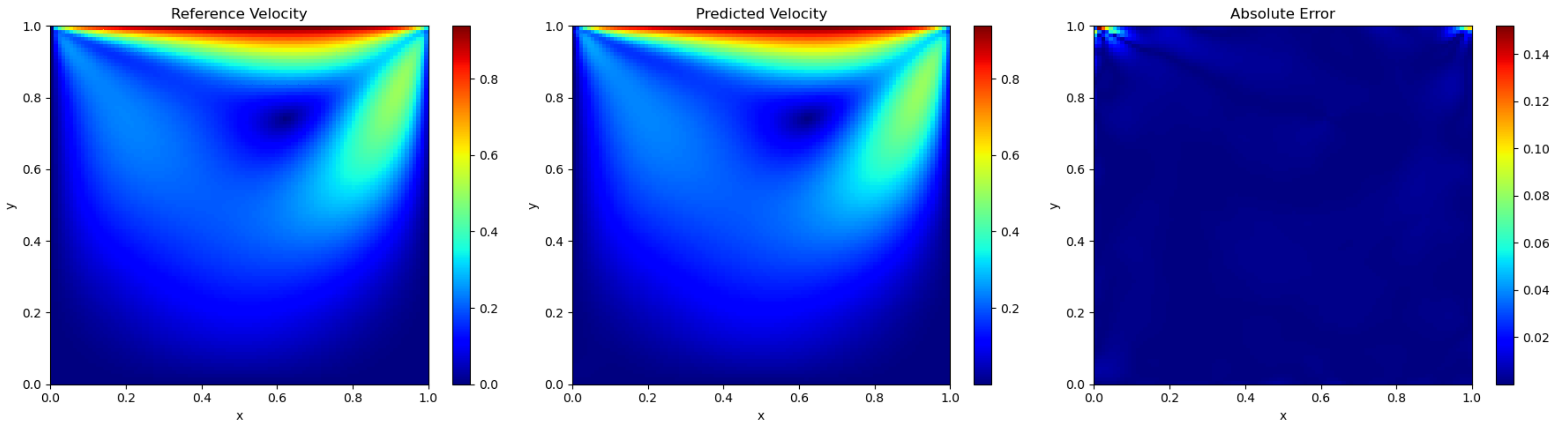
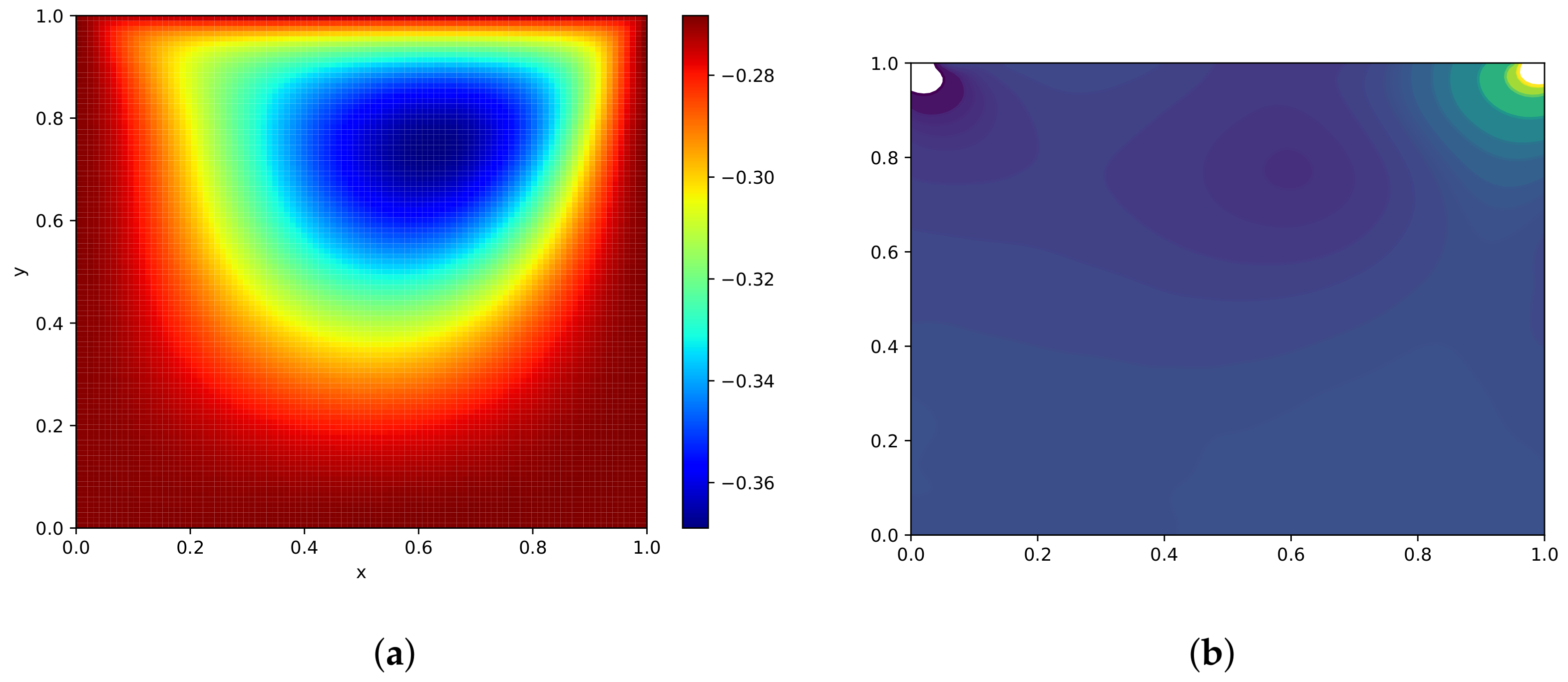
In this example, we use three wavelets in the wavelet-mapping layer. The followed fully connected neural network consists of three layers with 50 neurons in each layer. The training dataset contains $N_f = 2000$, $N_b = 200$. We first use the Adam method for 40,000 iterations and then use L-BFGS-B method for optimization. The relative $L^2$ error of velocity calculated in the end is $1.32 \times {10}^{-2}$. Figure 20 presents the reference velocity [60], predicted velocity and numerical error, respectively. It seems that the experimental result is in good agreement with reference result. Figure 21 shows the stream function $\psi$ and pressure p. A large vortex in the center of the square cavity can be observed.

3.3. High-Dimensional Equations

In this subsection, we consider two high-dimensional equations including Burgers equation and Poisson equation to show the validity and generalization ability of the proposed method.

3.3.1. Burgers Equation

We consider the three-dimensional time-dependent Burgers’ equation [54] as follows

$$\begin{array}{cc}\hfill & u_t + u{u}_x + v{u}_y + w{u}_z = \epsilon (u_{xx} + u_{yy} + u_{zz}),\hfill \end{array}$$

(77a)

$$\begin{array}{cc}\hfill & v_t + u{v}_x + v{v}_y + w{v}_z=\epsilon (v_{xx} + v_{yy} + v_{zz}),\hfill \end{array}$$

(77b)

$$\begin{array}{cc}\hfill & w_t + u{w}_x + v{w}_y + w{w}_z = \epsilon (w_{xx} + w_{yy} + w_{zz}),(x,y,z,t) \in {[a,b]}^3 \times [0,T].\hfill \end{array}$$

(77c)

The initial and boundary conditions are extracted from exact solutions, and the exact solutions are given by

$$\begin{array}{cc}\hfill & u(t,x,y,z) = -2\epsilon [{\displaystyle \frac{1 + e^{-t}cos\left(x\right)sin\left(y\right)sin\left(z\right)}{1 + x + e^{-t}sin\left(x\right)sin\left(y\right)sin\left(z\right)}}],\hfill \end{array}$$

(78a)

$$\begin{array}{cc}\hfill & v(t,x,y,z) = -2\epsilon [{\displaystyle \frac{e^{-t}sin\left(x\right)cos\left(y\right)sin\left(z\right)}{1 + x + e^{-t}sin\left(x\right)sin\left(y\right)sin\left(z\right)}}],\hfill \end{array}$$

(78b)

$$\begin{array}{cc}\hfill & w(t,x,y,z) = -2\epsilon [{\displaystyle \frac{e^{-t}sin\left(x\right)sin\left(y\right)cos\left(z\right)}{1 + x + e^{-t}sin\left(x\right)sin\left(y\right)sin\left(z\right)}}].\hfill \end{array}$$

(78c)

In this experiment, we set $\epsilon = 1$, $a = 0$, $b = 0.1$ and $T = 0.1$. To speed up the training process, we only use two wavelets in wavelet expansion layer and fed the enhanced pattern to a fully connected neural network with four hidden layers. Each hidden layer has 40 hidden neurons. It is noted that, three output nodes are needed to output u, v, w, respectively. The $f(t,x,y,z)$ is obtained from Equation (Section 3.3.1)

$$\begin{array}{cc}\hfill & f_1 := u_t + u{u}_x+v{u}_y + w{u}_z - \epsilon (u_{xx} + u_{yy} + u_{zz}),\hfill \end{array}$$

(79a)

$$\begin{array}{cc}\hfill & f_2 := v_t + u{v}_x + v{v}_y + w{v}_z - \epsilon (v_{xx} + v_{yy} + v_{zz}),\hfill \end{array}$$

(79b)

$$\begin{array}{cc}\hfill & f_3 := w_t + u{w}_x + v{w}_y + w{w}_z - \epsilon (w_{xx} + w_{yy} + w_{zz}).\hfill \end{array}$$

(79c)

Therefore, $f(t,x,y,z)$ is consist of three parts. The parameters are learned by minimizing the loss function $J\left(\theta \right)$

$$J\left(\theta \right) = MS{E}_f + MS{E}_{u,v,w} + MS{E}_{domain},$$

(80)

where

$$\begin{array}{cc}\hfill MS{E}_f = & \frac{1}{N_f}\sum _{i=1}^{N_f}{\left|f_1(t_f^i,x_f^i,y_f^i,z_f^i)\right|}^2 + \frac{1}{N_f}\sum _{i=1}^{N_f}{\left|f_2(t_f^i,x_f^i,y_f^i,z_f^i)\right|}^2 + \frac{1}{N_f}\sum _{i=1}^{N_f}{\left|f_3(t_f^i,x_f^i,y_f^i,z_f^i)\right|}^2,\hfill \end{array}$$

(81a)

$$\begin{array}{cc}\hfill MS{E}_{u,v,w} = & \frac{1}{N_{u,v,w}}\sum _{i=1}^{N_{u,v,w}}{|u(t_{u,v,w}^i,x_{u,v,w}^i,y_{u,v,w}^i,z_{u,v,w}^i) - u^i|}^2\hfill \\ \hfill & + \frac{1}{N_{u,v,w}}\sum _{i=1}^{N_{u,v,w}}{|v(t_{u,v,w}^i,x_{u,v,w}^i,y_{u,v,w}^i,z_{u,v,w}^i) - v^i|}^2\hfill \\ \hfill & + \frac{1}{N_{u,v,w}}\sum _{i=1}^{N_{u,v,w}}{|w(t_{u,v,w}^i,x_{u,v,w}^i,y_{u,v,w}^i,z_{u,v,w}^i) - w^i|}^2,\hfill \end{array}$$

(81b)

$$\begin{array}{cc}\hfill MS{E}_{domain} = & \frac{1}{N_{domain}}\sum _{i=1}^{N_{domain}}{|u(t_{domain}^i,x_{domain}^i,y_{domain}^i,z_{domain}^i) - u_{domain}^i|}^2\hfill \\ \hfill & + \frac{1}{N_{domain}}\sum _{i=1}^{N_{domain}}{|v(t_{domain}^i,x_{domain}^i,y_{domain}^i,z_{domain}^i) - v_{domain}^i|}^2\hfill \\ \hfill & + \frac{1}{N_{domain}}\sum _{i=1}^{N_{domain}}{|w(t_{domain}^i,x_{domain}^i,y_{domain}^i,z_{domain}^i) - w_{domain}^i|}^2.\hfill \end{array}$$

(81c)

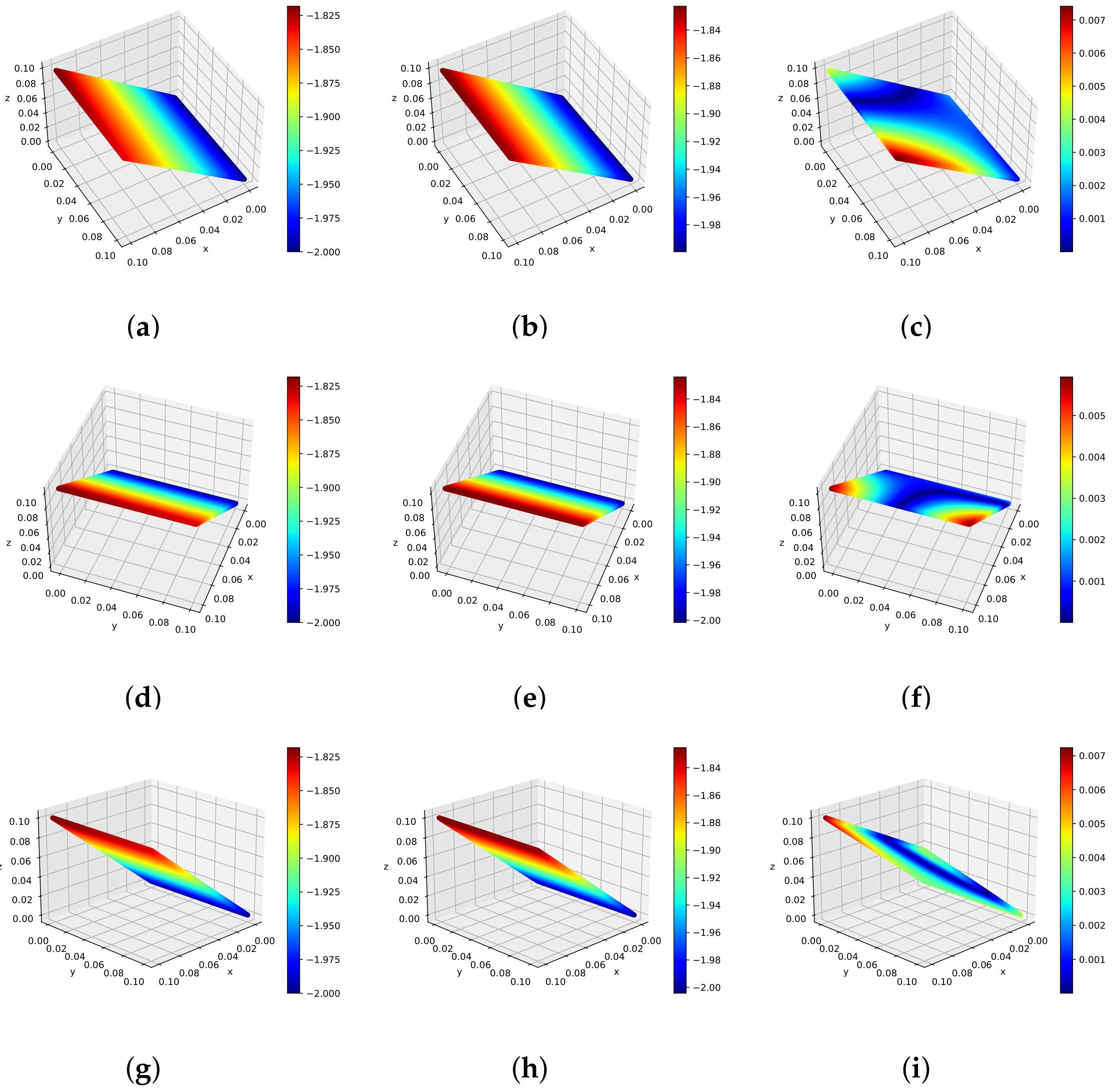
We randomly chose 200 initial/boundary training data points, 200 observations and 20,000 collocation points. The relative error was measured at $L^2$-norm is $1.16 \times {10}^{-3}$. We present the predicted result $u(t,x,y,z)$ from different perspectives. Figure 22 shows the exact solutions, predicted solutions, and absolute errors at different time instants. Figure 22a–c present the results at time $t = 0.01$. Figure 22d–f present the results at time $t = 0.05$. Finally, Figure 22g–i present the results at time $t = 0.1$. From Figure 22, we see that the prediction solutions are in satisfactory agreement with exact solutions.

3.3.2. Poisson Equation

We consider a Poisson equation with Dirichlet boundary condion [61]

$$\left\{\begin{array}{c}-\Delta u = {\displaystyle \frac{{\pi }^2}{4}}\sum _{i=1}^{d}sin({\displaystyle \frac{\pi }{2}}{\mathit{x}}_{\mathit{i}}),\mathrm{\Omega } = {(0,1)}^d,\hfill \\ u = \sum _{i=1}^{d}sin({\displaystyle \frac{\pi }{2}}{\mathit{x}}_{\mathit{i}}),on\partial \mathrm{\Omega }\hfill \end{array}\right.$$

(82)

with problem dimension $d = 5$. The classical solution for this problem is $u(\mathit{x}) = \sum _{i=1}^{d}sin({\displaystyle \frac{\pi }{2}}{\mathit{x}}_{\mathit{i}})$.

We also use two wavelets in wavelet expansion layer in this part. The followed fully connected network is considered to five hidden layers, and each hidden layer uses 40 neurons. The $f\left(\mathit{x}\right)$ is obtained from Equation (82)

$$f := -\Delta u - {\displaystyle \frac{{\pi }^2}{4}}\sum _{i=1}^{d}sin({\displaystyle \frac{\pi }{2}}{\mathit{x}}_{\mathit{i}}).$$

(83)

The optimal parameters are trained by minimizing loss function $J\left(\theta \right)$

$$J\left(\theta \right) = MS{E}_f + MS{E}_u,$$

(84)

where

$$MS{E}_f = \frac{1}{N_f}\sum _{i=1}^{N_f}{\left|f({\mathit{x}}_{\mathit{f}}^{\mathit{i}})\right|}^2,$$

(85)

$$MS{E}_u = \frac{1}{N_u}\sum _{i=1}^{N_u}{|u\left({\mathit{x}}_{\mathit{u}}^{\mathit{i}}\right) - u^i|}^2.$$

(86)

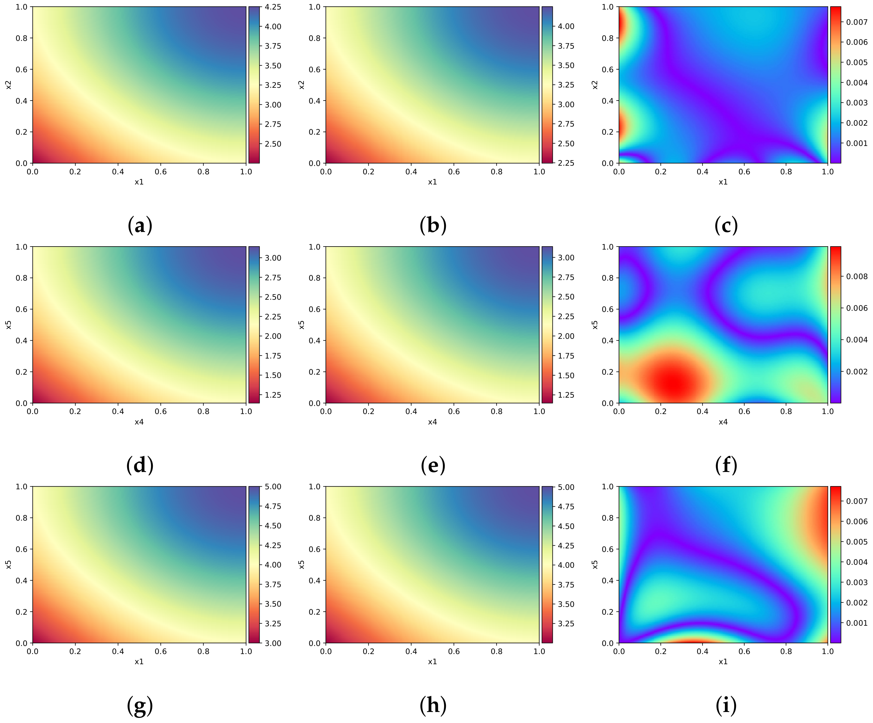
The training data set includes initial/boundary points $N_u = 150$ and collocation points $N_f$ = 20,000, respectively. The relative $L^2$ error calculated is $1.76 \times {10}^{-3}$. Figure 23 shows the analytical solutions, numerical solutions and absolute errors in the different planes. Figure 23a–c shows the plane $x_1 \circ x_2$, when $x_3 = 0.9$, $x_4 = 0.6$, $x_5 = 0.3$. Figure 23d–f shows the plane $x_4 \circ x_5$, when $x_1 = 0.9$, $x_2 = 0.09$, $x_3 = 0.009$. Finally, Figure 23g–i shows the plane $x_1 \circ x_5$, when $x_2 = 1$, $x_3 = 1$, $x_4 = 1$. From the Figure 23, we observe that the simulation results are in excellent agreement with the exact solutions.

3.4. Comparison of DWNN and Others

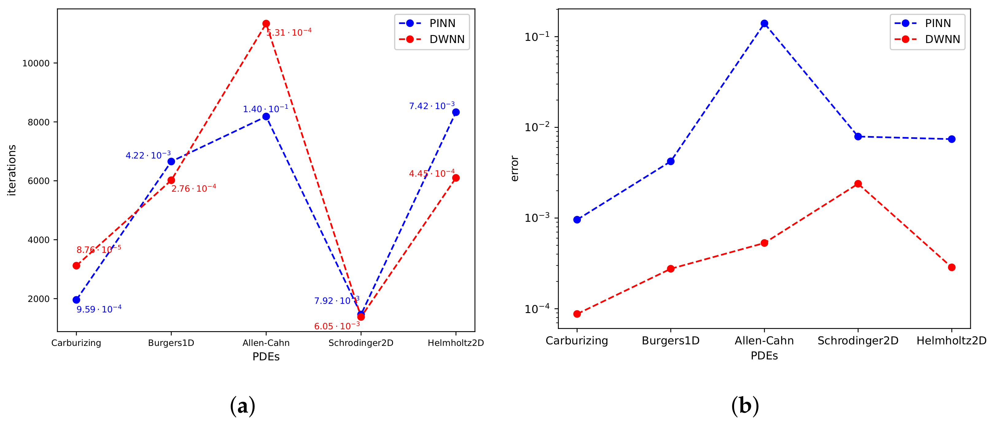
To demonstrate the merit of the proposed DWNN model, we present the number of iterations and the relative $L^2$ errors of PINN and DWNN for five numerical examples including the carburizing diffusion equation, 1D Burgers equation, Allen-Cahn equation, 2D Schrödinger equation, and 2D Helmholtz equation. Figure 24a shows the number of iterations of PINN and DWNN, and the corresponding relative $L^2$ error is marked near each data point. First, we use five wavelets to solve the carburizing diffusion equation and Burgers equation. As we can see from Figure 24a, there is little difference in the number of iterations between PINN and DWNN for these two cases. However, the relative $L^2$ error of DWNN model is one order of magnitude lower than that of PINN. Second, we solve the Allen-Cahn equation using five wavelets and add a small sample of observations to the training set; finally, the DWNN model has 3155 more iterations than PINN. However, meanwhile, the relative $L^2$ error of DWNN is almost three orders of magnitude lower than PINN. Lastly, we use three wavelets to solve the Helmholtz equation in two-dimensions. Because fewer wavelets are used, the number of features increases slightly. Therefore, the results show that in the training process of two-dimensional Helmholtz equation, the DWNN model has fewer iterations and higher predictive accuracy. Figure 24b shows the comparison of relative $L^2$ errors between PINN and DWNN for five examples, from which we observe that DWNN model achieves a higher predictive accuracy. The more intuitive relative $L_2$ error results for DeLISA [62], Deep learning-based method coupled with SSL [31] (For brevity, denoted as SSL), and DWNN are listed in

Table 10. The comparison of different methods with respect to relative $L^2$ errors.

PDE	DeLISA	SSL	DWNN
1D-Schrödinger	$1.43 \times {10}^{-3}$	$6.87 \times {10}^{-4}$	$5.04 \times {10}^{-4}$
Carburizing	$2.70 \times {10}^{-4}$	$5.93 \times {10}^{-4}$	$8.76 \times {10}^{-5}$
1D-Burgers	$3.18 \times {10}^{-3}$	$5.50 \times {10}^{-4}$	$2.76 \times {10}^{-4}$
Allen-Cahn	$7.25 \times {10}^{-3}$	$8.98 \times {10}^{-3}$	$5.31 \times {10}^{-4}$
2D-Burgers	$8.51 \times {10}^{-5}$	$2.70 \times {10}^{-4}$	$3.25 \times {10}^{-4}$
2D-Schrödinger	$5.06 \times {10}^{-2}$	$1.30 \times {10}^{-3}$	$2.39 \times {10}^{-3}$

. For the cases in Table 10, we show the optimal solution with respect to the different methods. The results suggest that DWNN model performs better overall.

4. Discussion

In this work, we propose a deep wavelet neural network to tackle a series of partial differential equations. To gain further insight, we record and compare the experimental results of DWNN model and other state-of-the-art algorithms respectively. We also present experiments to validate the effectiveness of each part of the proposed model. Taken together, the development of this work provides a new architecture and training algorithm to improve the generalization ability and predictive accuracy significantly. Moreover, the proposed model is also good at solving shock-wave problems and interface problems. Despite these advances, we must acknowledge that one limitation of the proposed architecture is that we must carefully choose the number of appropriate wavelet mappings. At present, our system tends to be stable when the number of wavelets is near five. There are also many open questions worth considering as future research directions. Can we strictly establish a universal optimal design and its theory? Can we design other useful feature embedding to handle different scenarios? We believe that answering these questions not only leads to a better understanding of network models, but also opens a new door for developing interpretable machine learning algorithms that are necessary for many key applications in science and engineering.

5. Conclusions

In this paper, we propose a deep wavelet neural network model to solve partial differential equations. We introduce wavelets to the deep architecture to obtain a fine feature description and extraction. Then we use Gaussian error activation function instead of other traditional activation functions. Moreover, we add a tunable residual term of a few sample data points into the cost function to rectify the model. To investigate the performance of the proposed method, we carry out a variety of numerical experiments including Schrödinger equation, carburizing equation, Klein-Gordon equation, Burgers equation, Allen-Cahn equation, Helmholtz equation, and Poisson equation. In all cases, the relative $L^2$ error and $L^{\infty }$ error in solution are shown to be smaller than the state-of-the-art approach. We also present ablation experiments to validate the effectiveness of each part of the proposed model. The numerical results verify that the proposed method improves the predictive accuracy, robustness, and generalization ability.

References

Ricardo, H.J. A Modern Introduction to Differential Equations; Academic Press: Cambridge, MA, USA, 2020. [Google Scholar]
Eymard, R.; Gallouët, T.; Herbin, R. Finite volume methods. In Handbook of Numerical Analysis; Elsevier: Amsterdam, The Netherlands, 2000; Volume 7, pp. 713–1018. [Google Scholar]
Zhang, Y. A finite difference method for fractional partial differential equation. Appl. Math. Comput.2009, 215, 524–529. [Google Scholar] [CrossRef]
Taylor, C.A.; Hughes, T.J.; Zarins, C.K. Finite element modeling of blood flow in arteries. Comput. Methods Appl. Mech. Eng.1998, 158, 155–196. [Google Scholar] [CrossRef]
Du, Y.; Wang, W.; Wang, L. Hierarchical recurrent neural network for skeleton based action recognition. In Proceedings of the IEEE Conference on Computer Vision And Pattern Recognition, Boston, MA, USA, 7–12 June 2015; pp. 1110–1118. [Google Scholar]
Feichtenhofer, C.; Pinz, A.; Zisserman, A. Convolutional two-stream network fusion for video action recognition. In Proceedings of the IEEE Conference on Computer Vision and Pattern Recognition, Las Vegas, NV, USA, 27–30 June 2016; pp. 1933–1941. [Google Scholar]
Lagaris, I.E.; Likas, A.C.; Papageorgiou, D.G. Neural-network methods for boundary value problems with irregular boundaries. IEEE Trans. Neural Netw.2000, 11, 1041–1049. [Google Scholar] [CrossRef] [Green Version]
Mai-Duy, N.; Tran-Cong, T. Numerical solution of differential equations using multiquadric radial basis function networks. Neural Netw.2001, 14, 185–199. [Google Scholar] [CrossRef] [Green Version]
Mai-Duy, N.; Tran-Cong, T. Approximation of function and its derivatives using radial basis function networks. Appl. Math. Model.2003, 27, 197–220. [Google Scholar] [CrossRef] [Green Version]
Pao, Y.H.; Phillips, S.M. The functional link net and learning optimal control. Neurocomputing1995, 9, 149–164. [Google Scholar] [CrossRef]
Mall, S.; Chakraverty, S. Application of Legendre neural network for solving ordinary differential equations. Appl. Soft Comput.2016, 43, 347–356. [Google Scholar] [CrossRef]
Mall, S.; Chakraverty, S. Single layer Chebyshev neural network model for solving elliptic partial differential equations. Neural Process. Lett.2017, 45, 825–840. [Google Scholar] [CrossRef]
Sun, H.; Hou, M.; Yang, Y.; Zhang, T.; Weng, F.; Han, F. Solving partial differential equation based on Bernstein neural network and extreme learning machine algorithm. Neural Process. Lett.2019, 50, 1153–1172. [Google Scholar] [CrossRef]
Weinan, E.; Han, J.; Jentzen, A. Deep learning-based numerical methods for high-dimensional parabolic partial differential equations and backward stochastic differential equations. Commun. Math. Stat.2017, 5, 349–380. [Google Scholar]
Han, J.; Weinan, E. Deep learning approximation for stochastic control problems. arXiv2016, arXiv:1611.07422. [Google Scholar]
Han, J.; Jentzen, A.; Weinan, E. Solving high-dimensional partial differential equations using deep learning. Proc. Natl. Acad. Sci. USA2018, 115, 8505–8510. [Google Scholar] [CrossRef] [Green Version]
Han, J.; Zhang, L.; Weinan, E. Solving many-electron Schrödinger equation using deep neural networks. J. Comput. Phys.2019, 399, 108929. [Google Scholar] [CrossRef] [Green Version]
Sirignano, J.; Spiliopoulos, K. DGM: A deep learning algorithm for solving partial differential equations. J. Comput. Phys.2018, 375, 1339–1364. [Google Scholar] [CrossRef] [Green Version]
Zang, Y.; Bao, G.; Ye, X.; Zhou, H. Weak adversarial networks for high-dimensional partial differential equations. J. Comput. Phys.2020, 411, 109409. [Google Scholar] [CrossRef] [Green Version]
Raissi, M.; Perdikaris, P.; Karniadakis, G.E. Physics-informed neural networks: A deep learning framework for solving forward and inverse problems involving nonlinear partial differential equations. J. Comput. Phys.2019, 378, 686–707. [Google Scholar] [CrossRef]
Jagtap, A.D.; Kharazmi, E.; Karniadakis, G.E. Conservative physics-informed neural networks on discrete domains for conservation laws: Applications to forward and inverse problems. Comput. Methods Appl. Mech. Eng.2020, 365, 113028. [Google Scholar] [CrossRef]
Mallat, S.; Zhong, S. Characterization of signals from multiscale edges. IEEE Trans. Pattern Anal. Mach. Intell.1992, 14, 710–732. [Google Scholar] [CrossRef] [Green Version]
Zainuddin, Z.; Pauline, O. Modified wavelet neural network in function approximation and its application in prediction of time-series pollution data. Appl. Soft Comput.2011, 11, 4866–4874. [Google Scholar] [CrossRef]
Liu, H.; Mi, X.w.; Li, Y.f. Wind speed forecasting method based on deep learning strategy using empirical wavelet transform, long short term memory neural network and Elman neural network. Energy Convers. Manag.2018, 156, 498–514. [Google Scholar] [CrossRef]
Wang, C.; Gao, R.X. Wavelet transform with spectral post-processing for enhanced feature extraction. In Proceedings of the 19th IEEE Instrumentation and Measurement Technology Conference (IEEE Cat. No. 00CH37276) IMTC/2002, Anchorage, AK, USA, 21–23 May 2002; Volume 1, pp. 315–320. [Google Scholar]
Li, Y.; Mei, F. Deep learning-based method coupled with small sample learning for solving partial differential equations. Multimed. Tools Appl.2021, 80, 17391–17413. [Google Scholar] [CrossRef]
Ososkov, G.; Shitov, A. Gaussian wavelet features and their applications for analysis of discretized signals. Comput. Phys. Commun.2000, 126, 149–157. [Google Scholar] [CrossRef]
Berkani, M.S.; Giurgea, S.; Espanet, C.; Coulomb, J.L.; Kieffer, C. Study on optimal design based on direct coupling between a FEM simulation model and L-BFGS-B algorithm. IEEE Trans. Magn.2013, 49, 2149–2152. [Google Scholar] [CrossRef]
Andrews, L.C. Special Functions of Mathematics for Engineers; Spie Press: Bellingham, WA, USA, 1998; Volume 49. [Google Scholar]
Chen, T.; Chen, H. Universal approximation to nonlinear operators by neural networks with arbitrary activation functions and its application to dynamical systems. IEEE Trans. Neural Netw.1995, 6, 911–917. [Google Scholar] [CrossRef] [Green Version]
Lanthaler, S.; Mishra, S.; Karniadakis, G.E. Error estimates for deeponets: A deep learning framework in infinite dimensions. Trans. Math. Its Appl.2022, 6, tnac001. [Google Scholar] [CrossRef]
Lu, L.; Jin, P.; Pang, G.; Zhang, Z.; Karniadakis, G.E. Learning nonlinear operators via DeepONet based on the universal approximation theorem of operators. Nat. Mach. Intell.2021, 3, 218–229. [Google Scholar] [CrossRef]
Baydin, A.G.; Pearlmutter, B.A.; Radul, A.A.; Siskind, J.M. Automatic differentiation in machine learning: A survey. J. Mach. Learn. Res.2018, 18, 1–43. [Google Scholar]
Sun, Z. A meshless symplectic method for two-dimensional nonlinear Schrödinger equations based on radial basis function approximation. Eng. Anal. Bound. Elem.2019, 104, 1–7. [Google Scholar] [CrossRef]
Schrödinger, E. An undulatory theory of the mechanics of atoms and molecules. Phys. Rev.1926, 28, 1049. [Google Scholar] [CrossRef]
Stein, M. Large sample properties of simulations using Latin hypercube sampling. Technometrics1987, 29, 143–151. [Google Scholar] [CrossRef]
Platte, R.B.; Trefethen, L.N. Chebfun: A new kind of numerical computing. In Progress in Industrial Mathematics at ECMI 2008; Springer: Berlin/Heidelberg, Germany, 2010; pp. 69–87. [Google Scholar]
Kingma, D.P.; Ba, J. Adam: A method for stochastic optimization. arXiv2014, arXiv:1412.6980. [Google Scholar]
Maisuradze, M.V.; Kuklina, A.A. Numerical solution of the differential diffusion equation for a steel carburizing process. In Solid State Phenomena; Trans Tech Publications Ltd.: Freienbach, Switzerland, 2018; Volume 284, pp. 1230–1234. [Google Scholar]
Kula, P.; Pietrasik, R.; Dybowski, K. Vacuum carburizing—Process optimization. J. Mater. Process. Technol.2005, 164, 876–881. [Google Scholar] [CrossRef]
Xia, C.; Li, Y.; Wang, H. Local discontinuous Galerkin methods with explicit Runge-Kutta time marching for nonlinear carburizing model. Math. Methods Appl. Sci.2018, 41, 4376–4390. [Google Scholar] [CrossRef]
Caudrey, P.; Eilbeck, J.; Gibbon, J. The sine-Gordon equation as a model classical field theory. Il Nuovo Cimento B (1971–1996)1975, 25, 497–512. [Google Scholar] [CrossRef]
Dodd, R.K.; Morris, H.C.; Eilbeck, J.; Gibbon, J. Soliton and nonlinear wave equations. London and New York. 1982. Available online: https://www.osti.gov/biblio/6349564 (accessed on 25 April 2022).
Wazwaz, A.M. New travelling wave solutions to the Boussinesq and the Klein-Gordon equations. Commun. Nonlinear Sci. Numer. Simul.2008, 13, 889–901. [Google Scholar] [CrossRef]
Jagtap, A.D.; Kawaguchi, K.; Karniadakis, G.E. Adaptive activation functions accelerate convergence in deep and physics-informed neural networks. J. Comput. Phys.2020, 404, 109136. [Google Scholar] [CrossRef] [Green Version]
Basdevant, C.; Deville, M.; Haldenwang, P.; Lacroix, J.; Ouazzani, J.; Peyret, R.; Orlandi, P.; Patera, A. Spectral and finite difference solutions of the Burgers equation. Comput. Fluids1986, 14, 23–41. [Google Scholar] [CrossRef]
Bateman, H. Some recent researches on the motion of fluids. Mon. Weather Rev.1915, 43, 163–170. [Google Scholar] [CrossRef]
Yang, X.; Ge, Y.; Zhang, L. A class of high-order compact difference schemes for solving the Burgers’ equations. Appl. Math. Comput.2019, 358, 394–417. [Google Scholar] [CrossRef]
Allen, S.M.; Cahn, J.W. A microscopic theory for antiphase boundary motion and its application to antiphase domain coarsening. Acta Metall.1979, 27, 1085–1095. [Google Scholar] [CrossRef]
Beneš, M.; Chalupeckỳ, V.; Mikula, K. Geometrical image segmentation by the Allen-Cahn equation. Appl. Numer. Math.2004, 51, 187–205. [Google Scholar] [CrossRef]
Dobrosotskaya, J.A.; Bertozzi, A.L. A wavelet-Laplace variational technique for image deconvolution and inpainting. IEEE Trans. Image Process.2008, 17, 657–663. [Google Scholar] [CrossRef]
Feng, X.; Prohl, A. Numerical analysis of the Allen-Cahn equation and approximation for mean curvature flows. Numer. Math.2003, 94, 33–65. [Google Scholar] [CrossRef]
Wheeler, A.A.; Boettinger, W.J.; McFadden, G.B. Phase-field model for isothermal phase transitions in binary alloys. Phys. Rev. A1992, 45, 7424. [Google Scholar] [CrossRef]
Wang, S.; Teng, Y.; Perdikaris, P. Understanding and mitigating gradient flow pathologies in physics-informed neural networks. SIAM J. Sci. Comput.2021, 43, A3055–A3081. [Google Scholar] [CrossRef]
Yu, B. The deep Ritz method: A deep learning-based numerical algorithm for solving variational problems. Commun. Math. Stat.2018, 6, 1–12. [Google Scholar]
Li, Y.; Zhou, Z.; Ying, S. DeLISA: Deep learning based iteration scheme approximation for solving PDEs. J. Comput. Phys.2022, 451, 110884. [Google Scholar] [CrossRef]
Figure 1.
Architecture of deep wavelet neural network.
Figure 3.
The comparison of activation function. (a) Sigmoid and ReLu. (b) ERF and Tanh.
Figure 4.
Diagram of Gaussian error function and its derivative. (a) Gaussian error function. (b) The derivative of the Gaussian error function.
Figure 5.
Results of Equation (22). (a) The predicted solution . (b) The change process of the objective function versus iteration number.
Figure 6.
Comparison of predicted solution and exact solution of Equation (22) corresponding to different temporal snapshots. (a) ; (b) ; (c) ; (d) .
Figure 7.
Results of Equation (28). (a) The predicted solution . (b) The change process of the objective function versus iteration number.
Figure 8.
Comparison of predicted solution and exact solution of Equation (28) corresponding to different temporal snapshots. (a) ; (b) ; (c) ; (d) .
Figure 9.
Results of Equation (34). (a) The predicted solution . (b) The change process of the objective function versus iteration number.
Figure 10.
Comparison of predicted solution and exact solution of Equation (34) corresponding to different x. (a) ; (b) ; (c) ; (d) .
Figure 11.
Results of Equation (39). (a) The predicted solution . (b) The change process of the objective function versus iteration number.
Figure 12.
The Loss and error of Burgers and Allen-Cahn. (a) 1D Burgers. (b) Allen-Cahn.
Figure 13.
Comparison of predicted solution and exact solution of Equation (39) corresponding to different temporal snapshots. (a) ; (b) ; (c) ; (d) .
Figure 14.
Results of Equation (45). (a) The predicted solution . (b) The change process of the objective function versus iteration number.
Figure 15.
Comparison of predicted solution and exact solution of Equation (45) based on PINN, WTNN and DWNN. (a–c) the comparison of predicted PINN solution, WTNN solution, DWNN solution and exact solution at , respectively. (d–f) the comparison of predicted PINN solution, WTNN solution, DWNN solution and exact solution at , respectively.
Figure 16.
Results of Equation (52). (a) Exact solution at time . (b) Predicted solution at time . (c) Numerical error at time . (d) The change process of the objective function versus iteration number.
Figure 17.
Results of Equation (58). (a) Exact solution at time . (b) Predicted solution at time . (c) Numerical error at time . (d) Loss vs. iterations.
Figure 18.
Results of Equation (64). (a) The predicted solution . (b) The change process of the objective function versus iteration number.
Figure 19.
Comparison of predicted solution and exact solution of Equation (64) at different x. (a) ; (b) ; (c) ; (d) .
Figure 21.
The stream function and pressure field p. (a) The stream function . (b) Pressure field p.
Figure 22.
Results of Equation (Section 3.3.1) at different time instants. (a–c) Exact solution, numerical solution, and numerical error at . (d–f) Exact solution, numerical solution, and numerical error at . (g–i) Exact solution, numerical solution, and numerical error at .
Figure 23.
Results of Equation (82) in the different planes. (a–c) Exact solution, numerical solution and numerical error in the plane , . (d–f): Exact solution, numerical solution and numerical error in the plane , . (g–i) Exact solution, numerical solution and numerical error in the plane , .
Figure 24.
The comparison of iterations and errors. (a) Iteration comparison. (b) Error comparison.