An Image Encryption Scheme Synchronizing Optimized Chaotic Systems Implemented on Raspberry Pis

Abstract

Guaranteeing security in information exchange is a challenge in public networks, such as in the highly popular application layer Message Queue Telemetry Transport (MQTT) protocol. On the one hand, chaos generators have shown their usefulness in masking data that can be recovered while having the appropriate binary string. Privacy can then be accomplished by implementing synchronization techniques to connect the transmitter and receiver, among millions of users, to encrypt and decrypt data having the correct public key. On the other hand, chaotic binary sequences can be generated on Rapsberry Pis that can be connected over MQTT. To provide privacy and security, the transmitter and receiver (among millions of devices) can be synchronized to have the same chaotic public key to encrypt and decrypt data. In this manner, this paper shows the implementation of optimized chaos generators on Raspberry Pis that are wirelessly connected via MQTT for the IoT protocol. The publisher encrypts data that are public to millions of interconnected devices, but the data are decrypted by the subscribers having the correct chaotic binary sequence. The image encryption system is tested by performing NIST, TestU01, NPCR, UACI and other statistical analyses.

1. Introduction

From the seminal work of Lorenz [1], chaos theory has shown advantages in the design of secure communication systems to mask [2] and encrypt information [3,4,5,6,7]. Nowadays, chaos theory is an interdisciplinary branch that states the interconnections, feedback loops, patterns, repetition, fractals, self-similarity and self-organization in complex systems regardless of the apparent randomness [8]. The main property of a chaotic system is often related to the high sensitivity of the system’s response to the initial conditions (i.e., small changes can lead to significant differences in the dynamics of the chaotic system).

Recent applications of chaotic systems include the development of optimization methods [8] and the design of privacy-enhanced communication protocols for lightweight Internet of Things (IoT) devices [9]. As mentioned in [10], security is a key problem for the transmission, interchange and storage process of multimedia systems and applications, so research efforts have been focused on this open problem. On the side of ubiquitous sensing in public and wireless networks, data protection is a challenge in IoT applications, in which a connected device publishes data that are read by millions of interconnected heterogeneous and pervasive devices. The MQTT communication approach is based on a publish–subscribe model (https://mqtt.org/ (accessed on 1 March 2022)), where neither have notions about the existence of the other and rely on a third party, called the broker, who distributes the messages to all connected devices. Therefore, the publisher only needs to send its data once without knowing how many subscribers will be served by the broker. For instance, the authors in [11] used fractional-order chaotic maps for secure communication in IoT-based smart devices. Fractional-order chaotic systems can be synchronized, but recent works just synchronized master–slave topologies [12,13]. The challenge is synchronizing any number of devices to share secure data on public networks and guaranteeing privacy. Herein, we propose the use of chaotic binary strings to synchronize a publisher (transmitter) with any number of subscribers (receivers) so that the data can be recovered just by the subscriber having the correct chaotic binary string (public key), while the remaining connected devices can read a kind of noisy data.

Chaotic systems have been implemented in different analog and digital electronic devices [7], and in both cases, the exactness depends on the numerical method or approximation to solve the fractional-order derivatives. This paper shows the implementation of chaotic systems using Raspberry Pis (RPis) to exploit their computer-on-board capabilities. In this manner, each RPi is ready to generate chaotic binary strings to encrypt and decrypt an image that can be processed wirelessly over MQTT for the IoT protocol. Chaotic systems can also be designed using integrated circuit technology, as shown in [14,15,16,17]. The challenges are related to the design of low-power IoT devices for lightweight applications and the development of secure and private communication systems. In this manner, to guarantee privacy, this paper shows the synchronization of a publisher (transmitter) with multiple subscribers (receivers) using chaotic binary strings in MQTT for the IoT protocol. We also perform National Institute of Standards and Technology (NIST) and TestU01 tests to guarantee the randomness of the chaotic binary strings and perform other statistical analyses to avoid attacks for the encryption and decryption of images. The encryption system is implemented using IoT devices such as RPis.

The rest of the paper is organized as follows. Section 2 summarizes the classification of chaotic systems and their optimization and describes the generation of random binary strings that are verified by NIST and TestU01 tests. Section 3 shows the synchronization of optimized chaotic systems by applying two methods: Hamiltonian forms and the observer approach, which is given in Section 3.1, and the OPCL synchronization method, given in Section 3.2. The hardware implementation of an image encryption system in MQTT based on Raspberry Pis is given in Section 4, where some images are encrypted and analyzed. Finally, the conclusions are summarized in Section 5.

2. Chaotic Systems and Random Binary Strings

Chaotic systems are modeled by ordinary differential equations (ODEs), which can be of an integer or fractional order. The dynamical characteristics can be measured by evaluating the Lyapunov exponents (LEs) and Kaplan–Yorke dimension $D_{KY}$. For systems having three ODEs, one can evaluate three LEs, with one being negative, one being zero (or very close to zero) and one being positive. Chaotic behavior exists if the system has one positive LE. For systems having more than three ODEs, one can evaluate more than one positive LE, where the highest is known as the maximum LE (MLE) and the system is said to have hyperchaotic behavior. The chaotic time series associated to each state variable can be transformed to binary strings whose randomness is measured by statistical tests such as NIST and TestU01.

Sprott published a collection of chaotic systems consisting of three ODEs, where the nonlinearity is given by multiplying two state variables and having a low number of coefficients [18]. Other well-known chaotic systems having three ODEs are the Lorenz, Rössler, Chua, Chen and Lü systems. If the ODEs have defined and unique equilibrium points, the system generates self-excited attractors; otherwise, hidden attractors exist. However, the ODEs have particular parameter values to generate chaotic behavior [19], and those values can be found by generating bifurcation diagrams. The initial conditions must also be close to the equilibrium point or the attraction region to generate a chaotic attractor. In all published works, the authors provide the parameter values the initial conditions of a mathematical model to reproduce chaotic behavior. However, one may get different chaotic behavior depending on the numerical method and step size h that is used [20]. Once a chaotic system is solved by a numerical method, the time series can be used to evaluate the LE spectrum and $D_{KY}$. The mathematical model can be used to evaluate these characteristics by applying Wolf’s method [21]. That aside, if one has experimental chaotic time series, one can use the free software called time series analysis (TISEAN (https://www.pks.mpg.de/tisean/Tisean_3.0.1/index.html, accessed on 1 March 2022)) to estimate the LE spectrum and $D_{KY}$ [22]. Considering the chaotic Chen system given in Equation (1), and by setting $a=35.0$, $b=3.0$ and $c=28.0$, one can find three equilibrium points: $E{P}_1$ located at $x_1=x_2=7.9372$ and $x_3=21.0$, $E{P}_2$ located at $x_1=x_2=-7.9372$ and $x_3=21.0$ and $E{P}_3$ at $x_1=0,x_2=0$ and $x_3=0$. These $EP$s are used to evaluate the Jacobian and find the eigenvalues in order to verify the stabilized regions [20]:

$$\begin{array}{c}\dot{x_1}=a(x_2-x_1),\hfill \\ \dot{x_2}=(c-a)x_1-x_1{x}_3+c{x}_2,\hfill \\ \dot{x_3}=x_1{x}_2-b{x}_3.\hfill \end{array}$$

(1)

Mathematically speaking, all integer-order chaotic systems, such as the one given in Equation (1), can be transformed to their fractional-order versions. In this case, the fractional-order Chen system can be denoted by Equation (2), which generates chaotic behavior if $a=35,b=3,c=28$ and the fractional orders $q_1=q_2=q_3=0.96$. The system can be simulated by applying the Grünwald–Letnikov method with the initial conditions ${x_1}_0={x_2}_0={x_3}_0=0.01$, $h=0.001$ and memory length L = 32. The LEs are evaluated by TISEAN and are equal to LE${}_1$ = 3.5317, LE${}_2$ = 0.0037 and LE${}_3$ = −21.379. Furthermore, $D_{KY}$ = 2.1654, thus confirming chaotic behavior:

$$\begin{array}{c}{D}_t^{q_1}{x}_1=a(x_2-x_1),\hfill \\ D_t^{q_2}{x}_2=(c-a)x_1-x_1{x}_3+c{x}_2,\hfill \\ D_t^{q_3}{x}_3=x_1{x}_2-b{x}_3.\hfill \end{array}$$

(2)

Both integer- and fractional-order chaotic systems can be optimized by applying metaheuristics, as shown in [23], in order to increase the randomness to improve its application in image encryption, as detailed in the following sections. However, finding the parameters that generate chaotic behavior is not a trivial task, and the challenge is formulating the problem to be solved in an intuitive fashion (e.g., applying heuristics [24]), where the solutions provide acceptable values for the objective functions in either mono-objective or multi-objective optimization [25,26]. For instance, the non-dominated sorting genetic algorithm (NSGA-II) has been adopted as one of the best multi-objective algorithms [27]. In this work, it was applied to two objective functions: maximizing MLE and $D_{KY}$, both of which are in conflict and can be ranked on the Pareto front.

According to [23], the Chen system is optimized by NSGA-II, and

Table 1. Optimization results of Equation (1) applying NSGA-II, listing the non-optimized parameters in the first row and five optimal solutions taken from the Pareto front shown in Figure 1.

a	b	c	LE+	${\mathit{D}}_{\mathit{K}\mathit{Y}}$
35.0	3.0	28.0	2.0440	2.1698
35.514979	2.6385232	27.582793	2.6800429	2.2042597
35.488084	2.6193955	27.584261	2.6794532	2.2050013
33.532833	1.4708819	27.400097	2.4047606	2.2425449
33.0	1.2355012	27.714443	2.2429468	2.2592703
33.0	1.0910769	27.836426	2.2172809	2.2663249

shows the non-optimized values of Equation (1) in the first row ($a=35,b=3$ and $c=28$, while LE+ = 2.0440 and $D_{KY}$ = 2.1698) and five optimal solutions from rows 2 to 6. The complete Pareto front using an initial population of 120 individuals for 100 generations is shown in Figure 1. The parameters were set in the ranges a in [33.0,45.0], b in [0.1,5.0] and c in [20.0,28.0]. Figure 2 shows the attractors of the six cases given in Table 1.

The chaotic time series can be used to generate random binary strings, in which the challenge is guaranteeing the randomness. This work applies MOD255 to convert the real values to binary values. In this case, the sampling period is estimated by applying the autocorrelation function to the chaotic time series [28]. This analysis increases the entropy [29]. Figure 3a shows the autocorrelation of $x_1$ in the Chen system, and Figure 3b details the first zero crossing at iteration 127, meaning that one can sample every 127 iterations, and the real value is multiplied by a large number (in this work, 10,000,000). Finally, by applying MOD255, one obtains 8 bits (bytes) that are concatenated to the next ones to generate the random binary string that is used to encrypt images, as detailed in the next sections.

The randomness of the binary strings is evaluated herein by performing two statistical tests, namely NIST [30] and TestU01 [31]. Considering the fractional-order Chen system in Equation (2), whose optimized parameters are a = 39.2601, b = 3.2218 and c = 29.7607, we performed NIST tests for two cases. The first case consisted of 100 binary strings of 1,000,000 bits, and the second had the same binary string, but we applied post-processing with XOR operations for every 5 bits [32].

Table 2. NIST tests of the binary sequences from the fractional-order Chen system in Equation (2) using optimized parameters (a = 39.2601, b = 3.2218 and c = 29.7607) and without and with XOR post-processing. The symbol “*” means that the test was unsatisfactory, so one can see that the randomness was successful when applying XOR post-processing.

Statistical Test	p-Value without XOR	Proportion without XOR	p-Value with XOR	Proportion with XOR
Frequency	0.021932	96/100	0.657933	99/100
BlockFrequency	0.494136	98/100	0.319084	98/100
CumulativeSums	0.002230	87/100 *	0.236810	99/100
CumulativeSums	0.002357	95/100 *	0.455937	99/100
Runs	0.797481	99/100	0.137282	99/100
LongestRun	0.887251	100/100	0.657933	99/100
FFT	0.192597	99/100	0.616305	99/100
ApproximateEntropy	0.977971	100/100	0.000555	98/100
Serial	0.076439	100/100	0.115387	100/100
Serial	0.042955	100/100	0.000513	100/100
LinearComplexity	0.256352	94/100 *	0.759756	98/100

shows the NIST results without and with XOR operations as post-processing.

The same binary strings were used for the TestU01 statistical test to verify the uniformness of the strings, which results are given in

Table 3. TestU01 results for the binary sequences from the fractional-order Chen system in Equation (2) using optimized parameters (a = 39.2601, b = 3.2218 and c = 29.7607) when applying XOR post-processing using the version TestU01 1.2.3.

Statistical Set	Number of Bits	Total Time Test	Total Tests	Not Passed Tests	Eps Value
Rabbit	100,000,000	00:01:04.78	40	1 MultinomialBitsOver	<$1\times {10}^{-300}$
				8 Fourier3	<$2.5\times {10}^{-39}$
alphabit1	100,000,000	00:00:02.14	17	3 MultinomialBitsOver	<$1\times {10}^{-300}$
				4 MultinomialBitsOver	<$1\times {10}^{-300}$
alphabit2	100,000,000	00:00:02.50	17	3 MultinomialBitsOver	<$1\times {10}^{-300}$
				4 MultinomialBitsOver	<$1\times {10}^{-300}$

. Four classes of modules are considered in TestU01: those implementing random number generators, statistical tests, batteries of predefined tests, and the ones considering whole families of generators.

The batteries of the predefined tests were applied herein to evaluate the binary strings of the fractional-order Chen system in Equation (2) with optimized parameters (a = 39.2601, b = 3.2218 and c = 29.7607). A file of 100 binary strings of 1,000,000 bits was generated to execute the tests with 3 sets of 40, 17 and 17 tests, respectively, obtaining the results given below. Afterward, another file was generated using the same Chaotic system with the same optimized parameters but applying post-processing, where it can be appreciated that all the tests passed. The random binary strings were used to encrypt images in MQTT for the IoT protocol as detailed in Section 4.

3. Synchronization of Optimized Chaotic Systems

Two identical or different chaotic systems can be synchronized to have the same behavior, where the challenge is minimizing or even cancelling a synchronization error [33]. The seminal works on synchronizing two chaotic systems in the master–slave topology belong to Pecora and Carroll [34,35]. Recent synchronization techniques include Hamiltonian forms and the observer approach [2], open-plus-close-loop (OPCL) [36,37], sliding mode [38,39,40], the Kalman filter [41] and adaptive control [42,43,44], among others [45,46,47,48]. In this work, Hamiltonian forms and the observer approach and the OPCL synchronization method were applied because they guaranteed avoiding the error, and therefore the recovery of data was 100%.

3.1. Hamiltonian Forms and Observer Approach

The synchronization technique based on Hamiltonian forms and the observer approach considers that any chaotic system can be described as an initial value problem of the form $\dot{x}=f\left(x\right)$ [2]. In such a case, the Hamiltonian approximation can be described by Equation (3), where $\partial H$ is the gradient vector of an energy function H, which is positive definite in $R^n$. H is a quadratic function defined by $H\left(x\right)=\frac{1}{2}{X}^{T}Mx$, with M as a symmetrical and positive definite matrix. $J\left(x\right)$ and $S\left(x\right)$ are matrices representing the conservative and non-conservative parts of the system, respectively, and must satisfy the conditions $J\left(x\right)+J^T\left(x\right)=0$ and $S\left(x\right)=S^T\left(x\right)$. One may add a destabilizing vector such as $F\left(x\right)$ to describe the non-linearities of the system, and the Hamiltonian form is then defined by Equation (4):

$$\dot{x}=J\left(x\right)\frac{\partial H}{\partial x}+S\left(x\right)\frac{\partial H}{\partial x},xϵR^n.$$

(3)

$$\dot{x}=J\left(x\right)\frac{\partial H}{\partial x}+S\left(x\right)\frac{\partial H}{\partial x}+F\left(x\right),xϵR^n.$$

(4)

With the system with a destabilizing vector and a non-linear output, one obtains Equation (5), where y is a vector denoting the output of the system. In addition, if $\xi$ is a vector of the estimated states of x, and if $\eta$ is the estimated output in terms of $\xi$, then an observer for Equation (4) can be given by Equation (6), where K is a vector of constant gains and determined by Sylvester’s criterion for negative definite matrices, and therefore, the synchronization is guaranteed by accomplishing the following two theorems [2]:

$$\begin{array}{c}\hfill \begin{array}{cc}\hfill & \dot{x}=J\left(y\right)\frac{\partial H}{\partial x}+S\left(y\right)\frac{\partial H}{\partial x}+F\left(y\right),xϵR^n,\hfill \\ \hfill & y=C\frac{\partial H}{\partial x},yϵR^m.\hfill \end{array}\end{array}$$

(5)

$$\begin{array}{c}\hfill \begin{array}{cc}\hfill & \dot{\xi }=J\left(y\right)\frac{\partial H}{\partial \xi }+S\left(y\right)\frac{\partial H}{\partial \xi }+F\left(y\right)+K(y-\eta ),\hfill \\ \hfill & \eta =C\frac{\partial H}{\partial \xi }.\hfill \end{array}\end{array}$$

(6)

Theorem 1. 

The state x of the nonlinear system in Equation (5) can be global, exponential and asymptotically estimated by the state of an observer of the form in Equation (6) if the pair of matrices (C,S) is observable.

Theorem 2. 

The state x of the nonlinear system in Equation (5) can be global, exponential and asymptotically estimated by the state of an observer of the form in Equation (6) if and only if there exists a constant matrix K such that the symmetric matrix in Equation (7) be negative definite:

$$[W-KC]+{[W-KC]}^T=[S-KC]+{[S-KC]}^T=2[S-\frac{1}{2}(KC+C^T{K}^T)].$$

(7)

Considering Equation (2), one can synchronize two identical systems as follows: the master system can be described using subindex m to find Equation (8), and the energy function is defined by Equation (9). By combining these equations, the master system in Hamiltonian form is given in Equation (10):

$$\begin{array}{c}\hfill \begin{array}{cc}\hfill & D_t^{q_1}{x}_{m1}=a(x_{m2}-x_{m1}),\hfill \\ \hfill & D_t^{q_2}{x}_{m2}=(c-a)x_{m1}-x_{m1}{x}_{m3}+c{x}_{m2},\hfill \\ \hfill & D_t^{q_3}{x}_{m3}=x_{m1}{x}_{m2}-b{x}_{m3}.\hfill \end{array}\end{array}$$

(8)

$$H\left(x\right)=\frac{1}{2}[x_{m1}^2+x_{m2}^2+x_{m3}^2].$$

(9)

$$\begin{array}{cc}\hfill & \left[\begin{array}{c}{D}_t^{q_1}{x}_{m1}\\ D_t^{q_2}{x}_{m2}\\ D_t^{q_3}{x}_{m3}\end{array}\right]=\left[\begin{array}{ccc}0& a-c/2& 0\\ c/2-a& 0& 0\\ 0& 0& 0\end{array}\right]\frac{\partial H}{\partial x}+\left[\begin{array}{ccc}-a& c/2& 0\\ c/2& c& 0\\ 0& 0& -b\end{array}\right]\frac{\partial H}{\partial x}+\left[\begin{array}{c}0\\ -x_{m1}{x}_{m3}\\ x_{m1}{x}_{m2}\end{array}\right]\hfill \end{array}.$$

(10)

The master system is synchronized with a slave one, which is obtained from Equation (2) by adding a gains vector multiplied by an error that is the difference of the states variable in their master and slave topologies. The gains vector is obtained by verifying the pair of matrices $(C,S)$ and creating the slave through an observer for Equation (10). Using the optimized parameters of the coefficients ($a=39.260116$, $b=3.2218111$ and $c=29.760754$), the gains are set to $k_1=k_2=k_3=10$. As a result, the observer is given by Equation (11), and therefore, the Hamiltonian form with the observer approach of the slave is given in Equation (12):

$$\begin{array}{cc}\hfill & \left[\begin{array}{c}{D}_t^{q_1}{x}_{s1}\\ D_t^{q_2}{x}_{s2}\\ D_t^{q_3}{x}_{s3}\end{array}\right]=\left[\begin{array}{ccc}0& a-\frac{c}{2}& 0\\ \frac{c}{2}-a& 0& 0\\ 0& 0& 0\end{array}\right]\frac{\partial H}{\partial x}+\left[\begin{array}{ccc}-a& \frac{c}{2}& 0\\ \frac{c}{2}& c& 0\\ 0& 0& -b\end{array}\right]\frac{\partial H}{\partial x}+\left[\begin{array}{c}0\\ -x_{s1}{x}_{s3}\\ x_{s1}{x}_{s2}\end{array}\right]+\left[\begin{array}{c}10\\ 10\\ 10\end{array}\right](y-\eta )\hfill \end{array}.$$

(11)

$$\begin{array}{c}\hfill \begin{array}{cc}\hfill & D_t^{q_1}{x}_{s1}=a(x_{s2}-x_{s1})+10(x_{m1}-x_{s1}),\hfill \\ \hfill & D_t^{q_2}{x}_{s2}=(c-a)x_{s1}-x_{s1}{x}_{s3}+c{x}_{s2}+10(x_{m2}-x_{s2}),\hfill \\ \hfill & D_t^{q_3}{x}_{s3}=x_{s1}{x}_{s2}-b{x}_{s3}+10(x_{m3}-x_{s3}).\hfill \end{array}\end{array}$$

(12)

The portraits of the synchronization of the master–slave systems are shown in Figure 4. The chaotic time series are shown in Figure 5, and the synchronization error is given in Figure 6, where one can appreciate that synchronization was reached around iteration 900. The hardware implementation will have a speed depending on the clocks required to complete one iteration during the synchronization process, as shown in Section 4.

3.2. OPCL Synchronization Method

The synchronization method, known as open-plus-closed-loop (OPCL), combines controlling systems in open and closed loops. It is a heterogeneous method allowing evaluation of the parameters of the master and slave, thus providing flexibility for the control and stabilization of the systems. In this manner, for a system given in the form $\dot{x}=f\left(x\right)$, the master system is denoted by Equation (13), where $x_{1m}\left(t\right),x_{2m}\left(t\right)$ and $x_{3m}\left(t\right)$ denote the state variables associated with Equation (2). The slave system is given by Equation (14), where $x_{1s}\left(t\right),x_{2s}\left(t\right)$ and $x_{3s}\left(t\right)$ denote the state variables, and $D\left(v\right(t),u(t\left)\right)$ is given in Equation (15), with $D_1$ and $D_2$ as the open and closed loop parts, respectively, and given by Equations (16) and (17):

$$\frac{d}{dt}u\left(t\right)=F\left(u\left(t\right)\right)=F(x_{1m}\left(t\right),x_{2m}\left(t\right),x_{3m}\left(t\right));u\in R^3.$$

(13)

$$\frac{d}{dt}v\left(t\right)=F\left(v\left(t\right)\right)+D(v\left(t\right),u\left(t\right))=F(x_{1s}\left(t\right),x_{2s}\left(t\right),x_{3s}\left(t\right))+D(v\left(t\right),u\left(t\right));v\in R^3.$$

(14)

$$D(v\left(t\right),u\left(t\right))=D_1\left(u\left(t\right)\right)+D_2(v\left(t\right),u\left(t\right)).$$

(15)

$$D_1\left(u\left(t\right)\right)=\frac{du\left(t\right)}{dt}-F\left(u\left(t\right)\right).$$

(16)

$$D_2(v\left(t\right),u\left(t\right))=\left(H-\frac{\delta }{\delta t}F\left(u\left(t\right)\right)\right)e\left(t\right).$$

(17)

H is an arbitrary matrix and constant called Hurwitz such that the simplicity of the sale system depends on the selection of this matrix, in which one can add constants to obtain the gain function. The synchronization error in OPCL is defined as $e\left(t\right)=v\left(t\right)-u\left(t\right)$, and this must tend toward zero to accomplish synchronization, which can be verified by a Taylor series [49]. An important condition for successful synchronization is that the real parts of the eigenvalues in H must be negative. This is a necessary condition because H can have eigenvalues equal to zero so the synchronization can occur [36].

Lets us consider again Equation (2), where the master system is proposed as in Equation (18). One can propose that the open loop be null or zero ($D_1\left(u\left(t\right)\right)=0$) so one can propose the closed loop. In this case, one can define the partial derivative of the master system given in Equation (19), and H is proposed by Equation (20), where $P_1$ has values that are proposed to reduce the complexity of H and to obtain the closed loop contribution (In this case, $P_1=-33$, and $a=39.260116$, $b=3.2218111$ and $c=29.760754$). As $P_1$ is known, the eigenvalues of H are given in Equation (21), all of them having a negative real part to accomplish synchronization. The contribution of the closed loop is given in Equation (22), so the slave system can be proposed by Equation (23):

$$\begin{array}{c}\hfill \begin{array}{cc}\hfill & D_t^{q_1}{x}_{m1}=a(x_{m2}-x_{m1}),\hfill \\ \hfill & D_t^{q_2}{x}_{m2}=(c-a)x_{m1}-x_{m1}{x}_{m3}+c{x}_{m2},\hfill \\ \hfill & D_t^{q_3}{x}_{m3}=x_{m1}{x}_{m2}-b{x}_{m3}.\hfill \end{array}\end{array}$$

(18)

$$\frac{\delta }{\delta t}F\left(u\left(t\right)\right)=\left(\begin{array}{ccc}-a& a& 0\\ c-a-x_{m3}& c& -x_{m1}\\ x_{m2}& x_{m1}& -b\end{array}\right).$$

(19)

$$H=\left(\begin{array}{ccc}-a& a& 0\\ c-a& p_1+c& 0\\ 0& 0& -b\end{array}\right).$$

(20)

$$\begin{array}{c}\hfill {\lambda }_1=-3.2218,{\lambda }_2=-21.2496-6.9692i,{\lambda }_3=-21.0+6.9692i.\end{array}$$

(21)

$$\begin{array}{cc}\hfill & D_2=\left(\left(\begin{array}{ccc}-a& a& 0\\ c-a& p_1+c& 0\\ 0& 0& -b\end{array}\right)-\left(\begin{array}{ccc}-a& a& 0\\ c-a-x_{m3}& c& -x_{m1}\\ x_{m2}& x_{m1}& -b\end{array}\right)\right)(v_t-u_t)\hfill \\ \hfill & =\left(\begin{array}{c}0\\ x_{m3}\ast (x_{s1}-x_{m1})+P_1\ast (x_{s2}-x_{m2})+x_{m1}\ast (x_{s3}-x_{m3})\\ -x_{m2}\ast (x_{s1}-x_{m1})-x_{m1}\ast (x_{s2}-x_{m2})\end{array}\right).\hfill \end{array}$$

(22)

$$\begin{array}{c}{D}_t^{q_1}{x}_{s1}=a(x_{s2}-x_{s1}),\hfill \\ D_t^{q_2}{x}_{s2}=(c-a)x_{s1}-x_{s1}{x}_{s3}+c{x}_{s2}+x_{m3}\ast (x_{s1}-x_{m1})+P_1\ast (x_{s2}-x_{m2})+x_{m1}\ast (x_{s3}-x_{m3}),\hfill \\ D_t^{q_3}{x}_{s3}=x_{s1}{x}_{s2}-b{x}_{s3}-x_{m2}\ast (x_{s1}-x_{m1})-x_{m1}\ast (x_{s2}-x_{m2}).\hfill \end{array}$$

(23)

The master–slave synchronization is performed using Equations (18) and (23). Figure 7 shows the phase diagrams to illustrate the synchronization by OPCL. The time series are shown in Figure 8, and synchronization was accomplished by iteration 2500, as shown in Figure 9.

When comparing the synchronization results when applying Hamiltonian forms versus OPCL, one can see that for Equation (2), the Hamiltonian forms method was faster than OPCL, taking 900 and 2500 iterations to eliminate the error, respectively.

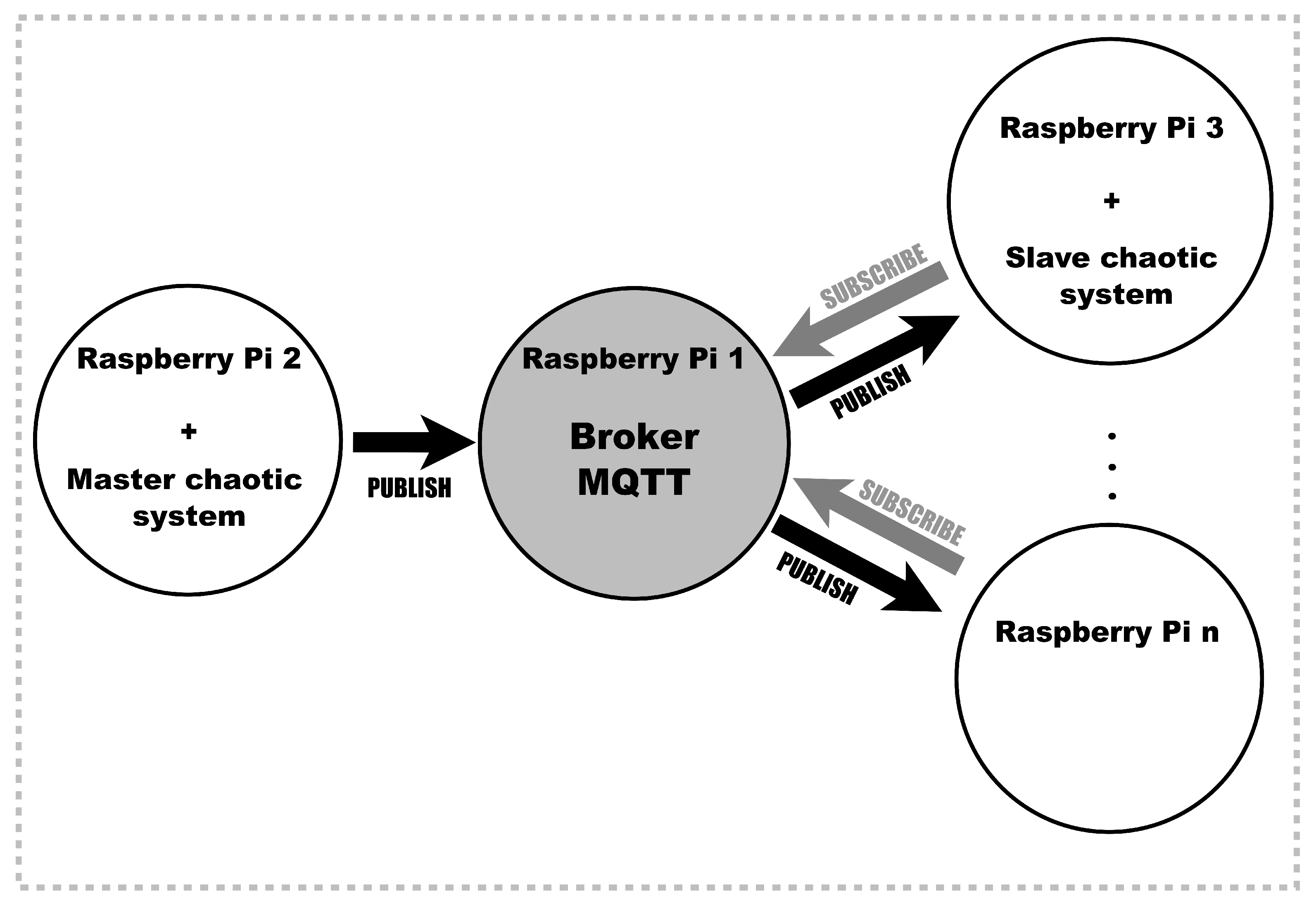
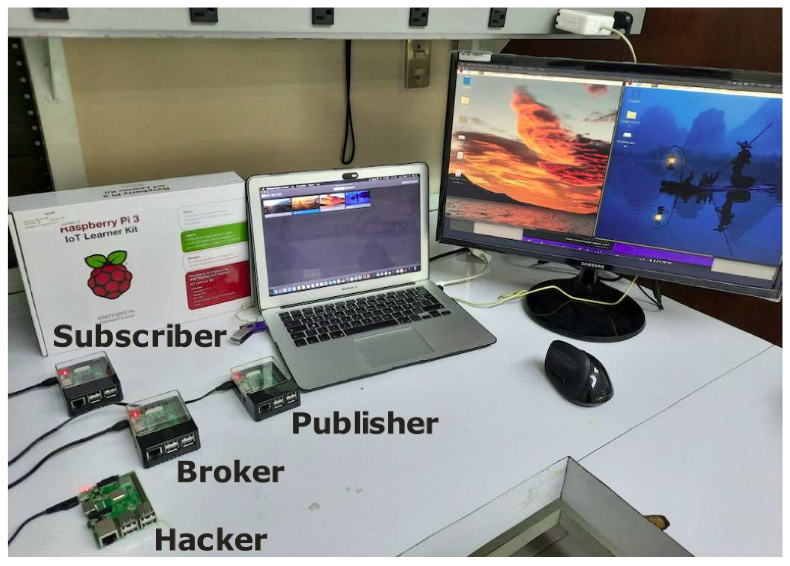
4. Hardware Implementation of an Image Encryption System on MQTT Based on Chaos

Once two chaotic systems are synchronized, they have the same behavior, and one can use the master system to encrypt an image that can be recovered by the slave. The channel can be wired or wireless, as performed herein by implementing the systems on MQTT for the IoT protocol. An intruder cannot recover the data because he or she must be synchronized with the transmitter and must have the same chaotic binary string, as detailed herein.

Figure 10 sketches the proposed system that is implemented on MQTT. The broker controls the communication among nodes that can become publishers (transmitter) or subscribers (receiver), but they have embedded a chaotic oscillator of different topologies, with different state variables, different parameters and different step sizes. This provides a preliminary key to perform private communication between a publisher and any number of subscribers. Another important thing is that the chaotic systems can have different initial conditions, and they synchronize as described in Section 3.

The systems sketched in Figure 10 can be programmed on RPis as shown in Figure 11. Raspberry Pi 2 is taken as the publisher that sends data to the broker (Raspberry Pi 1), which can be read by all subscribers (from Raspberry-Pi 3 to n). However, if the data are encrypted by a chaotic binary string, then the subscribers need to have the chaotic system to recover the original data. All subscribers can read the published data, but the synchronization between the publisher with any subscriber occurs by embedding the chaotic system and the synchronization method in the appropriate RPis. The chaotic binary strings are generated as detailed in [7].

The physical implementation of the secure transmission system is shown in Figure 12, where one can see four RPis labeled as publisher, broker, subscriber and hacker. The four RPis are monitored using the software “Microsoft Remote Desktop”, which visualizes the remote desks as shown in Figure 13. It works under the identification of the IP addresses of each RPi. The configuration window is shown in Figure 14, where the IP address of the RPi, denoted as “PC name”, the “User account” and the name of the node, which can be the same as the user account, can be appreciated. The other parameters can be left with the default values. One can visualize any number of nodes (RPis) connected under the MQTT protocol via Wi-Fi. The RPis can be in different local networks, and they can be connected through external servers that can be connected to the broker.

Before transmitting an image, the scheme in Figure 12 must be synchronized. This process is performed by publishing the values of the state variables at each iteration, which are provided by a numerical method, and the subscriber answers, sending the error between the read value and the one created by its embedded chaotic system. When the error is zero, the synchronization is successful as shown in Figure 15. Figure 15a shows the error when the publisher and subscriber are not synchronized (i.e., an intruder who does not embed the chaotic system must not have the opportunity to decrypt the data). Figure 15b shows the error when applying Hamiltonian forms and the observer approach, and Figure 15c shows the error when applying the OPCL method. The programming of the RPis was performed using Python and the 32-bit floating point format. The time taken to produce a synchronization error equal to 0 was 2.1 s on average when using 3B+ RPis, which include a wireless LAN 802.11 b/g/n of 2.4 GHz.

RGB images are encrypted by the random binary string generated by the Chen system in the publisher, as shown in Figure 12. The image is published in the broker, and after a subscriber synchronizes with the publisher, the image can be recovered. As the hacker does not synchronize, he or she cannot recover the image. Figure 16 and Figure 17 show the experimental results, in which one can see the original image, the image encrypted by the publisher, and the image recovered by the subscriber.

Table 4. Correlations between original and encrypted images (OEI) and between original and recovered images (ORI) transmitted using Raspberry Pis applying Hamiltonian forms and using Chen system.

Image	Correlation OEI	Correlation ORI
Lena 512 × 512 pixels	0.0066	1.0
Baboon 512 × 512 pixels	0.0109	1.0

shows the correlation analyses.

Other security tests were applied herein. The histogram analyses were performed according to [50] and are shown in Figure 18. For Lena, one can see that the Chen system was quite good for providing a uniform distribution to resist statistical attacks.

The key space was established by taking into account the initial conditions (${x_1}_0,{x_2}_0$ and ${x_3}_0$), parameters of the chaotic system ($a,b$ and c), and step size (h). By applying Hamiltonian forms, we added the gains ($k_{x1},k_{x2}$ and $k_{x3}$) so that all of them added up to 10 variables for the synchronized system, and since the implementation used 32-bit precision, it gave a key space of $2^{320}$. When applying the OPCL method, the gains k were replaced by the Hurwitz parameters ($p_1$ and $p_2$) so that 9 parameters existed, and the key space became $2^{288}$.

The correlation analysis for adjacent pixels (horizontal, vertical or diagonal) [51] is shown in

Table 5. Correlation coefficients (vertical, horizontal and diagonal) among adjacent pixels in original and encrypted Lena images using Chen system.

Correlation	Original Image	Encrypted Image
Vertical	0.9895	−0.0013
Horizontal	0.9796	0.0080
Diagonal	0.9689	−0.0113

for Lena (512 × 512 pixels). Figure 19 shows the distribution of the correlation of 10,000 pairs of adjacent pixels in vertical, horizontal and diagonal directions. As one can see, the adjacent pixels of the original image (left column) were highly correlated, but for the encrypted image (right column), the correlation changed, meaning that the dispersion was random.

The entropy analysis helped to appreciate the security of the cipher algorithm [52]. The Shanon H (s) entropy is defined by Equation (24), and the ideal value for a fully disordered image was eight. In this work, for the original Lena image (512 × 512 pixels), it was 7.27, and for the encrypted version using the Chen system, it was 7.9997. The entropy analyzed by colors yielded 7.9993, 7.9992 and 7.9992 for red, green and blue, respectively:

$$H\left(s\right)=\sum _{i=0}^{2^N-1}P\left(s_i\right)Lo{g}_2\left(\frac{1}{P\left(s_i\right)}\right)\mathrm{bit}.$$

(24)

Finally, we performed differential attack analyses, known as NPCR and UACI [53].

Table 6. NPCR and UACI analyses for encrypted Lena image (512 × 512 pixels).

Analysis	Color	Value (%)	Test with Critical Values [53]
NPCR	R	$99.5803$	successful
	G	$99.6246$	successful
	B	$99.5834$	successful
	RGB	$99.5961$	successful
UACI	R	$33.3723$	successful
	G	$33.4408$	successful
	B	$33.3834$	successful
	RGB	$33.3834$	successful

shows the results for the encrypted Lena image (512 × 512 pixels) using the Chen system. As one can see, all the critical values given in [53] were passed.

5. Conclusions

In this work, integer- and fractional-order chaotic systems were applied to encrypt color images that were transmitted under MQTT for the IoT protocol using Raspberry Pis, which were connected via Wi-Fi. The Chen system was the case study for generating random binary strings that were evaluated by the NIST and TestU01 tests. The best random sequence was obtained by performing post-processing with XOR. This random sequence was applied in the encryption process over MQTT, in which the publisher was synchronized with a subscriber by applying two synchronization methods, namely Hamiltonian forms and the OPCL method. In this manner, our proposed encryption method can be summarized as follows. The publisher sends an encrypted image that is only recovered by the subscriber that is embedding the same chaotic system; otherwise, the subscriber only reads noise-like data. This provides more privacy and security, and the average time for synchronization was measured to be 2.1 s over MQTT using Raspberry Pis over Wi-Fi. The encryption and decryption process for a color image such as Lena (512 × 512 pixels) took approximately 214 s. The proposed encryption/decryption system based on chaos under MQTT was tested by security and differential attack methods. All the tests—histogram, correlation among 10,000 pairs of adjacent pixels, entropy, NPCR and UACI,—were passed successfully, thus confirming the usefulness of chaotic systems in adding more security to MQTT for the transmission of encrypted images.

References

1. Lorenz, E.N. Deterministic nonperiodic flow. J. Atmos. Sci. 1963, 20, 130–141. [Google Scholar] [CrossRef] [Green Version]
2. Sira-Ramirez, H.; Cruz-Hernández, C. Synchronization of chaotic systems: A generalized Hamiltonian systems approach. Int. J. Bifurc. Chaos 2001, 11, 1381–1395. [Google Scholar] [CrossRef]
3. Li, X.; Zhou, L.; Tan, F. An image encryption scheme based on finite-time cluster synchronization of two-layer complex dynamic networks. Soft Comput. 2022, 26, 511–525. [Google Scholar] [CrossRef]
4. Yu, F.; Shen, H.; Zhang, Z.; Huang, Y.; Cai, S.; Du, S. A new multi-scroll Chua?s circuit with composite hyperbolic tangent-cubic nonlinearity: Complex dynamics, Hardware implementation and Image encryption application. Integration 2021, 81, 71–83. [Google Scholar] [CrossRef]
5. Deng, J.; Zhou, M.; Wang, C.; Wang, S.; Xu, C. Image segmentation encryption algorithm with chaotic sequence generation participated by cipher and multi-feedback loops. Multimed. Tools Appl. 2021, 80, 13821–13840. [Google Scholar] [CrossRef]
6. Gao, X.; Mou, J.; Xiong, L.; Sha, Y.; Yan, H.; Cao, Y. A fast and efficient multiple images encryption based on single-channel encryption and chaotic system. Nonlinear Dyn. 2022, 108, 613–636. [Google Scholar] [CrossRef]
7. Tlelo-Cuautle, E.; Pano-Azucena, A.D.; Guillén-Fernández, O.; Silva-Juárez, A. Analog/Digital Implementation of Fractional Order Chaotic Circuits and Applications; Springer: Berlin/Heidelberg, Germany, 2020. [Google Scholar]
8. Azizi, M.; Aickelin, U.; Khorshidi, H.A.; Shishehgarkhaneh, M.B. Shape and size optimization of truss structures by Chaos game optimization considering frequency constraints. J. Adv. Res. 2022. [Google Scholar] [CrossRef]
9. Hue, A.; Sharma, G.; Dricot, J.M. Privacy-Enhanced MQTT Protocol for Massive IoT. Electronics 2022, 11, 70. [Google Scholar] [CrossRef]
10. Liu, S.; Li, C.; Hu, Q. Cryptanalyzing Two Image Encryption Algorithms Based on a First-Order Time-Delay System. IEEE Multimed. 2022, 29, 74–84. [Google Scholar] [CrossRef]
11. Meshram, C.; Ibrahim, R.W.; Obaid, A.J.; Meshram, S.G.; Meshram, A.; El-Latif, A.M.A. Fractional chaotic maps based short signature scheme under human-centered IoT environments. J. Adv. Res. 2021, 32, 139–148. [Google Scholar] [CrossRef]
12. Radwan, A.; Moaddy, K.; Salama, K.; Momani, S.; Hashim, I. Control and switching synchronization of fractional order chaotic systems using active control technique. J. Adv. Res. 2014, 5, 125–132. [Google Scholar] [CrossRef] [Green Version]
13. Ahmad, I.; Ouannas, A.; Shafiq, M.; Pham, V.T.; Baleanu, D. Finite-time stabilization of a perturbed chaotic finance model. J. Adv. Res. 2021, 32, 1–14. [Google Scholar] [CrossRef] [PubMed]
14. Bertsias, P.; Psychalinos, C.; Maundy, B.J.; Elwakil, A.S.; Radwan, A.G. Partial fraction expansion-based realizations of fractional-order differentiators and integrators using active filters. Int. J. Circuit Theory Appl. 2019, 47, 513–531. [Google Scholar] [CrossRef]
15. Kapoulea, S.; Psychalinos, C.; Elwakil, A.S. Minimization of Spread of Time-Constants and Scaling Factors in Fractional-Order Differentiator and Integrator Realizations. Circuits Syst. Signal Process. 2018, 37, 5647–5663. [Google Scholar] [CrossRef]
16. Khanday, F.A.; Kant, N.A.; Dar, M.R.; Zulldfli, T.Z.A.; Psychalinos, C. Low-Voltage Low-Power Integrable CMOS Circuit Implementation of Integer- and Fractional-Order FitzHugh-Nagumo Neuron Model. IEEE Trans. Neural Netw. Learn. Syst. 2019, 30, 2108–2122. [Google Scholar] [CrossRef] [PubMed]
17. Sanchez-Sinencio, E.; Geiger, R.L.; Nevarez-Lozano, H. Generation of continuous-time two integrator loop OTA filter structures. IEEE Trans. Circuits Syst. 1988, 35, 936–946. [Google Scholar] [CrossRef]
18. Sprott, J.C. Some simple chaotic flows. Phys. Rev. E 1994, 50, R647. [Google Scholar] [CrossRef] [PubMed]
19. Schuster, H.G.; Just, W. Deterministic Chaos: An Introduction; John Wiley & Sons: Hoboken, NJ, USA, 2006. [Google Scholar]
20. Parker, T.S.; Chua, L. Practical Numerical Algorithms for Chaotic Systems; Springer Science & Business Media: Berlin/Heidelberg, Germany, 2012. [Google Scholar]
21. Wolf, A.; Swift, J.B.; Swinney, H.L.; Vastano, J.A. Determining Lyapunov exponents from a time series. Phys. D Nonlinear Phenom. 1985, 16, 285–317. [Google Scholar] [CrossRef] [Green Version]
22. Hegger, R.; Kantz, H.; Schreiber, T. Practical implementation of nonlinear time series methods: The TISEAN package. Chaos Interdiscip. J. Nonlinear Sci. 1999, 9, 413–435. [Google Scholar] [CrossRef] [Green Version]
23. Tlelo-Cuautle, E.; De La Fraga, L.G.; Guillén-Fernández, O.; Silva-Juárez, A. Optimization of Integer/Fractional Order Chaotic Systems by Metaheuristics and Their Electronic Realization; CRC Press: Boca Raton, FL, USA, 2021. [Google Scholar]
24. Hooker, J.N. Testing heuristics: We have it all wrong. J. Heuristics 1995, 1, 33–42. [Google Scholar] [CrossRef]
25. Coello, C.A.C. A comprehensive survey of evolutionary-based multiobjective optimization techniques. Knowl. Inf. Syst. 1999, 1, 269–308. [Google Scholar] [CrossRef]
26. Rosenberg, R.S. Stimulation of genetic populations with biochemical properties: I. the model. Math. Biosci. 1970, 7, 223–257. [Google Scholar] [CrossRef]
27. Deb, K.; Agrawal, S.; Pratap, A.; Meyarivan, T. A fast elitist non-dominated sorting genetic algorithm for multi-objective optimization: NSGA-II. In Proceedings of the International Conference on Parallel Problem Solving from Nature, Paris, France, 18–20 September 2000; pp. 849–858. [Google Scholar]
28. Abarbanel, H.D.; Brown, R.; Sidorowich, J.J.; Tsimring, L.S. The analysis of observed chaotic data in physical systems. Rev. Mod. Phys. 1993, 65, 1331. [Google Scholar] [CrossRef] [Green Version]
29. Yalçin, M.E. Increasing the entropy of a random number generator using n-scroll chaotic attractors. Int. J. Bifurc. Chaos 2007, 17, 4471–4479. [Google Scholar] [CrossRef]
30. Rukhin, A.; Soto, J.; Nechvatal, J.; Smid, M.; Barker, E. A Statistical Test Suite for Random and Pseudorandom Number Generators for Cryptographic Applications; Technical Report; Booz-Allen and Hamilton Inc.: Mclean, VA, USA, 2001. [Google Scholar]
31. L’ecuyer, P.; Simard, R. TestU01: AC library for empirical testing of random number generators. ACM Trans. Math. Softw. (TOMS) 2007, 33, 1–40. [Google Scholar] [CrossRef]
32. Pareschi, F.; Rovatti, R.; Setti, G. Simple and effective post-processing stage for random stream generated by a chaos-based RNG. In Proceedings of the NOLTA, Bologna, Italy, 11–14 September 2006; pp. 383–386. [Google Scholar]
33. Boccaletti, S.; Kurths, J.; Osipov, G.; Valladares, D.; Zhou, C. The synchronization of chaotic systems. Phys. Rep. 2002, 366, 1–101. [Google Scholar] [CrossRef]
34. Pecora, L.M.; Carroll, T.L. Synchronization in chaotic systems. Phys. Rev. Lett. 1990, 64, 821. [Google Scholar] [CrossRef]
35. Carroll, T.L.; Pecora, L.M. Synchronizing chaotic circuits. IEEE Trans. Circuits Syst. 1991, 38, 453–456. [Google Scholar] [CrossRef] [Green Version]
36. Lerescu, A.; Constandache, N.; Oancea, S.; Grosu, I. Collection of master—Slave synchronized chaotic systems. Chaos Solitons Fractals 2004, 22, 599–604. [Google Scholar] [CrossRef] [Green Version]
37. Melendez-Cano, A.; Rodriguez, J.S.; Sandoval-Ibarra, Y.; Cardenas-Valdez, J.R.; Garcia-Ortega, M.J.; Tlelo-Cuautle, E.; Nuñez-Perez, J.C. Chaotic Synchronization of Sprott Collection and RGB Image Transmission. In Proceedings of the Mechatronics, Electronics and Automotive Engineering (ICMEAE), 2017 International Conference, Cuernavaca, Mexico, 21–24 November 2017; pp. 49–54. [Google Scholar]
38. Vaidyanathan, S.; Sampath, S.; Azar, A.T. Global chaos synchronisation of identical chaotic systems via novel sliding mode control method and its application to Zhu system. Int. J. Model. Identif. Control. 2015, 23, 92–100. [Google Scholar] [CrossRef]
39. Chen, X.; Park, J.H.; Cao, J.; Qiu, J. Sliding mode synchronization of multiple chaotic systems with uncertainties and disturbances. Appl. Math. Comput. 2017, 308, 161–173. [Google Scholar] [CrossRef]
40. Rajagopal, K.; Karthikeyan, A.; Srinivasan, A.K. FPGA implementation of novel fractional-order chaotic systems with two equilibriums and no equilibrium and its adaptive sliding mode synchronization. Nonlinear Dyn. 2017, 87, 2281–2304. [Google Scholar] [CrossRef]
41. Nosrati, K.; Volos, C.; Azemi, A. Cubature Kalman filter-based chaotic synchronization and image encryption. Signal Process. Image Commun. 2017, 58, 35–48. [Google Scholar] [CrossRef]
42. Abd, M.H.; Tahir, F.R.; Al-Suhail, G.A.; Pham, V.T. An adaptive observer synchronization using chaotic time-delay system for secure communication. Nonlinear Dyn. 2017, 90, 2583–2598. [Google Scholar] [CrossRef]
43. Wang, Y.; Karimi, H.R.; Yan, H. An adaptive event-triggered synchronization approach for chaotic Lur?e systems subject to aperiodic sampled data. IEEE Trans. Circuits Syst. II Express Briefs 2018, 66, 442–446. [Google Scholar] [CrossRef]
44. Vaidyanathan, S.; Volos, C.; Pham, V.T.; Madhavan, K. Analysis, adaptive control and synchronization of a novel 4-D hyperchaotic hyperjerk system and its SPICE implementation. Arch. Control. Sci. 2015, 25, 135–158. [Google Scholar] [CrossRef]
45. Vaidyanathan, S.; Akgul, A.; Kaçar, S.; Çavuşoğlu, U. A new 4-D chaotic hyperjerk system, its synchronization, circuit design and applications in RNG, image encryption and chaos-based steganography. Eur. Phys. J. Plus 2018, 133, 46. [Google Scholar] [CrossRef]
46. Pham, V.T.; Kingni, S.T.; Volos, C.; Jafari, S.; Kapitaniak, T. A simple three-dimensional fractional-order chaotic system without equilibrium: Dynamics, circuitry implementation, chaos control and synchronization. AEU-Int. J. Electron. Commun. 2017, 78, 220–227. [Google Scholar] [CrossRef]
47. Daltzis, P.A.; Volos, C.K.; Nistazakis, H.E.; Tsigopoulos, A.D.; Tombras, G.S. Analysis, Synchronization and Circuit Design of a 4D Hyperchaotic Hyperjerk System. Computation 2018, 6, 14. [Google Scholar] [CrossRef] [Green Version]
48. Ye, G.; Pan, C.; Huang, X.; Zhao, Z.; He, J. A Chaotic Image Encryption Algorithm Based on Information Entropy. Int. J. Bifurc. Chaos 2018, 28, 1850010. [Google Scholar] [CrossRef]
49. Jackson, E.A.; Grosu, I. An open-plus-closed-loop (OPCL) control of complex dynamic systems. Phys. D Nonlinear Phenom. 1995, 85, 1–9. [Google Scholar] [CrossRef]
50. Zhou, S.; Wang, X.; Wang, M.; Zhang, Y. Simple colour image cryptosystem with very high level of security. Chaos Solitons Fractals 2020, 141, 110225. [Google Scholar] [CrossRef]
51. Yousif, S.F.; Abboud, A.J.; Radhi, H.Y. Robust image encryption with scanning technology, the El-Gamal algorithm and chaos theory. IEEE Access 2020, 8, 155184–155209. [Google Scholar] [CrossRef]
52. Flores-Vergara, A.; García-Guerrero, E.; Inzunza-González, E.; López-Bonilla, O.; Rodríguez-Orozco, E.; Cárdenas-Valdez, J.; Tlelo-Cuautle, E. Implementing a chaotic cryptosystem in a 64-bit embedded system by using multiple-precision arithmetic. Nonlinear Dyn. 2019, 96, 497–516. [Google Scholar] [CrossRef]
53. Wu, Y.; Noonan, J.P.; Agaian, S. NPCR and UACI randomness tests for image encryption. Cyber J. Multidiscip. J. Sci. Technol. J. Sel. Areas Telecommun. (JSAT) 2011, 1, 31–38. [Google Scholar]
Figure 1. Pareto front after optimizing LE+ and D K Y of the Chen system in Equation (1) when applying NSGA-II.
Mathematics 10 01907 g001
Figure 2. Chaotic attractors of the Chen system in Equation (1) using the parameters of the: (a) first row, (b) second row, (c) third row, (d) fourth row, (e) fifth row, and (f) sixth row, given in Table 1.
Mathematics 10 01907 g002
Figure 3. (a) Autocorrelation of the chaotic time series x 1 of the Chen system. (b) Detail of the correlation with the first zero crossing.
Mathematics 10 01907 g003
Figure 4. Portraits of the master–slave variables of Equation (2) synchronized by Hamiltonian forms and by setting a = 39.260116 , b = 3.2218111 and c = 29.760754 , and k 1 = k 2 = k 3 = 10 : (a) x 1 , (b) x 2 and (c) x 3 .
Mathematics 10 01907 g004
Figure 5. Time series of the master–slave systems of Equation (2) synchronized by Hamiltonian forms, as shown in Figure 4.
Mathematics 10 01907 g005
Figure 6. Synchronization errors from Figure 4 and Figure 5, applying Hamiltonian forms and the observer approach.
Mathematics 10 01907 g006
Figure 7. Portraits of the master–slave variables synchronized by OPCL: (a) x 1 , (b) x 2 and (c) x 3 , setting a = 39.260116 , b = 3.2218111 and c = 29.760754 with P 1 = 33 .
Mathematics 10 01907 g007
Figure 8. Times series of the master–slave systems synchronized by OPCL, as shown in Figure 7.
Mathematics 10 01907 g008
Figure 9. Synchronization errors from Figure 7 and Figure 8 when applying the OPCL method.
Mathematics 10 01907 g009
Figure 10. MQTT protocol using chaotic systems in the nodes controlled by a broker for image encryption.
Mathematics 10 01907 g010
Figure 11. Secure transmission of data on MQTT protocol using Raspberry Pis synchronized by chaotic systems, which are embedded as sketched in Figure 10.
Mathematics 10 01907 g011
Figure 12. Physical realization of the secure communication system on MQTT for IoT protocol using RPis.
Mathematics 10 01907 g012
Figure 13. Remote desktops of the RPis shown in Figure 12.
Mathematics 10 01907 g013
Figure 14. Configuration of software “Microsoft Remote Desktop”.
Mathematics 10 01907 g014
Figure 15. Synchronization errors in Figure 12 programmed in Python when the publisher and subscriber (a) never synchronize (hacker case), (b) synchronize with Hamiltonian forms and (c) synchronize with OPCL method.
Mathematics 10 01907 g015
Figure 16. Encrypting Lena: (a) original Image, (b) encrypted image and (c) recovered image.
Mathematics 10 01907 g016
Figure 17. Encrypting Baboon: (a) original image, (b) encrypted image and (c) recovered image.
Mathematics 10 01907 g017
Figure 18. Histograms of Lena: (a) original image (red color), (b) encrypted image of R, (c) original image (green color), (d) encrypted image of G, (e) original image (blue color) and (f) encrypted image of B.
Mathematics 10 01907 g018
Figure 19. Correlation of adjacent pixels for Lena (512 × 512 pixels). The left column shows (a) vertical, (c) horizontal and (e) diagonal directions of the original image, and the right column shows (b) vertical, (d) horizontal and (f) diagonal directions of the encrypted image using the Chen system.
Mathematics 10 01907 g019