Quantum Weighted Fractional Fourier Transform

Abstract

Quantum Fourier transform (QFT) is an important part of many quantum algorithms. However, there are few reports on quantum fractional Fourier transform (QFRFT). The main reason is that the definitions of fractional Fourier transform (FRFT) are diverse, while some definitions do not include unitarity, which leads to some studies pointing out that there is no QFRFT. In this paper, we first present a reformulation of the weighted fractional Fourier transform (WFRFT) and prove its unitarity, thereby proposing a quantum weighted fractional Fourier transform (QWFRFT). The proposal of QWFRFT provides the possibility for many quantum implementations of signal processing.

1. Introduction

Feynman was the first to present the idea of quantum computing, that is, to directly use the state of microscopic particles to represent quantum information, which is considered to be the early prototype of the concept of quantum computing [1]. Subsequently, Deutsch formalized the concept of quantum computing, proposed the idea of a quantum Turing machine, and designed the first quantum parallel algorithm, which exhibited excellent performance beyond classical computing [2]. The proposal of Shor’s algorithm caused researchers to realize that quantum computing had a natural parallel processing capability, which could introduce many disruptive technological innovations. Shor’s algorithm states that a large number can be decomposed into the product of two prime factors in polynomial time. This greatly challenged the RSA (Rivest–Shamir–Adleman) encryption system, thus indicating that the RSA encryption system had been cracked in theory [3,4]. Grover’s search algorithm convinced researchers of the power of quantum computing. Compared with the traditional search method, this algorithm can achieve the acceleration effect of square level [5]. Therefore, many improved Grover search algorithms have been proposed [6,7,8,9,10]. Meanwhile, quantum-inspired algorithms have also been proposed that can be simulated by classical computing [11,12,13,14,15,16]. Moreover, the quantum algorithm has been applied to solve linear systems of equations, which introduced new ideas for solving linear equations. This algorithm is also called the HHL algorithm [17]. The HHL algorithm has been widely used, and its improved algorithms have been continuously proposed [18,19,20]. Recently, quantum algorithms have been applied to solve differential equations [21,22,23,24]. A series of quantum computing technologies, such as quantum Fourier transform [25], quantum phase estimation [26], and the HHL algorithm, are called quantum basic linear algebra assembly [27]. At present, quantum computing has been widely used in cryptography, quantum simulation, machine learning, and other fields and shows a strong ability and great potential.

The Fourier transform plays an important role in the design of quantum algorithms, but little is known about the quantum algorithms of the fractional Fourier transform (FRFT). The initial definition of the FRFT was proposed in [28]. Its application provides a convenient technique for solving certain classes of ordinary and partial differential equations, which arise in quantum mechanics from classical quadratic Hamiltonians. The theoretical research of the FRFT has developed rapidly, and various definitions have been proposed, such as eigenvalue FRFT [29], weighted FRFT [30], and sampling FRFT [31]. These definitions are widely used in various fields of signal processing. So far, little is known about the reports and studies on the quantum fractional Fourier transform (QFRFT). The main reason is that the design of quantum algorithms should satisfy unitarity, and some FRFTs do not include unitarity. Thus, a quantum pseudo-fractional Fourier transform (QPFRFT) was proposed [32], and the authors showed that there was no QFRFT. However, we present a reformulation of the weighted fractional Fourier transform (WFRFT) and prove its unitarity, whereupon a quantum weighted fractional Fourier transform (QWFRFT) is proposed.

The remainder of this paper is organized as follows. The preliminary knowledge is described in Section 2. The unitarity of the WFRFT is proved in Section 3. Section 4 presents the QWFRFT. Finally, the conclusions are presented in Section 5.

2. Preparation

For a unitary matrix $U$, assuming that it has an eigenvector $|u\rangle$ and the corresponding eigenvalue $e^{2\pi i\phi }$, $U|u\rangle =e^{2\pi i\phi }|u\rangle$ is satisfied. Therefore, we can calculate $\phi$ through the phase estimation algorithm. The circuit of phase estimation is shown in Figure 1. It is not difficult to find that the quantum Fourier transform (QFT) is the key to phase estimation, and phase estimation is the key of many quantum algorithms.

The importance of the QFT goes without saying. However, little is known about the report of the QFRFT. In 2012, Parasa et al. proposed a QPFRFT using multiple-valued logic [32]. The reason why researchers call it “pseudo” is that the FRFT used did not include unitarity. The FRFT was proposed by Bailey et al. [33], and its definition is as follows:

$$F^{\alpha }\left[k\right]={\displaystyle \sum _{j=0}^{N-1}f\left[j\right]·\exp \left(2\pi i·\frac{kj}{N}·\alpha \right)}.$$

(1)

Parasa et al. pointed out: “It must be noted that unlike the discrete Fourier transform, the FRFT is not a unitary operation. More formally, this means that there exists no unitary operator which can implement the following quantum computational operation”.

$${\displaystyle \sum _{j=0}^{N-1}f\left(j\right)|j\rangle }\stackrel{NOTPOSSLBLE}{\to }{\displaystyle \sum _{k=0}^{N-1}{F}^{\alpha }\left(k\right)|k\rangle }.$$

(2)

Therefore, Parasa et al. explicitly state that it is not possible to define the QFRFT. However, the definitions of the FRFT are diverse, and the definition of one class of WFRFT includes unitarity. Hence, Parasa et al.’s statement that there is no QFRFT is not rigorous.

In 1995, Shih proposed the definition of a WFRFT [30]. The alpha-order FRFT of the function $f\left(t\right)$ can be expressed as

$$F^{\alpha }\left[f\left(t\right)\right]={\displaystyle \sum _{l=0}^3{A}_l\left(\alpha \right)f_l\left(t\right)}.$$

(3)

Here,$f_0\left(t\right)=f\left(t\right)$, $f_1(t)=F\left[f_0\left(t\right)\right]$, $f_2\left(t\right)=F\left[f_1\left(t\right)\right]$, and $f_3\left(t\right)=F\left[f_2\left(t\right)\right]$ (F denotes Fourier transform). The weighting coefficient $A_l(\alpha )$ is expressed as

$$A_l(\alpha )=\cos \left(\frac{(\alpha -l)\pi }{4}\right)\cos \left(\frac{2(\alpha -l)\pi }{4}\right)\exp \left(\frac{3(\alpha -l)i\pi }{4}\right),$$

(4)

where $l=0,1,2,3$.

3. Unitarity of Weighted Fractional Fourier Transform

A complex matrix $U$ satisfies

$${UU}^H=U^{H}U=I,$$

(5)

where $H$ denotes the conjugate transpose, and I is the identity matrix. Then, matrix $U$ is called a unitary matrix.

The discrete form of the WFRFT (Equation (3)) can be expressed as

$$DWFRFT=A_0\left(\alpha \right)·I+A_1\left(\alpha \right)·DFT+A_2\left(\alpha \right)·{DFT}^2+A_3\left(\alpha \right)·{DFT}^3,$$

(6)

where $A_l\left(\alpha \right)$ is Equation (4), and $DFT$ is the discrete Fourier transform. It is not easy to prove the unitarity of Equation (6). Therefore, we present the reformulation of the WFRFT and prove its unitarity. First, Equation (4) can be written as

$$\begin{array}{cc}\hfill A_l(\alpha )& =\cos \left(\frac{(\alpha -l)\pi }{4}\right)\cos \left(\frac{2(\alpha -l)\pi }{4}\right)\exp \left(\frac{3(\alpha -l)i\pi }{4}\right)\hfill \\ & =\frac{1}{2}\times \left[\exp \left(\frac{(\alpha -l)\pi i}{4}\right)+\exp \left(\frac{-(\alpha -l)\pi i}{4}\right)\right]\hfill \\ & \times \frac{1}{2}\times \left[\exp \left(\frac{2(\alpha -l)\pi i}{4}\right)+\exp \left(\frac{-2(\alpha -l)\pi i}{4}\right)\right]\times \exp \left(\frac{3(\alpha -l)i\pi }{4}\right)\hfill \\ & =\frac{1}{4}\left(1+\exp \left(\frac{2(\alpha -l)\pi i}{4}\right)+\exp \left(\frac{4(\alpha -l)\pi i}{4}\right)+\exp \left(\frac{6(\alpha -l)\pi i}{4}\right)\right)\hfill \\ & =\frac{1}{4}{\displaystyle \sum _{k=0}^3\exp \left(\frac{2\pi i}{4}(\alpha -l)k\right)}\hfill \\ & =\frac{1}{4}{\displaystyle \sum _{k=0}^3\exp \left(\frac{2\pi i\alpha k}{4}\right)}\exp \left(\frac{-2\pi ilk}{4}\right).\hfill \end{array}$$

(7)

Let $B_k^{\alpha }=\exp \left(\frac{2\pi ik\alpha }{4}\right)$; $k=0,1,2,3$; then, Equation (7) can be expressed as

$$\left(\begin{array}{l}{A}_0^{\alpha }\\ A_1^{\alpha }\\ A_2^{\alpha }\\ A_3^{\alpha }\end{array}\right)=\frac{1}{4}\left(\begin{array}{cccc}1& 1& 1& 1\\ 1& -i& -1& i\\ 1& -1& 1& -1\\ 1& i& -1& -i\end{array}\right)\left(\begin{array}{l}{B}_0^{\alpha }\\ B_1^{\alpha }\\ B_2^{\alpha }\\ B_3^{\alpha }\end{array}\right).$$

(8)

We write Equation (6) as Equation (9).

$$DWFRFT=\left(I,DFT,{DFT}^2,{DFT}^3\right)\left(\begin{array}{c}{A}_0\left(\alpha \right)\\ A_1\left(\alpha \right)\\ A_2\left(\alpha \right)\\ A_3\left(\alpha \right)\end{array}\right).$$

(9)

Equation (8) is substituted into Equation (9), and we obtain

$$DWFRFT=\frac{1}{4}\left(I,DFT,{DFT}^2,{DFT}^3\right)\left(\begin{array}{cccc}1& 1& 1& 1\\ 1& -i& -1& i\\ 1& -1& 1& -1\\ 1& i& -1& -i\end{array}\right)\left(\begin{array}{l}{B}_0^{\alpha }\\ B_1^{\alpha }\\ B_2^{\alpha }\\ B_3^{\alpha }\end{array}\right).$$

(10)

We let

$$\{\begin{array}{l}{Y}_0=I+DFT+{DFT}^2+{DFT}^3\\ Y_1=I-i·DFT-{DFT}^2+i·{DFT}^3\\ Y_2=I-DFT+{DFT}^2-{DFT}^3\\ Y_3=I+i·DFT-{DFT}^2-i·{DFT}^3\end{array}$$

(11)

Definition 1.

A reformulation of the DWFRFT.

$$\begin{array}{ccc}\hfill DWFRFT& =& \frac{1}{4}\left(Y_0,Y_1,Y_2,Y_3\right)\left(\begin{array}{l}{B}_0^{\alpha }\\ B_1^{\alpha }\\ B_2^{\alpha }\\ B_3^{\alpha }\end{array}\right)\hfill \\ & =& \frac{1}{4}\left(Y_0{B}_0^{\alpha }+Y_1{B}_1^{\alpha }+Y_2{B}_2^{\alpha }+Y_3{B}_3^{\alpha }\right)\hfill \\ & =& \frac{1}{4}{\displaystyle \sum _{k=0}^3{Y}_k{B}_k^{\alpha }}.\hfill \end{array}$$

(12)

where$B_k^{\alpha }=\exp \left(\frac{2\pi ik\alpha }{4}\right)$; $k=0,1,2,3$.

Proposition 1.

$Y_k$are real symmetric matrices.

Proof of Proposition 1.

In Equation (11), I is the identity matrix, and $DFT$ can be expressed as

$$DFT=\frac{1}{\sqrt{N}}·\left(\begin{array}{cccc}{u}^{0\times 0}& u^{0\times 1}& \dots & u^{0\times (n-1)}\\ u^{1\times 0}& u^{1\times 1}& \dots & u^{1\times (n-1)}\\ ⋮& ⋮& \ddots & ⋮\\ u^{(n-1)\times 0}& u^{(n-1)\times 1}& \dots & u^{(n-1)\times (n-1)}\end{array}\right),$$

(13)

where $u=\exp \left(-2\pi i/N\right)$. Here, $DFT$ is a symmetric matrix, so that ${DFT}^2$, ${DFT}^3$, and ${DFT}^4$ are also symmetric matrices. We know that the result of adding symmetric matrices is still a symmetric matrix. Therefore, $Y_k$ are symmetric matrices (Equation (11)).

Next, we prove that $Y_k$ are real matrices. The integer powers of the Fourier transform are shown in Figure 2. Here, ${DFT}^2$ and ${DFT}^4$ are real matrices; the matrix of ${DFT}^2$ is shown in Equation (14), and ${DFT}^4$ is the identity matrix ${DFT}^4=DF{T}^0=I$.

$${DFT}^2=\left(\begin{array}{cccc}1& 0& \dots & 0\\ 0& 0& \dots & 1\\ ⋮& ⋮& ⋰& ⋮\\ 0& 1& \dots & 0\end{array}\right).$$

(14)

Obviously, $I$ and ${DFT}^2$ are real matrices. In Equation (13), each element of the $DFT$ can be expressed as

$$u_{lk}=\exp \left(-2\pi ilk/N\right),$$

(15)

where $l=0,1,\dots ,n-1$;$k=0,1,\dots ,n-1$. Therefore, ${DFT}^3$ is an inverse Fourier transform, and each element of its matrix can be expressed as

$$w_{lk}=\exp \left(2\pi ilk/N\right),$$

(16)

where $l=0,1,\dots ,n-1$; $k=0,1,\dots ,n-1$. Thus, the result of $DFT+{DFT}^3$ is a real number,

$$\begin{array}{cc}\hfill w_{lk}+u_{lk}& =\exp \left(-2\pi ilk/N\right)+\exp \left(2\pi ilk/N\right)\hfill \\ & =\cos \left(2\pi lk/N\right)-i\sin \left(2\pi lk/N\right)+\cos \left(2\pi lk/N\right)+i\sin \left(2\pi lk/N\right)\hfill \\ & =2\cos \left(2\pi lk/N\right).\hfill \end{array}$$

(17)

The result for $-iDFT+{iDFT}^3$ is

$$\begin{array}{cc}\hfill -i{w}_{lk}+i{u}_{lk}& =-i\exp \left(-2\pi ilk/N\right)+i\exp \left(2\pi ilk/N\right)\hfill \\ & =-i\cos \left(2\pi lk/N\right)-\sin \left(2\pi lk/N\right)+i\cos \left(2\pi lk/N\right)-\sin \left(2\pi lk/N\right)\hfill \\ & =-2\sin \left(2\pi lk/N\right).\hfill \end{array}$$

(18)

The result for $-DFT-{DFT}^3$ is

$$\begin{array}{cc}\hfill -w_{lk}-u_{lk}& =-\exp \left(-2\pi ilk/N\right)-\exp \left(2\pi ilk/N\right)\hfill \\ & =-\cos \left(2\pi lk/N\right)+i\sin \left(2\pi lk/N\right)-\cos \left(2\pi lk/N\right)-i\sin \left(2\pi lk/N\right)\hfill \\ & =-2\cos \left(2\pi lk/N\right).\hfill \end{array}$$

(19)

The result for $iDFT-{iDFT}^3$ is

$$\begin{array}{cc}\hfill i{w}_{lk}-i{u}_{lk}& =i\exp \left(-2\pi ilk/N\right)-i\exp \left(2\pi ilk/N\right)\hfill \\ & =i\cos \left(2\pi lk/N\right)+\sin \left(2\pi lk/N\right)-i\cos \left(2\pi lk/N\right)+\sin \left(2\pi lk/N\right)\hfill \\ & =2\sin \left(2\pi lk/N\right).\hfill \end{array}$$

(20)

Therefore, for Equation (11), $Y_k$ are real symmetric matrices. □

Proposition 2.

The weighted fractional Fourier transform is unitary.

Proof of Proposition 2.

By the proof of Proposition 1, we know that $Y_k$ are real symmetric matrices; that is, ${\left(Y_k\right)}^H=Y_k$. Therefore, the conjugate transpose of the DWFRFT is

$$\begin{array}{ccc}\hfill {\left(DWFRFT\right)}^H& =& \frac{1}{4}{\left(Y_0{B}_0^{\alpha }+Y_1{B}_1^{\alpha }+Y_2{B}_2^{\alpha }+Y_3{B}_3^{\alpha }\right)}^H\hfill \\ & =& \frac{1}{4}\left(Y_0{B}_0^{-\alpha }+Y_1{B}_1^{-\alpha }+Y_2{B}_2^{-\alpha }+Y_3{B}_3^{-\alpha }\right).\hfill \end{array}$$

(21)

Thus, we obtain

$$\begin{array}{ccc}\hfill DWFRFT·{\left(DWFRFT\right)}^H& =& \frac{1}{16}\left(Y_0{B}_0^{\alpha }+Y_1{B}_1^{\alpha }+Y_2{B}_2^{\alpha }+Y_3{B}_3^{\alpha }\right)\left(Y_0{B}_0^{-\alpha }+Y_1{B}_1^{-\alpha }+Y_2{B}_2^{-\alpha }+Y_3{B}_3^{-\alpha }\right)\hfill \\ & =& \frac{1}{16}{\displaystyle \sum _{k=0}^3{\displaystyle \sum _{l=0}^3{Y}_k{Y}_l{B}_k^{\alpha }{B}_l^{-\alpha }}}.\hfill \end{array}$$

(22)

Here,

$$Y_k{Y}_l=\{\begin{array}{l}0,k\ne l\\ Y_k^2,k=l\end{array}$$

(23)

Then, Equation (22) is written as

$$DWFRFT·{\left(DWFRFT\right)}^H=\frac{1}{16}{\displaystyle \sum _{k=0}^3{Y}_k^2}.$$

(24)

After calculation, we know that $Y_k^2=4Y_k$. Equation (25) is obtained.

$$DWFRFT·{\left(DWFRFT\right)}^H=\frac{1}{4}{\displaystyle \sum _{k=0}^3{Y}_k}=\frac{1}{4}\left(Y_0+Y_1+Y_2+Y_3\right)=I.$$

(25)

Thus, the unitarity of the WFRFT is proved. □

We can also implement the new reformulation with the help of fast Fourier transform (FFT), and its implementation module is shown in Figure 3. The weighting coefficients are readjusted $A_l^{\alpha }$ in Figure 3; so, the computational complexity is $O\left(N\log N\right)$.

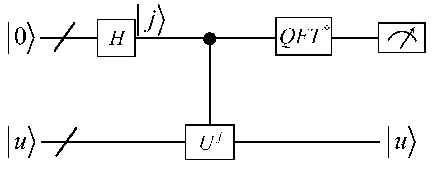
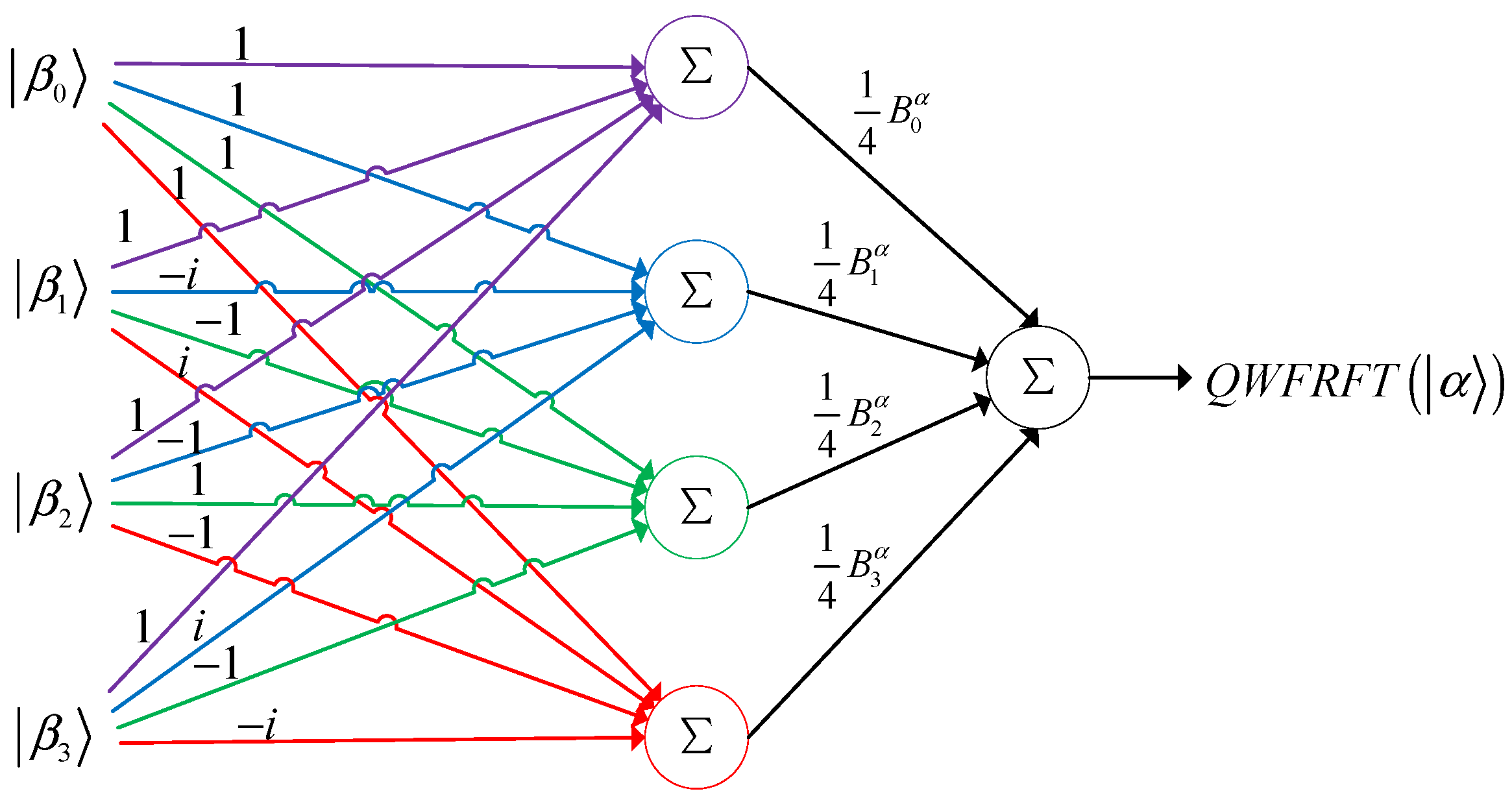
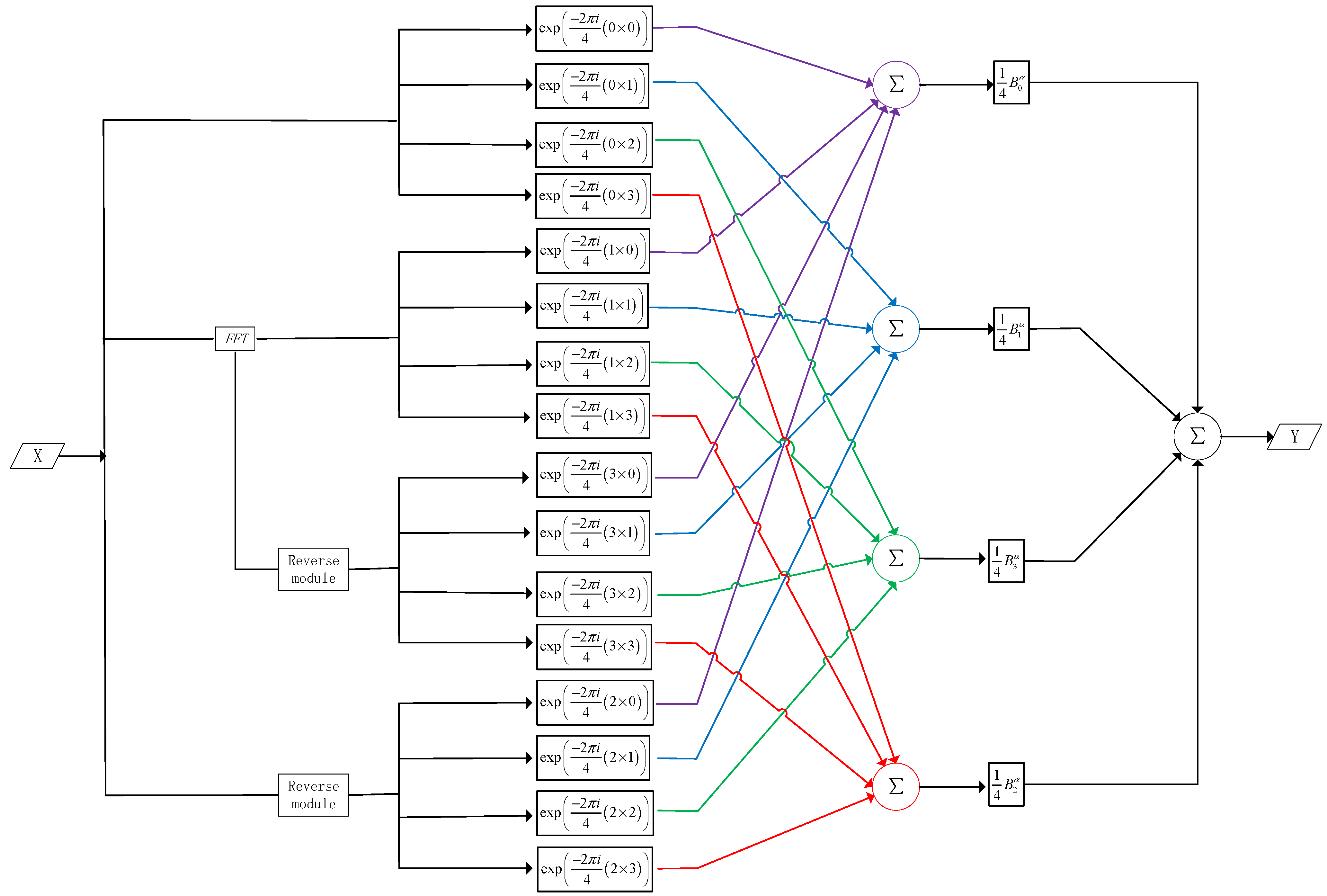
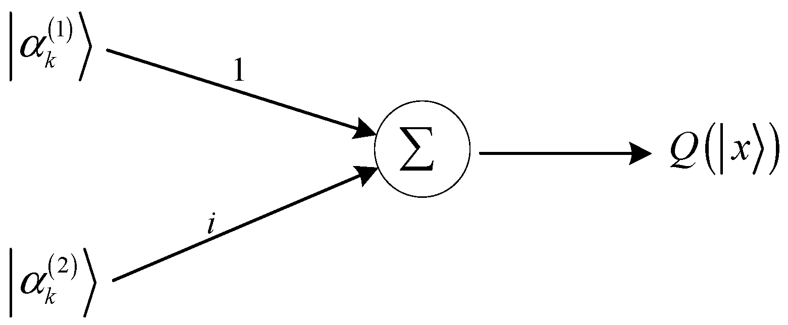
4. Quantum Weighted Fractional Fourier Transform

In this section, we will present the QWFRFT with the help of the QFT. The QFT is an application of the classical Fourier transform to the amplitude of a quantum state. the vector x is transformed into the vector y by the classical Fourier transform,

$$y_k=\frac{1}{\sqrt{N}}{\displaystyle \sum _{j=0}^{N-1}{x}_j{u}^{jk}};k=0,1,2,\dots ,N-1$$

(26)

where $u=e^{-2\pi i/N}$ and $N$ is the signal length.

Similarly, QFT is applied to quantum state $|x\rangle ={\displaystyle \sum _{j=0}^{N-1}{x}_j|j\rangle }$ to obtain quantum state $|y\rangle ={\displaystyle \sum _{k=0}^{N-1}{y}_k|k\rangle }$, and we have

$$y_k=\frac{1}{\sqrt{N}}{\displaystyle \sum _{j=0}^{N-1}{x}_j{w}_n^{jk}},$$

(27)

where $k=0,1,2,\dots ,N-1$ and $w=e^{2\pi i/N}$. We note that Equation (27) is the inverse of the classical discrete Fourier transform; by convention, the QFT has the same effect as the inverse discrete Fourier transform.

In case that $|j\rangle$ is a basis state, the QFT can also be expressed as the map

$$QFT:|j\rangle \mapsto \frac{1}{\sqrt{N}}{\displaystyle \sum _{k=0}^{N-1}{w}^{jk}|k\rangle }.$$

(28)

Equivalently, the QFT can be viewed as a unitary matrix acting on quantum state vectors, where the unitary matrix $F_N$ is given by

$$F_N=\frac{1}{\sqrt{N}}\left(\begin{array}{cccc}{w}^{0\times 0}& w^{0\times 1}& \dots & w^{0\times (n-1)}\\ w^{1\times 0}& w^{1\times 1}& \dots & w^{1\times (n-1)}\\ ⋮& ⋮& \ddots & ⋮\\ w^{(n-1)\times 0}& w^{(n-1)\times 1}& \dots & w^{(n-1)\times (n-1)}\end{array}\right).$$

(29)

Sine $N=2^n$ and $w=e^{2\pi i/2^n}$. The electronic circuit of the QFT is shown in Figure 4.

Therefore, the QFT of the quantum state $|j\rangle =|j_1{j}_2\dots j_n\rangle$ can be expressed as

$$QFT\left(|j_1{j}_2\dots j_n\rangle \right)=\frac{1}{2^{n/2}}\left(|0\rangle +e^{2\pi i\left[0.j_n\right]}|1\rangle \right)\otimes \left(|0\rangle +e^{2\pi i\left[0.j_{n-1}{j}_n\right]}|1\rangle \right)\otimes \dots \otimes \left(|0\rangle +e^{2\pi i\left[0.j_1{j}_2\dots j_n\right]}|1\rangle \right),$$

(30)

where the binary of decimals can be expressed as

$$\left[0.j_1{j}_2\dots j_m\right]={\displaystyle \sum _{k=1}^m{j}_k{2}^{-k}}.$$

(31)

For instance, $\left[0.j_1\right]=j_1/2$ and $\left[0.j_1{j}_2\right]=j_1/2+j_2/2^2$. Then, the QFT can be further expressed as

$$QFT\left(|j_1{j}_2\dots j_n\rangle \right)=\frac{1}{2^{n/2}}\left(|0\rangle +w_1^{\left[j_n\right]}|1\rangle \right)\otimes \left(|0\rangle +w_2^{\left[j_{n-1}{j}_n\right]}|1\rangle \right)\otimes \dots \otimes \left(|0\rangle +w_n^{\left[j_1{j}_2\dots j_n\right]}|1\rangle \right).$$

(32)

Here, we use $\left[0.j_1{j}_2\dots j_m\right]=\left[j_1{j}_2\dots j_n\right]/2^m$, and $w_m=w^{-2m}=e^{2\pi i/2^m}$.

To implement the QWFRFT, we first present the integer powers (${QFT}^0,{QFT}^1,{QFT}^2,{QFT}^3$) of the $QFT$.

• We know that ${QFT}^0=I$, and $I$ is the identity matrix; obviously, this is a unitary operator. Then, its operation can be expressed as

  $$|\alpha \rangle ―I―|{\beta }_0\rangle$$
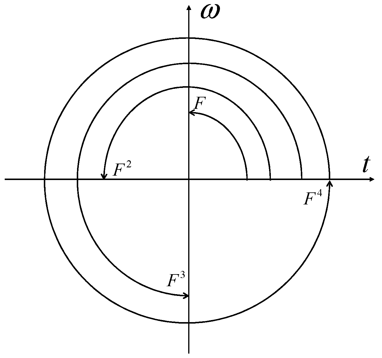
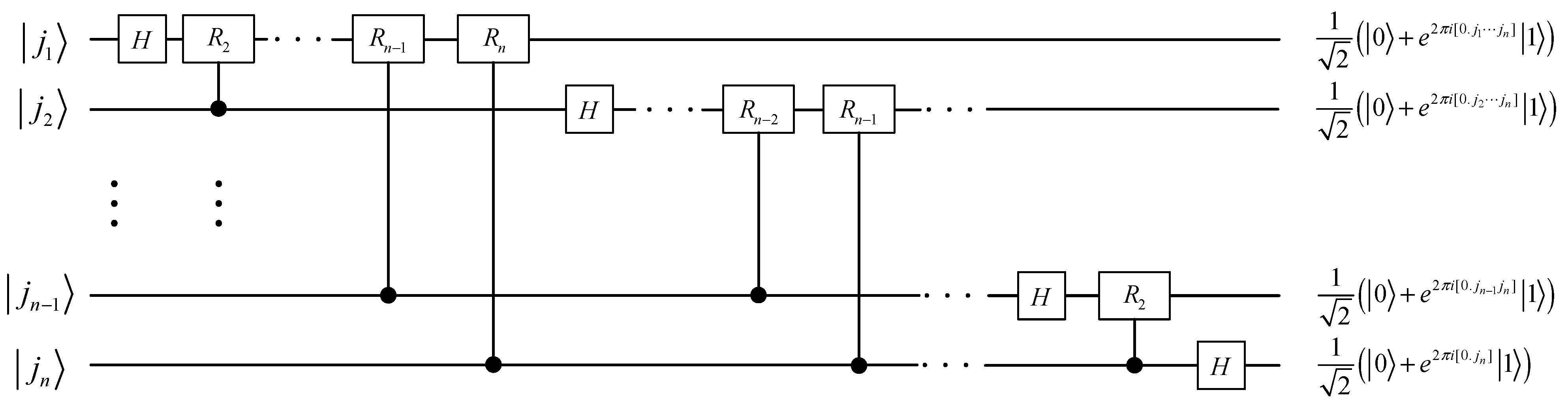
• The QFT is a unitary operator. The Fourier transform of a quantum state $|\alpha \rangle$ can be expressed as

  $$|\alpha \rangle ―QFT―|{\beta }_1\rangle$$
• The quadratic power of the QFT can be expressed as

  $${QFT}^2=\left(\begin{array}{cccc}1& 0& \dots & 0\\ 0& 0& \dots & 1\\ ⋮& ⋮& ⋰& ⋮\\ 0& 1& \dots & 0\end{array}\right)$$

For the vector $\left({\alpha }_0,{\alpha }_1,\dots ,{\alpha }_{n-1}\right)$, the transformation can be expressed as

$$\left({\alpha }_0,{\alpha }_1,\dots ,{\alpha }_{n-1}\right)\left(\begin{array}{cccc}1& 0& \dots & 0\\ 0& 0& \dots & 1\\ ⋮& ⋮& ⋰& ⋮\\ 0& 1& \dots & 0\end{array}\right)=\left({\alpha }_0,{\alpha }_{n-1},\dots ,{\alpha }_1\right)$$

In order to realize the quantum circuit of the above matrix, multiple swap gates are required. The swap gate of two quanta is shown in Figure 5.

Thus, for ${QFT}^2$, we provide quantum circuits of eight quantum states, as shown in Figure 6.

For a $2^n\times 2^n$ dimensional identity matrix, we can obtain the ${QFT}^2$ by row transformation, as shown in Figure 7.

Therefore, the quantum circuit of Figure 6 can be simplified as Figure 8.

Thus, the ${QFT}^2$ for quantum state $|\alpha \rangle$ can be expressed as

$$|\alpha \rangle ―{QFT}^2―|{\beta }_2\rangle$$

• The third power of the QFT, which is equivalent to the inverse operation of the QFT, is also a unitary operator.

  $$|\alpha \rangle ―{QFT}^3―|{\beta }_3\rangle$$

Therefore, the QWFRFT of the quantum state by Equation (10) can be expressed as

$$\begin{array}{ccc}\hfill QWFRFT\left(|\alpha \rangle \right)& =& \frac{1}{4}\left(I\left(|\alpha \rangle \right),QFT\left(|\alpha \rangle \right),{QFT}^2\left(|\alpha \rangle \right),{QFT}^3\left(|\alpha \rangle \right)\right)\left(\begin{array}{cccc}1& 1& 1& 1\\ 1& -i& -1& i\\ 1& -1& 1& -1\\ 1& i& -1& -i\end{array}\right)\left(\begin{array}{l}{B}_0^{\alpha }\\ B_1^{\alpha }\\ B_2^{\alpha }\\ B_3^{\alpha }\end{array}\right)\hfill \\ & =& \frac{1}{4}\left(|{\beta }_0\rangle ,|{\beta }_1\rangle ,|{\beta }_2\rangle ,|{\beta }_3\rangle \right)\left(\begin{array}{cccc}1& 1& 1& 1\\ 1& -i& -1& i\\ 1& -1& 1& -1\\ 1& i& -1& -i\end{array}\right)\left(\begin{array}{l}{B}_0^{\alpha }\\ B_1^{\alpha }\\ B_2^{\alpha }\\ B_3^{\alpha }\end{array}\right).\hfill \end{array}$$

(33)

Equation (33) can be further written as

$$\begin{array}{ccc}\hfill QWFRFT\left(|\alpha \rangle \right)& =& \frac{1}{4}\left(|{\beta }_0\rangle ,|{\beta }_1\rangle ,|{\beta }_2\rangle ,|{\beta }_3\rangle \right)\left(\begin{array}{cccc}1& 1& 1& 1\\ 1& -i& -1& i\\ 1& -1& 1& -1\\ 1& i& -1& -i\end{array}\right)\left(\begin{array}{l}{B}_0^{\alpha }\\ B_1^{\alpha }\\ B_2^{\alpha }\\ B_3^{\alpha }\end{array}\right)\hfill \\ & =& \frac{1}{4}\left(|{\beta }_0\rangle ,|{\beta }_1\rangle ,|{\beta }_2\rangle ,|{\beta }_3\rangle \right)\left(\begin{array}{cccc}\exp \left(\frac{-2\pi i0\times 0}{4}\right)& \exp \left(\frac{-2\pi i0\times 1}{4}\right)& \exp \left(\frac{-2\pi i0\times 2}{4}\right)& \exp \left(\frac{-2\pi i0\times 3}{4}\right)\\ \exp \left(\frac{-2\pi i1\times 0}{4}\right)& \exp \left(\frac{-2\pi i1\times 1}{4}\right)& \exp \left(\frac{-2\pi i1\times 2}{4}\right)& \exp \left(\frac{-2\pi i1\times 3}{4}\right)\\ \exp \left(\frac{-2\pi i2\times 0}{4}\right)& \exp \left(\frac{-2\pi i2\times 1}{4}\right)& \exp \left(\frac{-2\pi i2\times 2}{4}\right)& \exp \left(\frac{-2\pi i2\times 3}{4}\right)\\ \exp \left(\frac{-2\pi i3\times 0}{4}\right)& \exp \left(\frac{-2\pi i3\times 1}{4}\right)& \exp \left(\frac{-2\pi i3\times 2}{4}\right)& \exp \left(\frac{-2\pi i3\times 3}{4}\right)\end{array}\right)\left(\begin{array}{l}{B}_0^{\alpha }\\ B_1^{\alpha }\\ B_2^{\alpha }\\ B_3^{\alpha }\end{array}\right)\hfill \end{array}$$

(34)

where $B_k^{\alpha }=\exp \left(\frac{2\pi ik\alpha }{4}\right)$; $k=0,1,2,3$. Then, Equation (34) can be written again as

$$\begin{array}{ccc}\hfill QWFRFT\left(|\alpha \rangle \right)& =& \frac{1}{4}{\displaystyle \sum _{l=0}^3{\displaystyle \sum _{k=0}^3|{\beta }_l\rangle \exp \left(\frac{-2\pi ilk}{4}\right)}}{B}_k^{\alpha }\hfill \\ & =& \frac{1}{4}{\displaystyle \sum _{l=0}^3{\displaystyle \sum _{k=0}^3|{\beta }_l\rangle \exp \left(\frac{-2\pi ilk}{4}\right)}}\exp \left(\frac{2\pi ik\alpha }{4}\right)\hfill \\ & =& \frac{1}{4}{\displaystyle \sum _{l=0}^3{\displaystyle \sum _{k=0}^3|{\beta }_l\rangle \exp \left(\frac{2\pi ik\left(\alpha -l\right)}{4}\right)}}.\hfill \end{array}$$

(35)

With the help of the quantum artificial neural network (QANN), we are inspired to design a QWFRFT. Here, we first introduce the QANN [34,35]. If we use $\left\{|e_1\rangle ,|e_2\rangle ,\dots ,|e_M\rangle \right\}$ to denote the canonical basis for ${ℂ}^M$, then the quantum artificial neural network above can be rewritten as

$$Q\left(|x\rangle \right)={\displaystyle \sum _{k=1}^M{\displaystyle \sum _{j=1}^N\left({\alpha }_{j,k}^{\left(1\right)}{\sigma }_k\left(\langle w_{j,k}^{\left(1\right)}|T|x\rangle +{\theta }_{j,k}^{\left(1\right)}\right)+i{\alpha }_{j,k}^{\left(2\right)}{\sigma }_k\left(\langle w_{j,k}^{\left(2\right)}|T|x\rangle +{\theta }_{j,k}^{\left(2\right)}\right)\right)}}|e_k\rangle .$$

(36)

Put $y_{j,k}^{\left(i\right)}={\sigma }_k\left({\displaystyle \sum _{t=1}^n\langle w_{j,k}^{\left(i\right)}\left(t\right)|T|x_t\rangle +{\theta }_{j,k}^{\left(i\right)}}\right)$ and $|{\alpha }_k^{\left(i\right)}\rangle ={\displaystyle \sum _{j=1}^N{\alpha }_{j,k}^{\left(i\right)}{y}_{j,k}^{\left(i\right)}|e_k\rangle }$. Then, a QANN can be illustrated by Figure 9 and Figure 10 below.

Thus, we can present the circuit of the QWFRFT, as shown in Figure 11.

So far, we have completed the QWFRFT and circuit implementation. The work of this paper is a supplement to the work of Parasa et al. At one point, researchers pointed out that there is no quantum-weighted fractional Fourier transform [32]. However, our study illustrates the diversity of FRFT and proposes QWFRFT. Due to the characteristics of quantum parallelism, we believe that the QWFRFT has a wider application space.

At present, our method is only applicable to closed systems. The standard quantum theory has shown its limit to describe successfully experimental results. Counterintuitive results are obtained in different experiments [36,37]. The open system effects need to be further analyzed.

5. Conclusions

Unitarity is a prerequisite for the realization of quantum algorithms. In this paper, we proposed the reformulation of the WFRFT. The unitarity of the WFRFT was proved by means of the proposed reformulation. The QFT is an important part of the QWFRFT. Furthermore, we presented the integer power operation and quantum circuit of the QFT, which lays the foundation for the QWFRFT. Finally, we designed the circuit of the QWFRFT with the help of a quantum artificial neural network and proposed the electronic circuit of the QWFRFT. The results of this paper show that there is a QFRFT algorithm, which lays the foundation for further research.

References

1. Feynman, R.P. Simulating physics with computers. Int. J. Theor. Phys 1982, 21, 467–488. [Google Scholar] [CrossRef]
2. Deutsch, D. Quantum theory, the Church–Turing principle and the universal quantum computer. Proc. R. Soc. Lond. A Math. Phys. Sci. 1985, 400, 97–117. [Google Scholar]
3. Shor, P.W. Algorithms for quantum computation: Discrete logarithms and factoring. In Proceedings of the 35th Annual IEEE Symposium on Foundations of Computer Science, Santa Fe, NM, USA, 20–22 November 1994; pp. 124–134. [Google Scholar]
4. Shor, P.W. Polynomial-time algorithms for prime factorization and discrete logarithms on a quantum computer. SIAM Rev. 1999, 41, 303–332. [Google Scholar] [CrossRef]
5. Grover, L.K. A fast quantum mechanical algorithm for database search. In Proceedings of the 28th Annual ACM Symposium on the Theory of Computing, New York, NY, USA, 22–24 May 1996; pp. 212–219. [Google Scholar]
6. Biham, E.; Biham, O.; Biron, D.; Grassl, M.; Lidar, D.A. Grover’s quantum search algorithm for an arbitrary initial amplitude distribution. Phys. Rev. A 1999, 60, 2742–2745. [Google Scholar] [CrossRef] [Green Version]
7. Boyer, M.; Brassard, G.; Høyer, P.; Tapp, A. Tight bounds on quantum searching. Fortschr. Der Phys. Prog. Phys. 1998, 46, 493–505. [Google Scholar] [CrossRef] [Green Version]
8. Grover, L.K. Quantum computers can search rapidly by using almost any transformation. Phys. Rev. Lett. 1998, 80, 4329–4332. [Google Scholar] [CrossRef] [Green Version]
9. GuiLu, L.; WeiLin, Z.; YanSong, L.; Li, N. Arbitrary phase rotation of the marked state cannot be used for Grover’s quantum search algorithm. Commun. Theor. Phys. 1999, 32, 335–338. [Google Scholar] [CrossRef] [Green Version]
10. Long, G.L.; Li, Y.S.; Zhang, W.L.; Niu, L. Phase matching in quantum searching. Phys. Lett. A 1999, 262, 27–34. [Google Scholar] [CrossRef] [Green Version]
11. Narayanan, A.; Moore, M. Quantum-inspired genetic algorithms. In Proceedings of the IEEE International Conference on Evolutionary Computation, Nagoya, Japan, 20–22 May 1996; pp. 61–66. [Google Scholar]
12. Shenvi, N.; Kempe, J.; Whaley, K.B. Quantum random-walk search algorithm. Phys. Rev. A 2003, 67, 052307. [Google Scholar] [CrossRef] [Green Version]
13. Han, K.-H.; Kim, J.-H. Genetic quantum algorithm and its application to combinatorial optimization problem. In Proceedings of the IEEE Congress on Evolutionary Computation, La Jolla, CA, USA, 16–19 July 2000; pp. 1354–1360. [Google Scholar]
14. Chen, L.B. Mitochondrial membrane potential in living cells. Annu. Rev. Cell Biol. 1988, 4, 155–181. [Google Scholar] [CrossRef]
15. Høyer, P.; Špalek, R. Quantum fan-out is powerful. Theory Comput. 2005, 1, 81–103. [Google Scholar] [CrossRef]
16. Sun, J.; Wu, X.; Palade, V.; Fang, W.; Lai, C.-H.; Xu, W. Convergence analysis and improvements of quantum-behaved particle swarm optimization. Inf. Sci. 2012, 193, 81–103. [Google Scholar] [CrossRef]
17. Harrow, A.W.; Hassidim, A.; Lloyd, S. Quantum algorithm for linear systems of equations. Phys. Rev. Lett. 2009, 103, 150502. [Google Scholar] [CrossRef] [PubMed]
18. Childs, A.M.; Kothari, R.; Somma, R.D. Quantum algorithm for systems of linear equations with exponentially improved dependence on precision. SIAM J. Comput. 2017, 46, 1920–1950. [Google Scholar] [CrossRef] [Green Version]
19. Clader, B.D.; Jacobs, B.C.; Sprouse, C.R. Preconditioned quantum linear system algorithm. Phys. Rev. Lett. 2013, 110, 250504. [Google Scholar] [CrossRef] [Green Version]
20. Wossnig, L.; Zhao, Z.; Prakash, A. Quantum linear system algorithm for dense matrices. Phys. Rev. Lett. 2018, 120, 050502. [Google Scholar] [CrossRef] [Green Version]
21. Arrazola, J.M.; Kalajdzievski, T.; Weedbrook, C.; Lloyd, S. Quantum algorithm for nonhomogeneous linear partial differential equations. Phys. Rev. A 2019, 100, 032306. [Google Scholar] [CrossRef] [Green Version]
22. Lloyd, S.; De Palma, G.; Gokler, C.; Kiani, B.; Liu, Z.-W.; Marvian, M.; Tennie, F.; Palmer, T. Quantum algorithm for nonlinear differential equations. arXiv 2020, arXiv:2011.06571. [Google Scholar]
23. Childs, A.M.; Liu, J.-P. Quantum spectral methods for differential equations. Commun. Math. Phys. 2020, 375, 1427–1457. [Google Scholar] [CrossRef] [Green Version]
24. Childs, A.M.; Liu, J.-P.; Ostrander, A. High-precision quantum algorithms for partial differential equations. Quantum 2021, 5, 574. [Google Scholar] [CrossRef]
25. Coppersmith, D. An approximate Fourier transform useful in quantum factoring. arXiv 2002, arXiv:quant-ph/0201067. [Google Scholar]
26. Nielsen, M.A.; Chuang, I.L. Quantum computation and quantum information. Phys. Today 2001, 54, 60. [Google Scholar]
27. Biamonte, J.; Wittek, P.; Pancotti, N.; Rebentrost, P.; Wiebe, N.; Lloyd, S. Quantum machine learning. Nature 2017, 549, 195–202. [Google Scholar] [CrossRef] [PubMed]
28. Namias, V. The fractional order Fourier transform and its application to quantum mechanics. IMA J. Appl. Math. 1980, 25, 241–265. [Google Scholar] [CrossRef]
29. Candan, C.; Kutay, M.A.; Ozaktas, H.M. The discrete fractional Fourier transform. IEEE Trans. Signal Process. 2000, 48, 1329–1337. [Google Scholar] [CrossRef] [Green Version]
30. Shih, C.C. Fractionalization of Fourier transform. Opt. Commun. 1995, 118, 495–498. [Google Scholar] [CrossRef]
31. Ozaktas, H.M.; Arikan, O.; Kutay, M.A.; Bozdagt, G. Digital computation of the fractional Fourier transform. IEEE Trans. Signal Process. 1996, 44, 2141–2150. [Google Scholar] [CrossRef] [Green Version]
32. Parasa, V.; Perkowski, M. Quantum pseudo-fractional fourier transform using multiple-valued logic. In Proceedings of the IEEE 42nd International Symposium on Multiple-Valued Logic, Victoria, BC, Canada, 14–16 May 2012; pp. 311–314. [Google Scholar]
33. Bailey, D.H.; Swarztrauber, P.N. The fractional Fourier transform and applications. SIAM Rev. 1991, 33, 389–404. [Google Scholar] [CrossRef]
34. Cao, H.; Cao, F.; Wang, D. Quantum artificial neural networks with applications. Inf. Sci. 2015, 290, 1–6. [Google Scholar] [CrossRef]
35. da Silva, A.J.; de Oliveira, W.R. Comments on “quantum artificial neural networks with applications”. Inf. Sci. 2016, 370, 120–122. [Google Scholar] [CrossRef]
36. Eleuch, H.; Rotter, I. Nearby states in non-Hermitian quantum systems I: Two states. Eur. Phys. J. D 2015, 69, 229. [Google Scholar] [CrossRef] [Green Version]
37. Eleuch, H.; Rotter, I. Clustering of exceptional points and dynamical phase transitions. Phys. Rev. A 2016, 93, 042116. [Google Scholar] [CrossRef] [Green Version]
Figure 1. A circuit for phase estimation.
Mathematics 10 01896 g001
Figure 2. Time–frequency representation of Fourier transform.
Mathematics 10 01896 g002
Figure 3. The reformulation of the WFRFT module.
Mathematics 10 01896 g003
Figure 4. A circuit for the QFT.
Mathematics 10 01896 g004
Figure 5. Swap gate.
Mathematics 10 01896 g005
Figure 6. A circuit forthe Q F T 2 .
Mathematics 10 01896 g006
Figure 7. Matrix of the Q F T 2 .
Mathematics 10 01896 g007
Figure 8. A circuit for the Q F T 2 .
Mathematics 10 01896 g008
Figure 9. The output | α k ( i ) of a QANN, where i = 1 , 2 ; k = 1 , 2 , , M .
Mathematics 10 01896 g009
Figure 10. The output Q ( | x ) of a QANN.
Mathematics 10 01896 g010
Figure 11. A circuit for the QWFRFT.
Mathematics 10 01896 g011
Publisher’s Note: MDPI stays neutral with regard to jurisdictional claims in published maps and institutional affiliations.