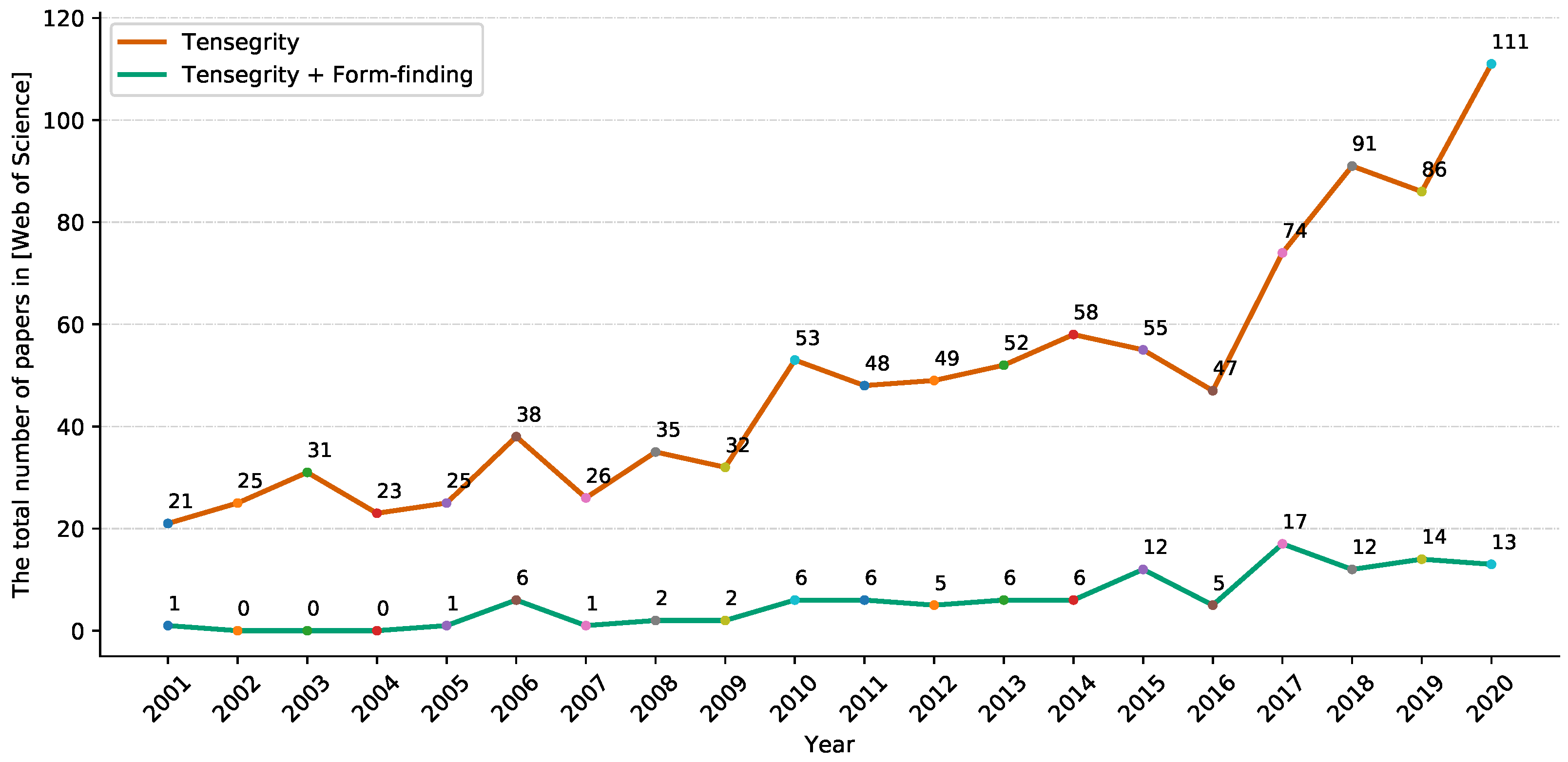
Figure 1.
The total number of articles and papers on the Web of Science homepage. Results using subjects, ‘Tensegrity’ and ‘Tensegrity + Form-finding’.
Figure 1.
The total number of articles and papers on the Web of Science homepage. Results using subjects, ‘Tensegrity’ and ‘Tensegrity + Form-finding’.
Figure 2.
A 2D two-strut tensegrity structure in which cables and struts are denoted by the thin and thick lines.
Figure 2.
A 2D two-strut tensegrity structure in which cables and struts are denoted by the thin and thick lines.
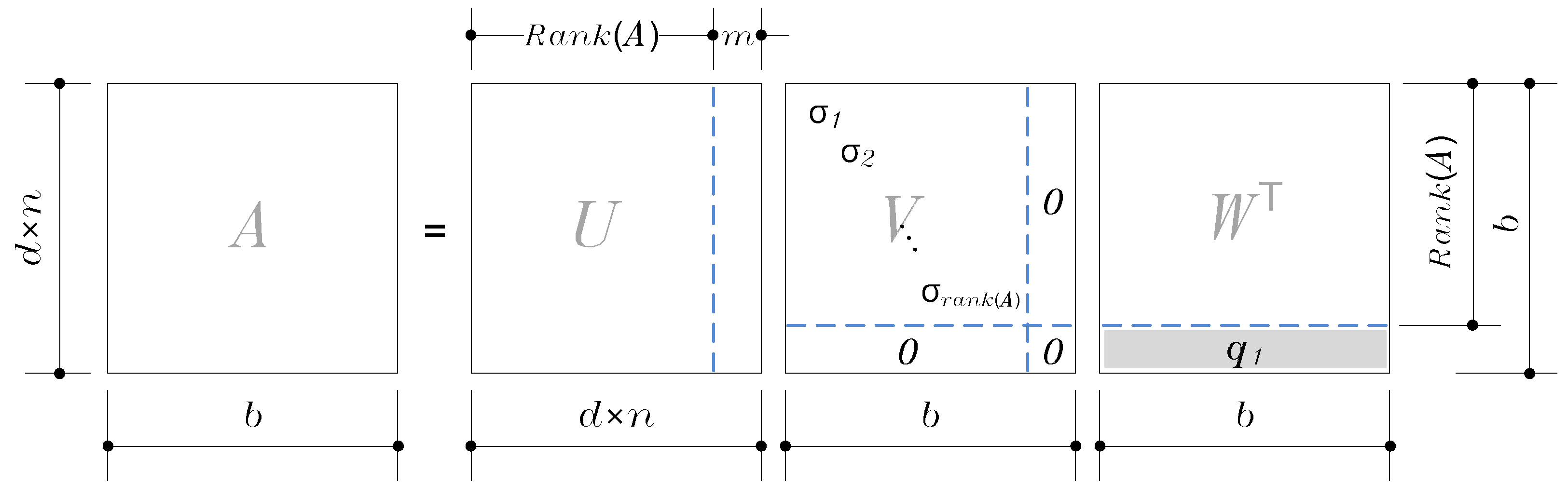
Figure 3.
Graphical illustration of the SVD of the equilibrium matrix A.
Figure 3.
Graphical illustration of the SVD of the equilibrium matrix A.
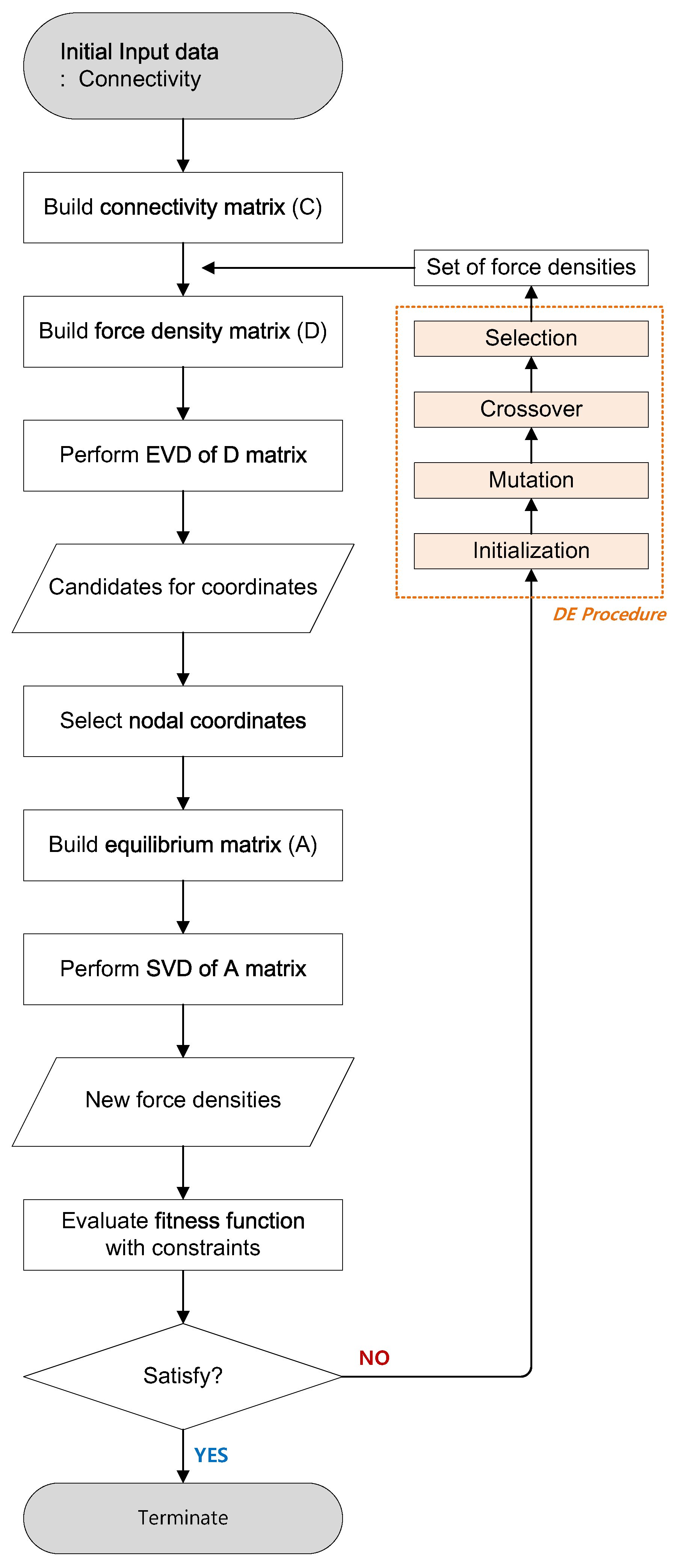
Figure 4.
Flowchart of the conventional form-finding process of tensegrity structures using the FDM.
Figure 4.
Flowchart of the conventional form-finding process of tensegrity structures using the FDM.
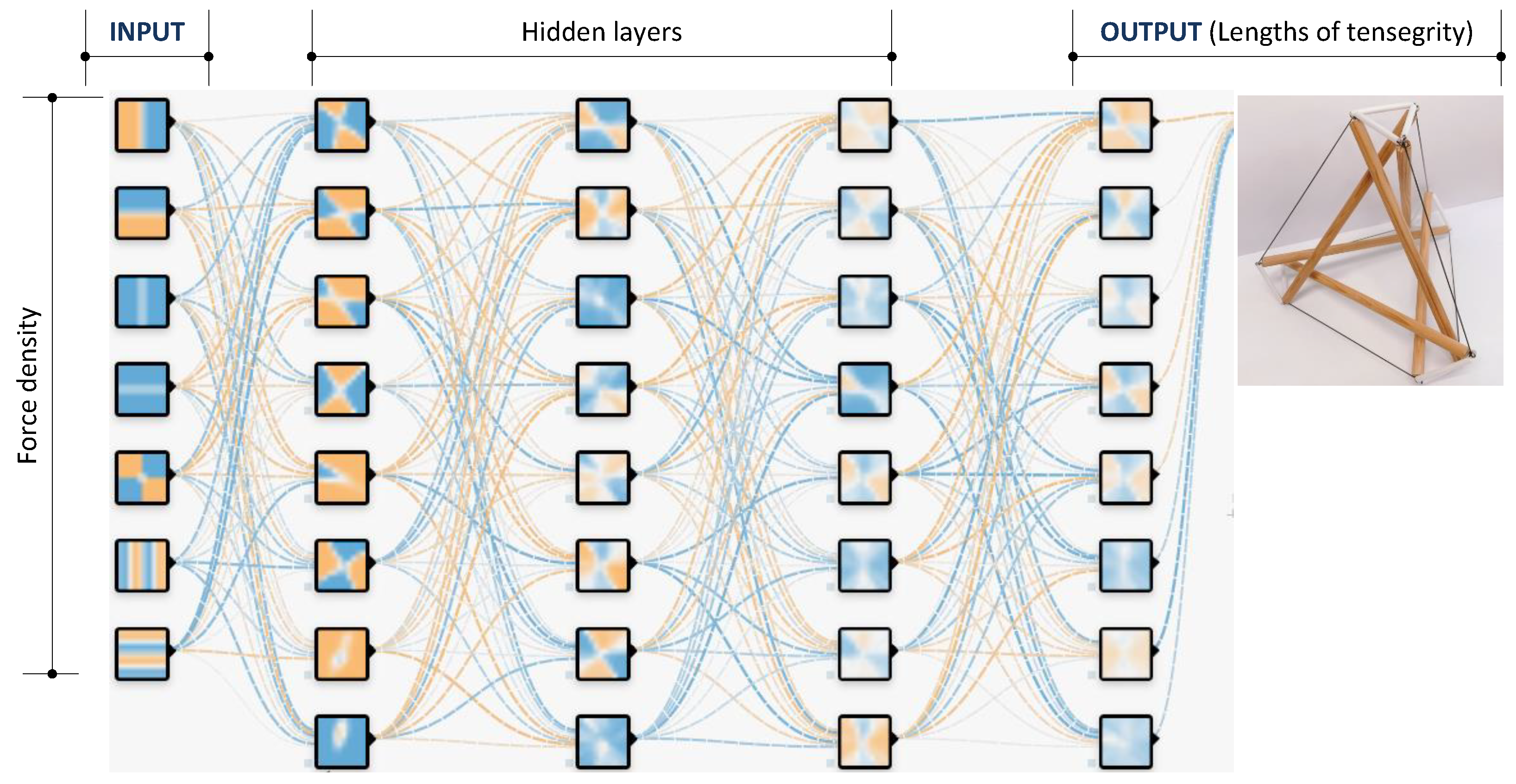
Figure 5.
The DNN models with input and output layers denoted for the force densities and lengths of the elements, respectively.
Figure 5.
The DNN models with input and output layers denoted for the force densities and lengths of the elements, respectively.
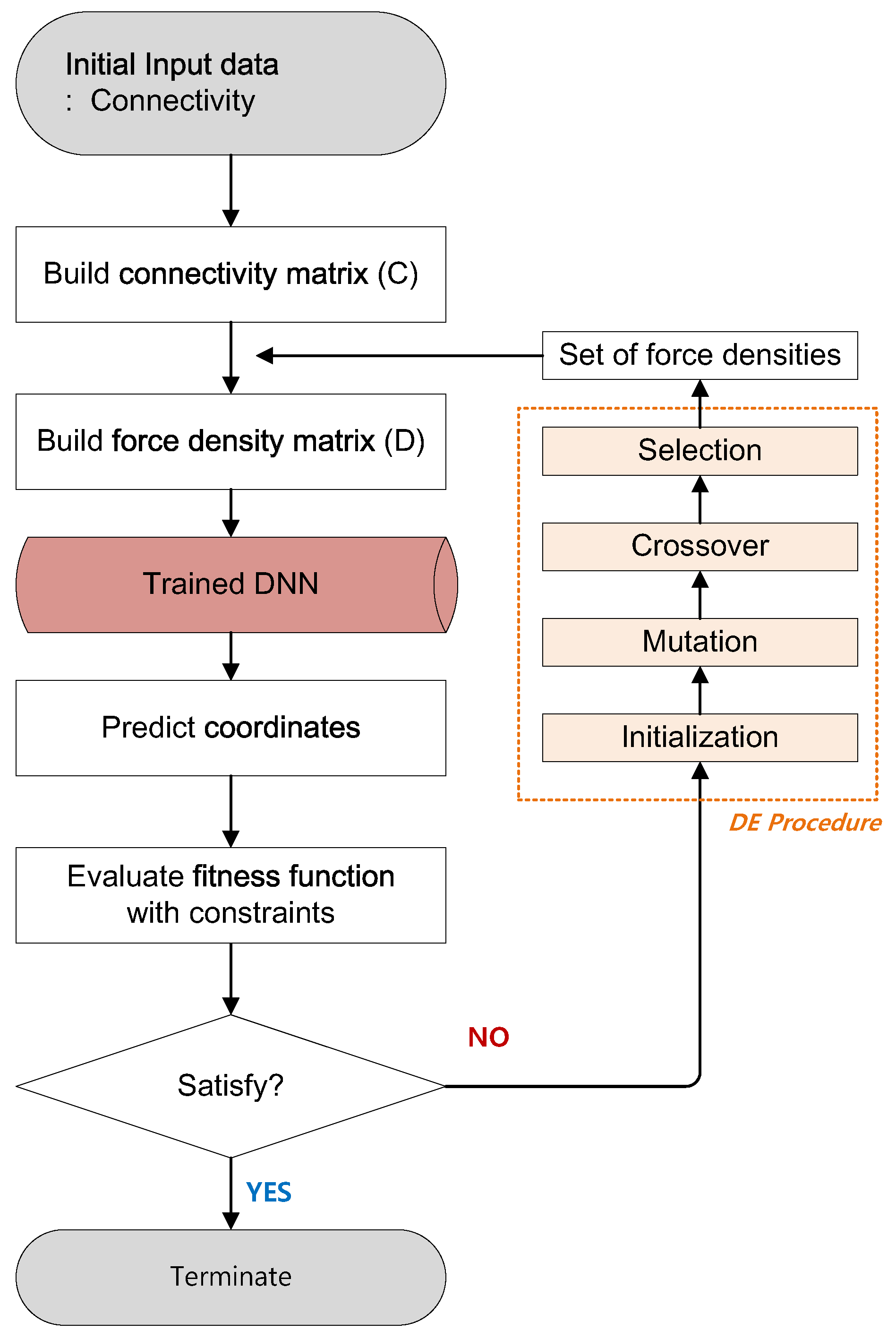
Figure 6.
Flowchart of the DNN-based form-finding process of tensegrity structures to eliminate the calculation of EVD and SVD.
Figure 6.
Flowchart of the DNN-based form-finding process of tensegrity structures to eliminate the calculation of EVD and SVD.
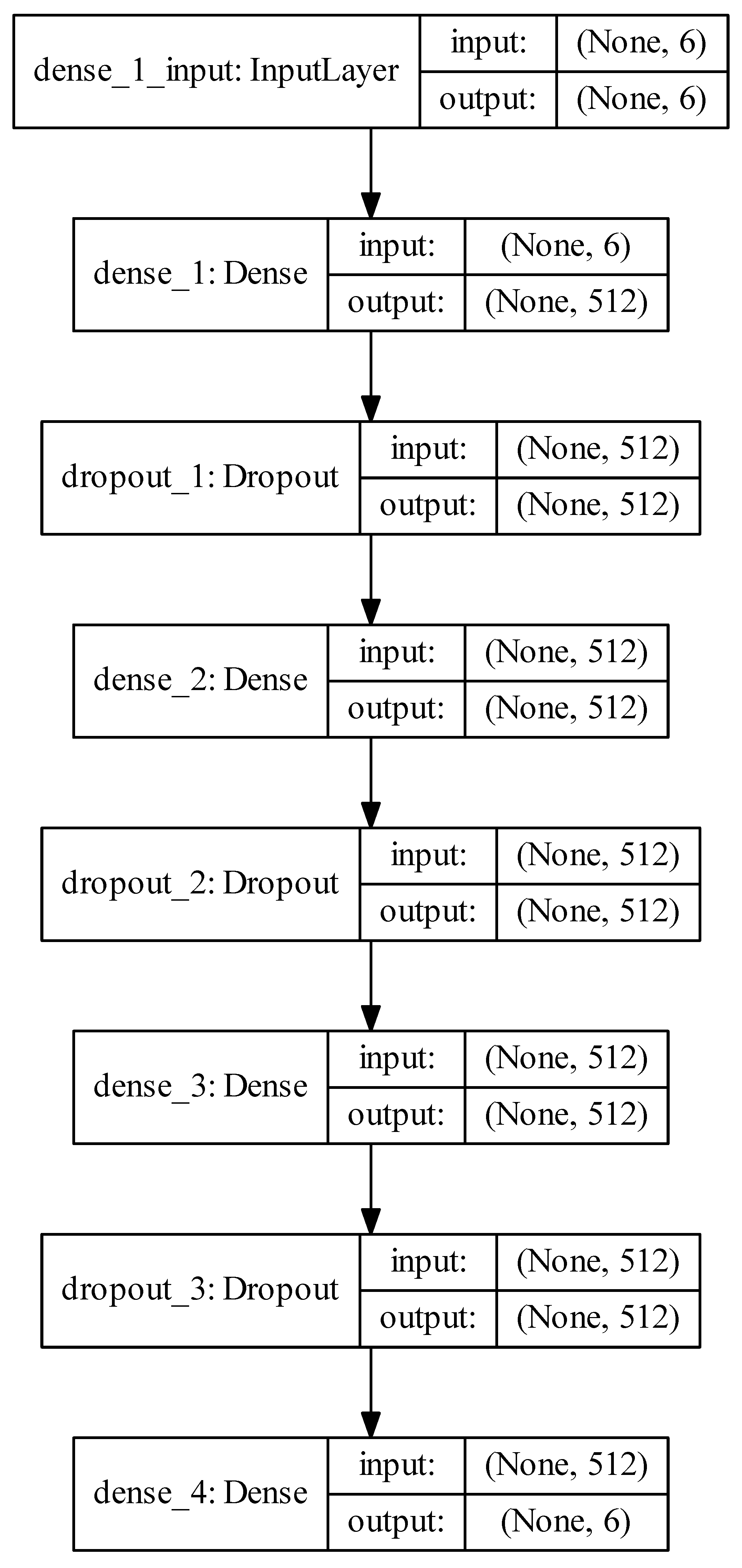
Figure 7.
Visualization of the DNN for training the 2D two-strut tensegrity structure.
Figure 7.
Visualization of the DNN for training the 2D two-strut tensegrity structure.
Figure 8.
The final results of 2D two-strut tensegrity structure using the (a) FDM and (b) DNN-based form-finding model with DE algorithm.
Figure 8.
The final results of 2D two-strut tensegrity structure using the (a) FDM and (b) DNN-based form-finding model with DE algorithm.
Figure 9.
Designation process of the nodal coordinates of the 2D two-strut tensegrity structure.
Figure 9.
Designation process of the nodal coordinates of the 2D two-strut tensegrity structure.
Figure 10.
Connectivity of the 3D-truncated tetrahedron tensegrity.
Figure 10.
Connectivity of the 3D-truncated tetrahedron tensegrity.
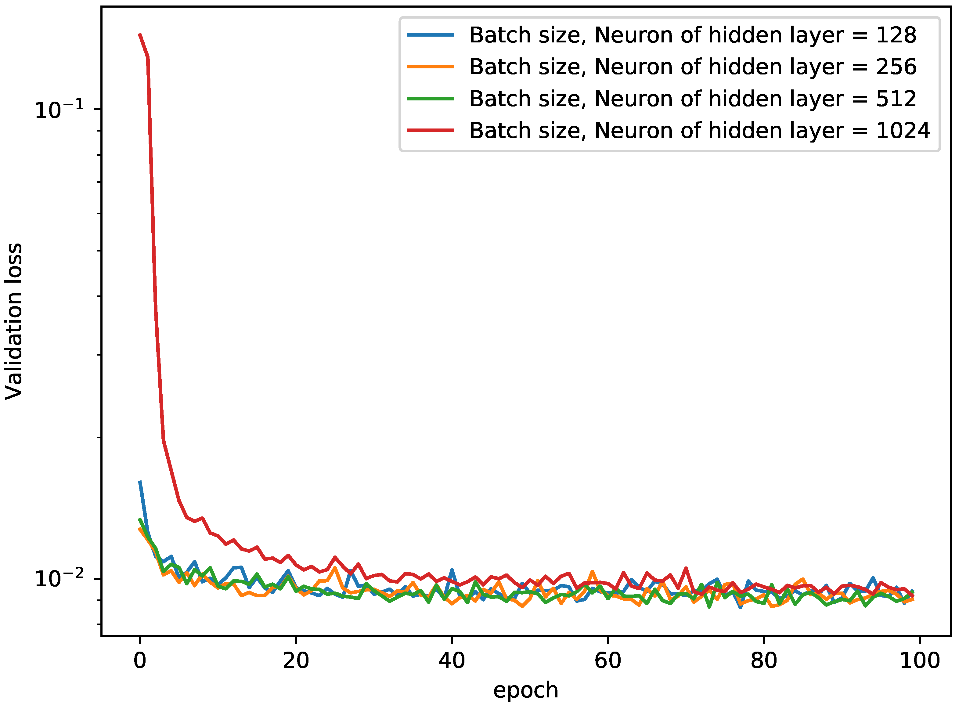
Figure 11.
Comparison of the validation loss for various mini-batch sizes with log-scale for 3D-truncated tetrahedron tensegrity.
Figure 11.
Comparison of the validation loss for various mini-batch sizes with log-scale for 3D-truncated tetrahedron tensegrity.
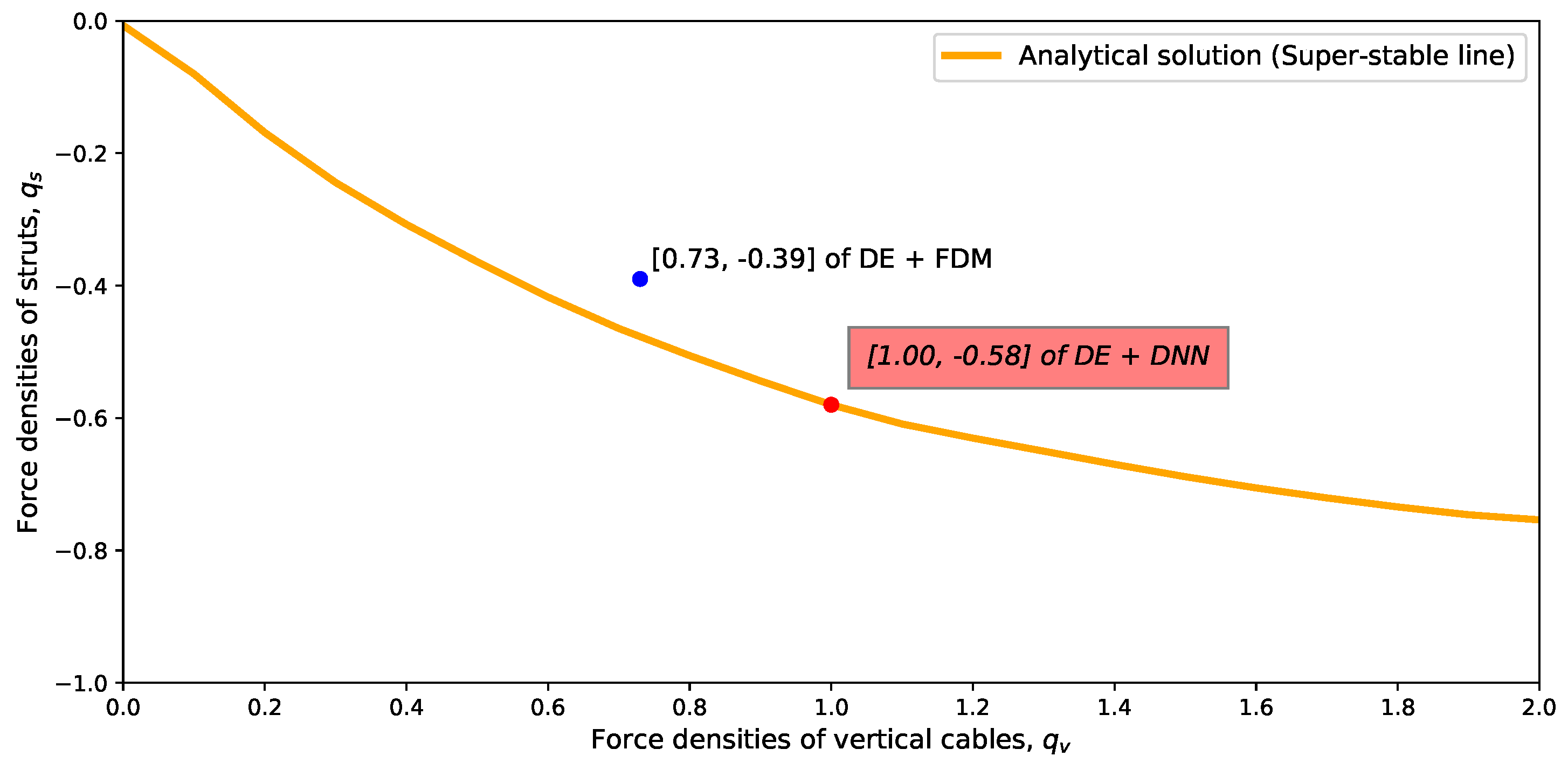
Figure 12.
Comparison of the force densities of the 3D truncated tetrahedron tensegrity using an FDM, a DNN-based form-finding model with a DE algorithm and a analytical solution [
6].
Figure 12.
Comparison of the force densities of the 3D truncated tetrahedron tensegrity using an FDM, a DNN-based form-finding model with a DE algorithm and a analytical solution [
6].
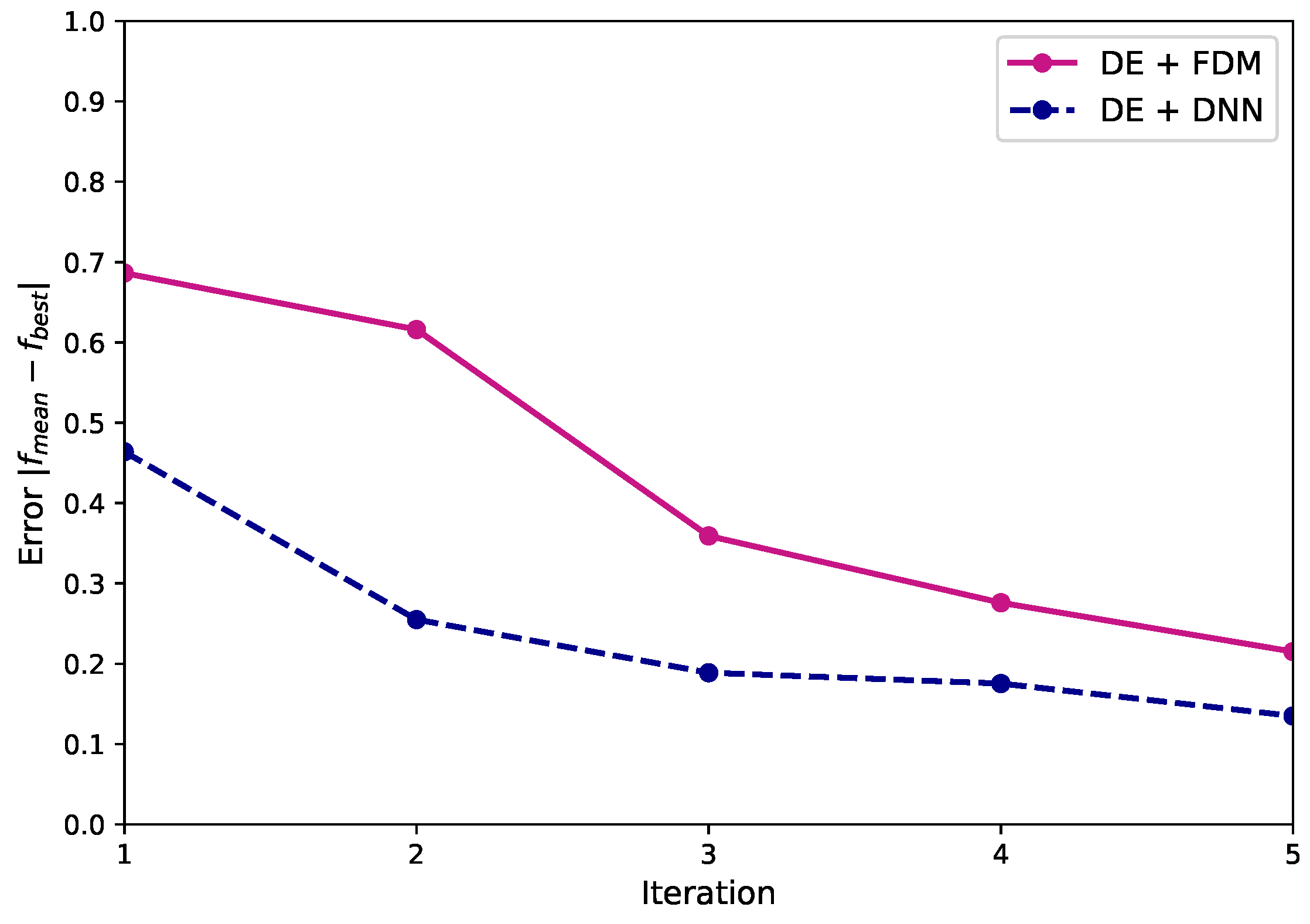
Figure 13.
Relationship between the iteration and error for the 3D-truncated tetrahedron tensegrity using an FDM and a DNN-based form-finding method with a DE algorithm.
Figure 13.
Relationship between the iteration and error for the 3D-truncated tetrahedron tensegrity using an FDM and a DNN-based form-finding method with a DE algorithm.
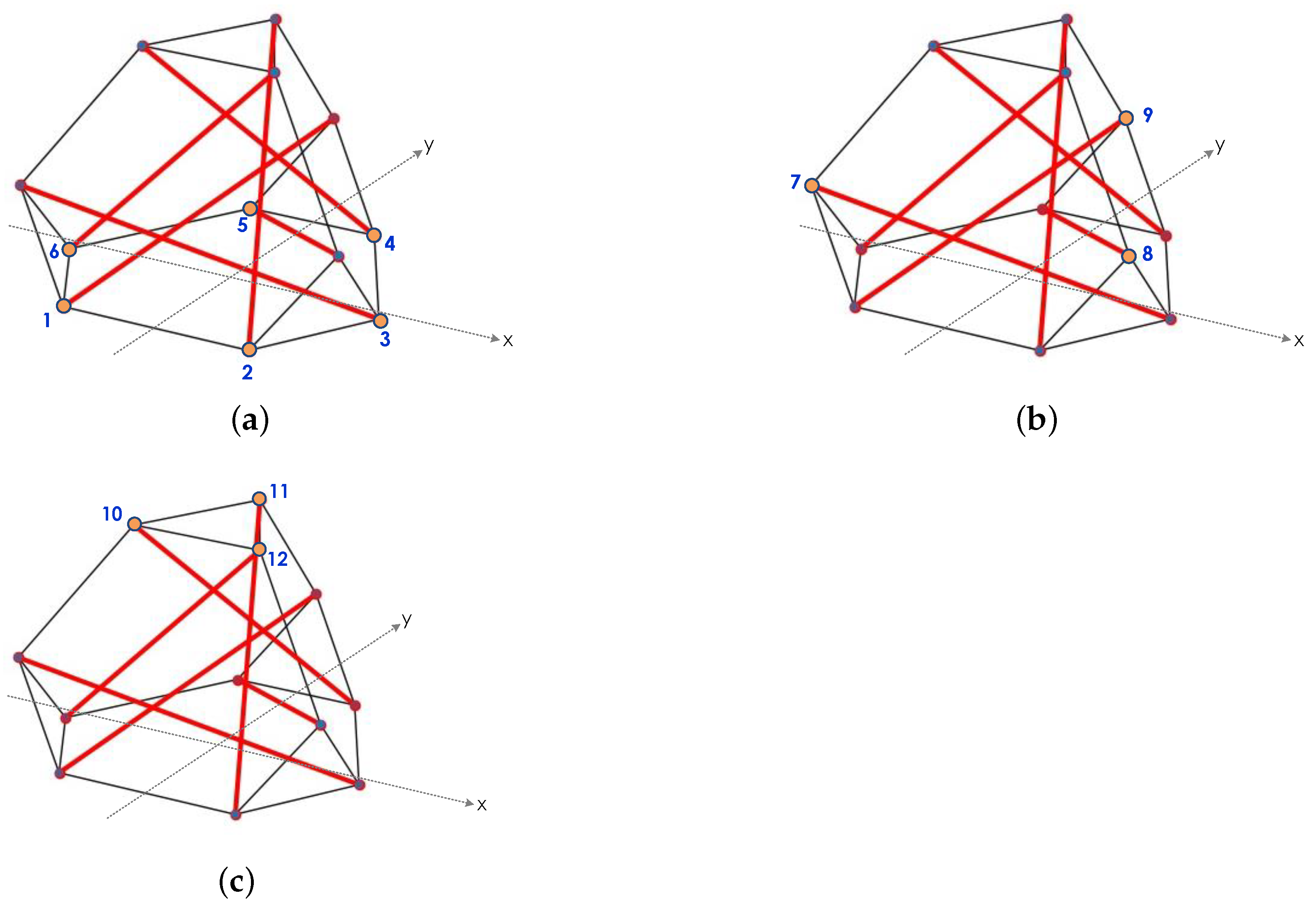
Figure 14.
Three steps of the coordinate designation for the 3D-truncated tetrahedron tensegrity. (a) Step 1: Nodes 1 to 6. (b) Step 2: Nodes 7 to 9. (c) Step 3: Nodes 10 to 12.
Figure 14.
Three steps of the coordinate designation for the 3D-truncated tetrahedron tensegrity. (a) Step 1: Nodes 1 to 6. (b) Step 2: Nodes 7 to 9. (c) Step 3: Nodes 10 to 12.
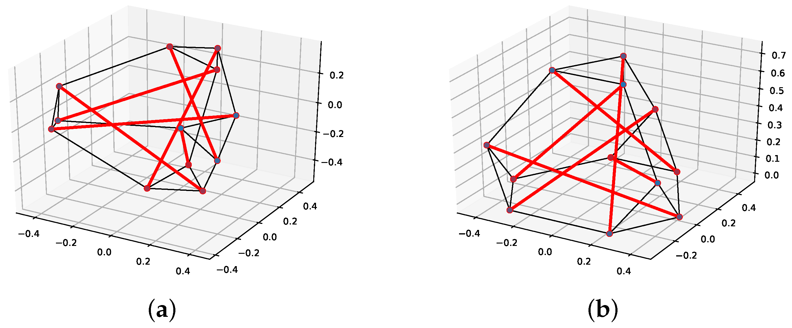
Figure 15.
Final geometry of five iterations of the 3D truncated tetrahedron tensegrity using an FDM and a DNN-based form-finding model with a DE algorithm. (a) FDM. (b) DNN-based form-finding model.
Figure 15.
Final geometry of five iterations of the 3D truncated tetrahedron tensegrity using an FDM and a DNN-based form-finding model with a DE algorithm. (a) FDM. (b) DNN-based form-finding model.
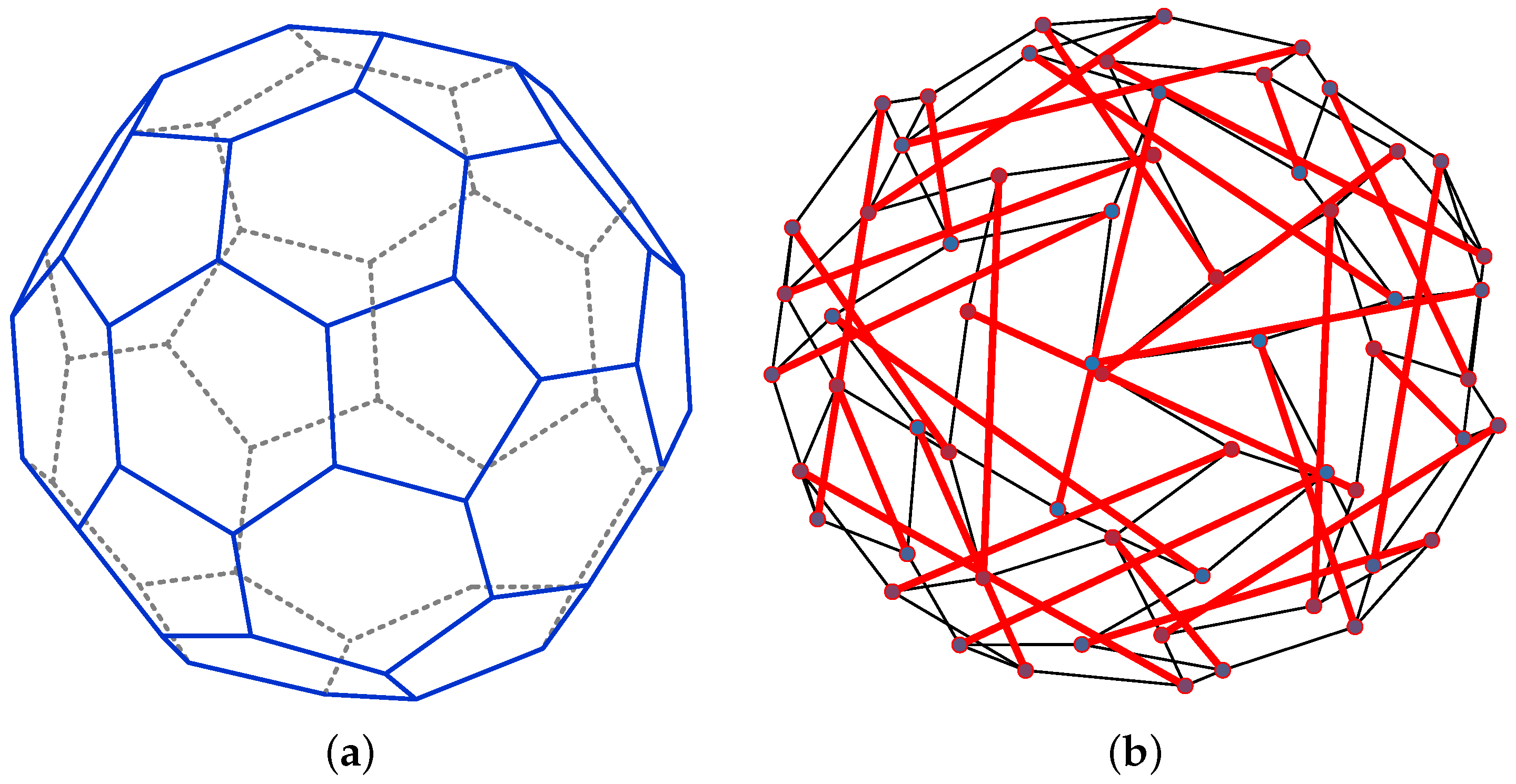
Figure 16.
3D-truncated icosahedron tensegrity in which the red thick lines denote strut members, and others are cable members. (a) Geometry. (b) Isometric view.
Figure 16.
3D-truncated icosahedron tensegrity in which the red thick lines denote strut members, and others are cable members. (a) Geometry. (b) Isometric view.
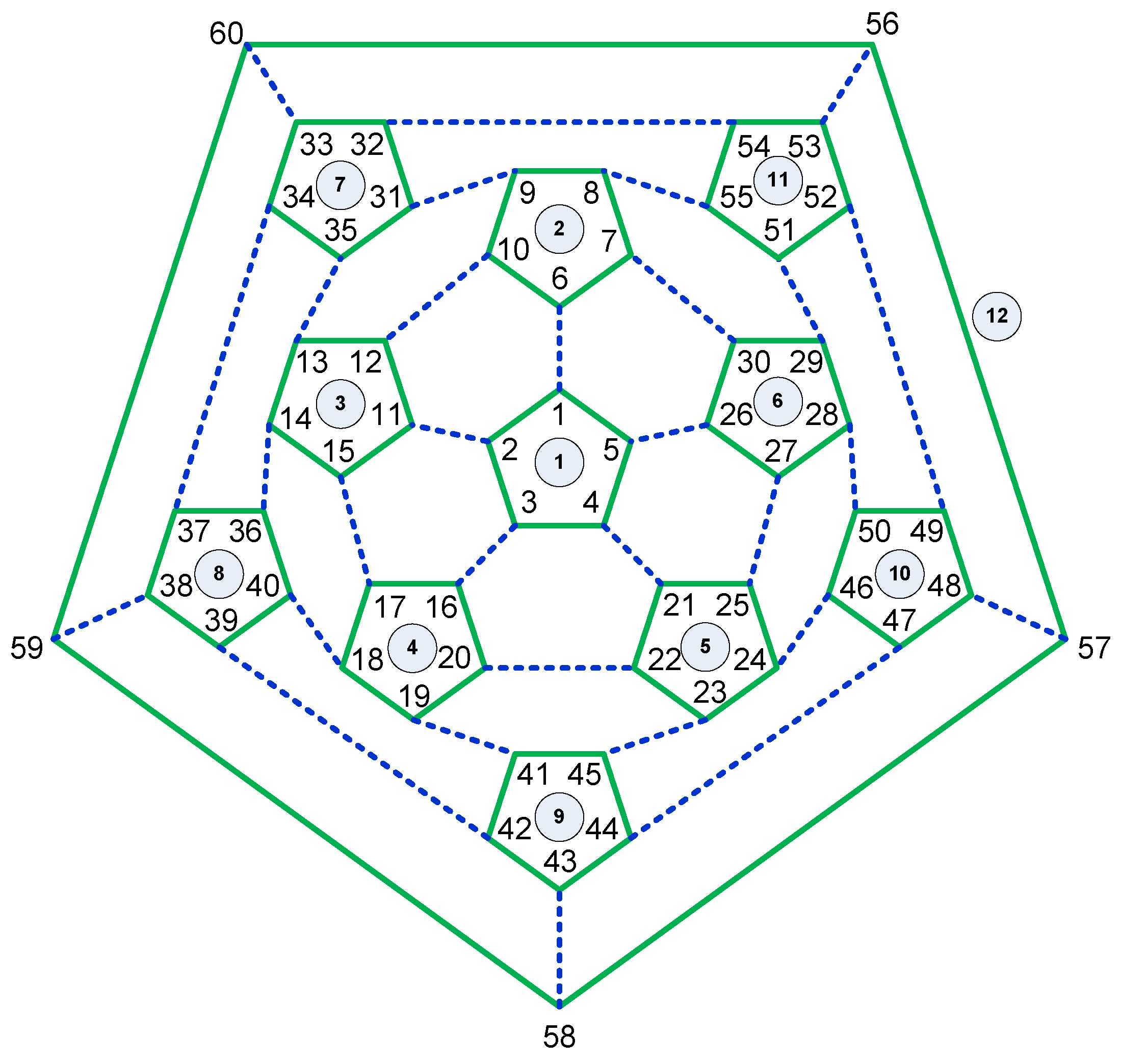
Figure 17.
Connectivity of the 3D-truncated tetrahedron tensegrity in which the blue dotted lines denote vertical cables, and others represent edge cables.
Figure 17.
Connectivity of the 3D-truncated tetrahedron tensegrity in which the blue dotted lines denote vertical cables, and others represent edge cables.
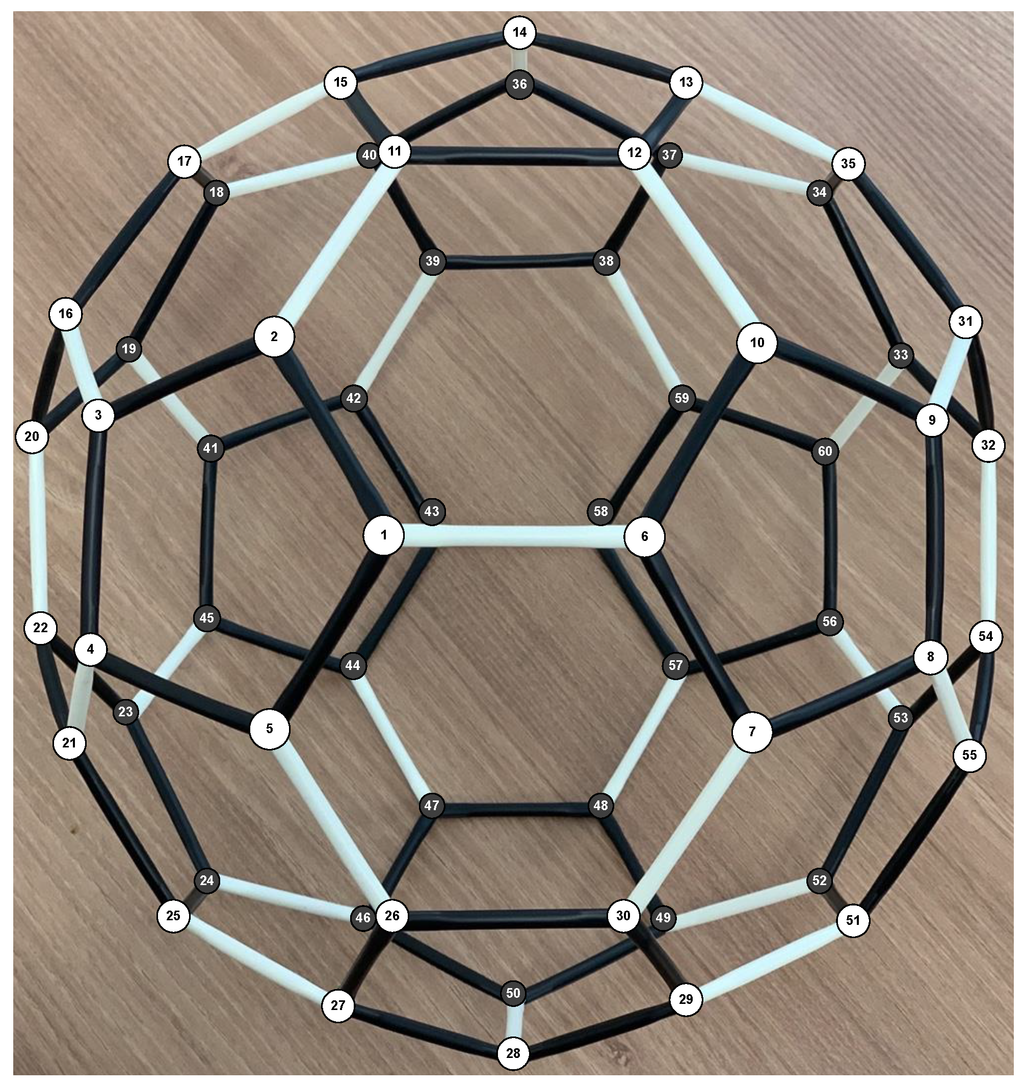
Figure 18.
The nodal points of the 3D-truncated tetrahedron tensegrity are numbered on the model.
Figure 18.
The nodal points of the 3D-truncated tetrahedron tensegrity are numbered on the model.
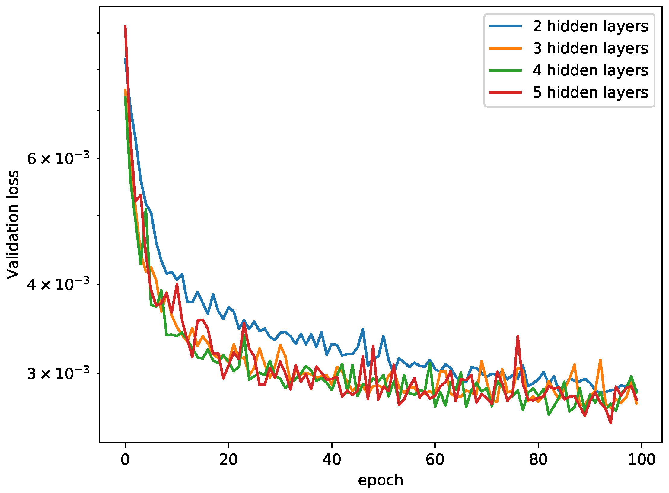
Figure 19.
Comparison of the validation loss for various hidden layer sizes with log-scale. The number of neurons is 512 for the 3D-truncated icosahedron tensegrity.
Figure 19.
Comparison of the validation loss for various hidden layer sizes with log-scale. The number of neurons is 512 for the 3D-truncated icosahedron tensegrity.
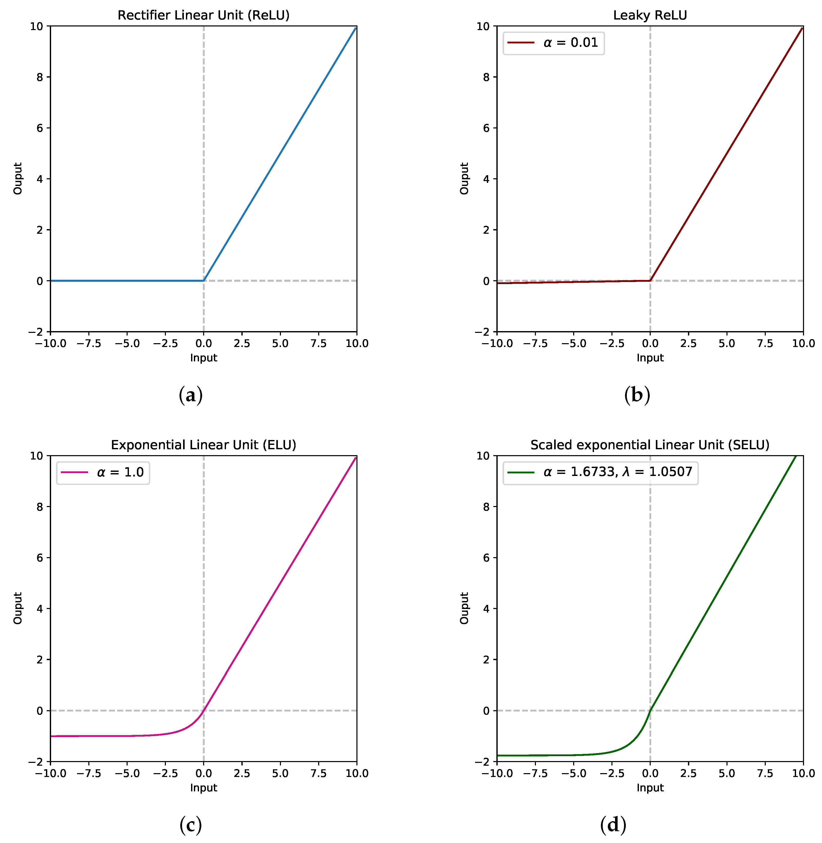
Figure 20.
Variants of activation functions. (a) ReLU. (b) Leaky ReLU. (c) ELU. (d) SELU.
Figure 20.
Variants of activation functions. (a) ReLU. (b) Leaky ReLU. (c) ELU. (d) SELU.
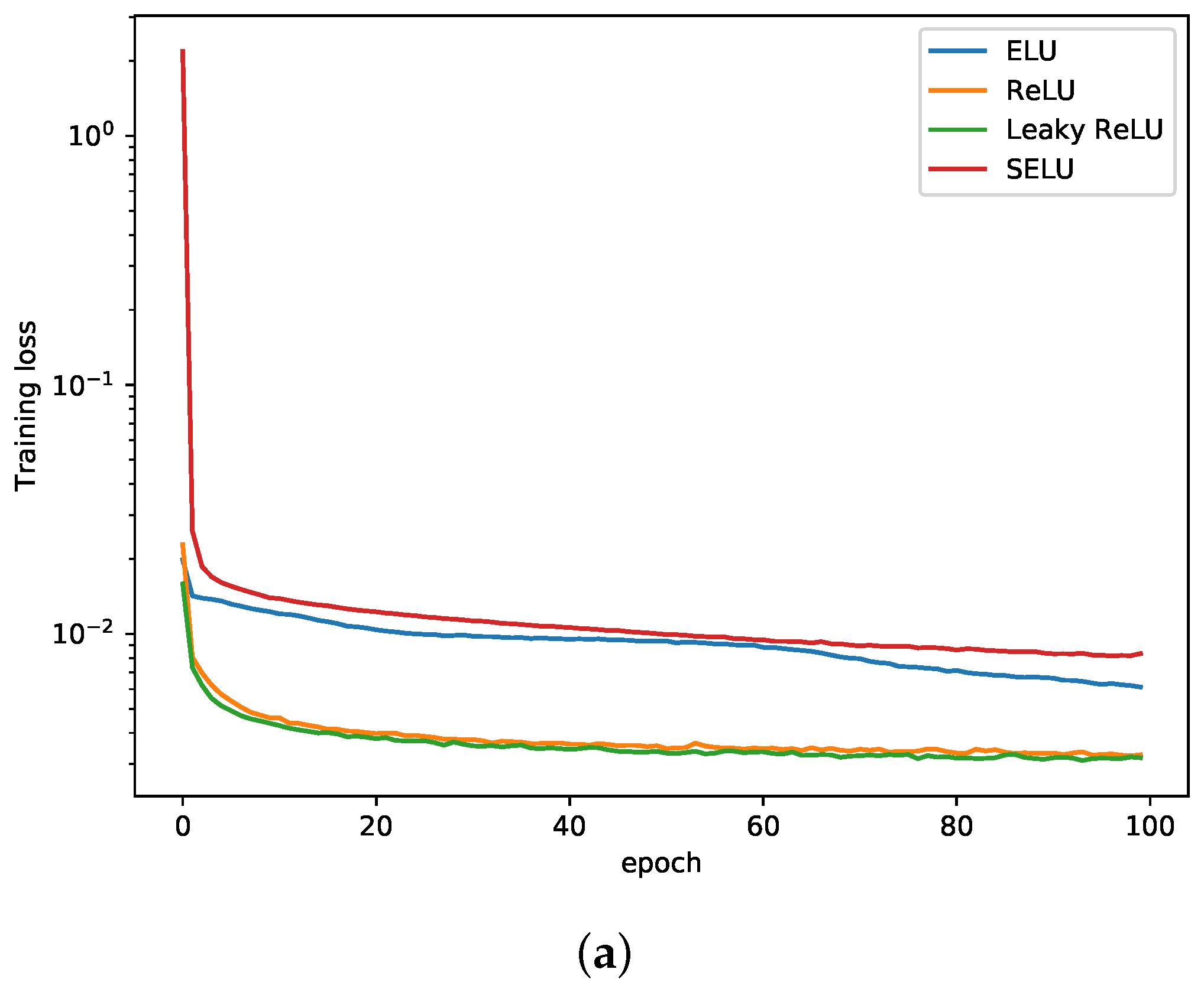
Figure 21.
Comparison of the training loss and validation loss for various activation functions with log scale. Three hidden layers and 512 neurons were used for the 3D-truncated icosahedron tensegrity example. (a) Training loss. (b) Validation loss.
Figure 21.
Comparison of the training loss and validation loss for various activation functions with log scale. Three hidden layers and 512 neurons were used for the 3D-truncated icosahedron tensegrity example. (a) Training loss. (b) Validation loss.
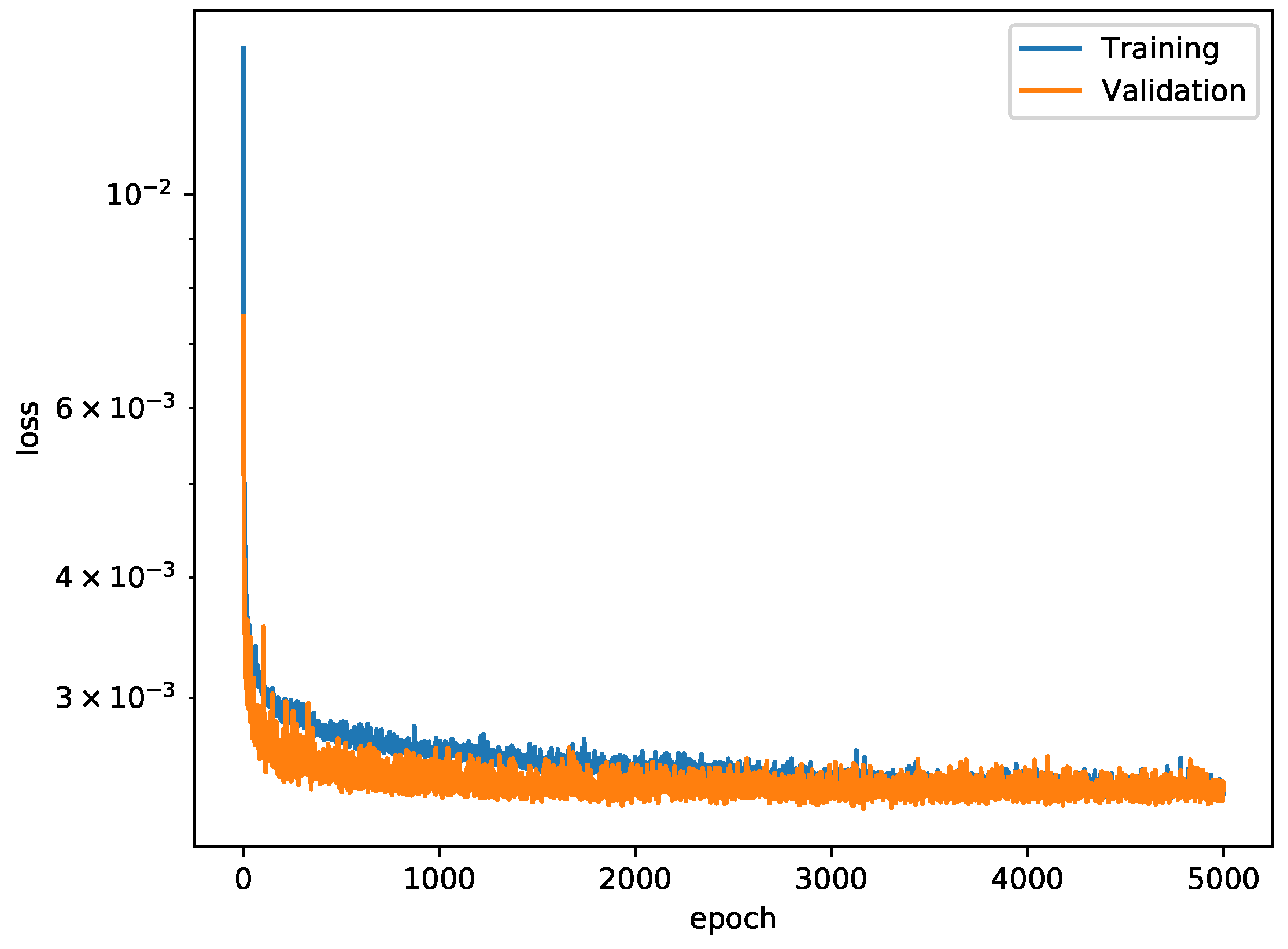
Figure 22.
The training and validation loss curves for the 3D-truncated icosahedron tensegrity.
Figure 22.
The training and validation loss curves for the 3D-truncated icosahedron tensegrity.
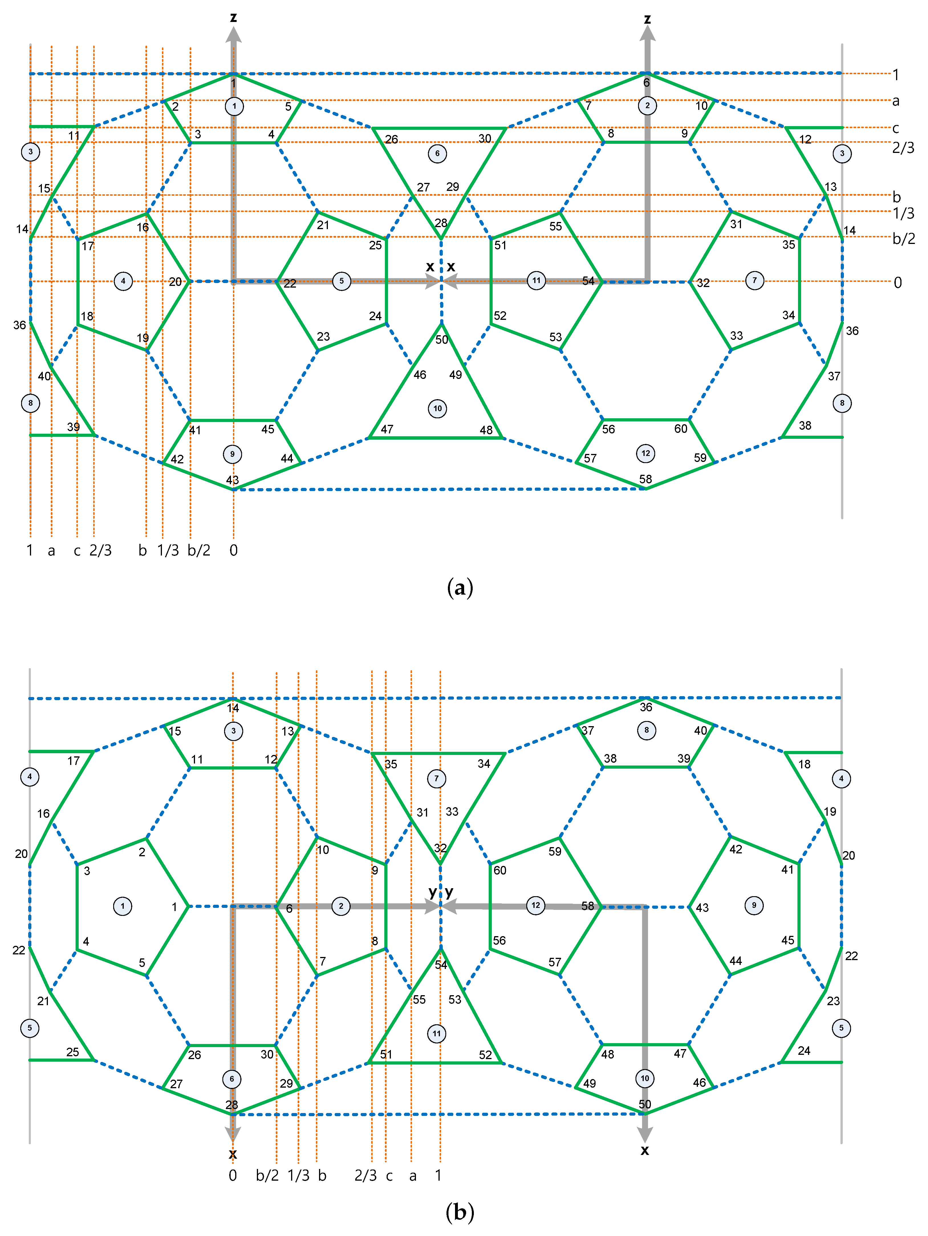
Figure 23.
Rectangular coordinates of the 3D-truncated icosahedron tensegrity in a cube, where , , and . (a) Front view. (b) Top view.
Figure 23.
Rectangular coordinates of the 3D-truncated icosahedron tensegrity in a cube, where , , and . (a) Front view. (b) Top view.
Figure 24.
Comparison of the force densities of the 3D truncated icosahedron tensegrity using FDM, DNN-based form-finding model with DE algorithm and analytical solution [
6].
Figure 24.
Comparison of the force densities of the 3D truncated icosahedron tensegrity using FDM, DNN-based form-finding model with DE algorithm and analytical solution [
6].
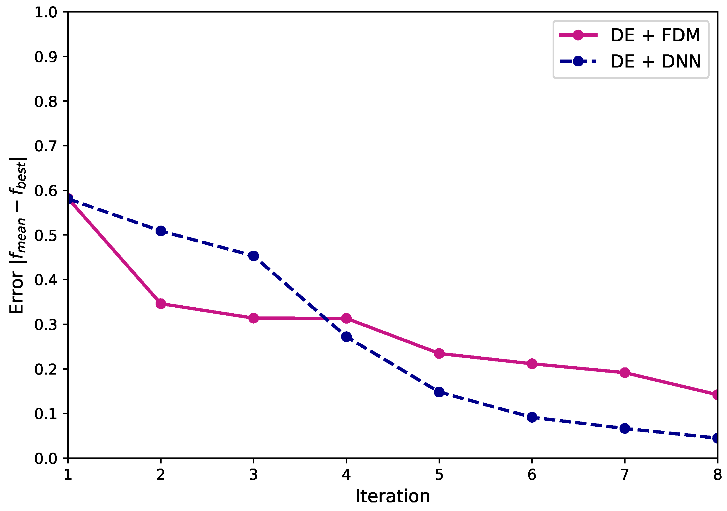
Figure 25.
Relationship between the iteration and error of the 3D truncated icosahedron tensegrity using an FDM and a DNN-based form-finding model with a DE algorithm.
Figure 25.
Relationship between the iteration and error of the 3D truncated icosahedron tensegrity using an FDM and a DNN-based form-finding model with a DE algorithm.
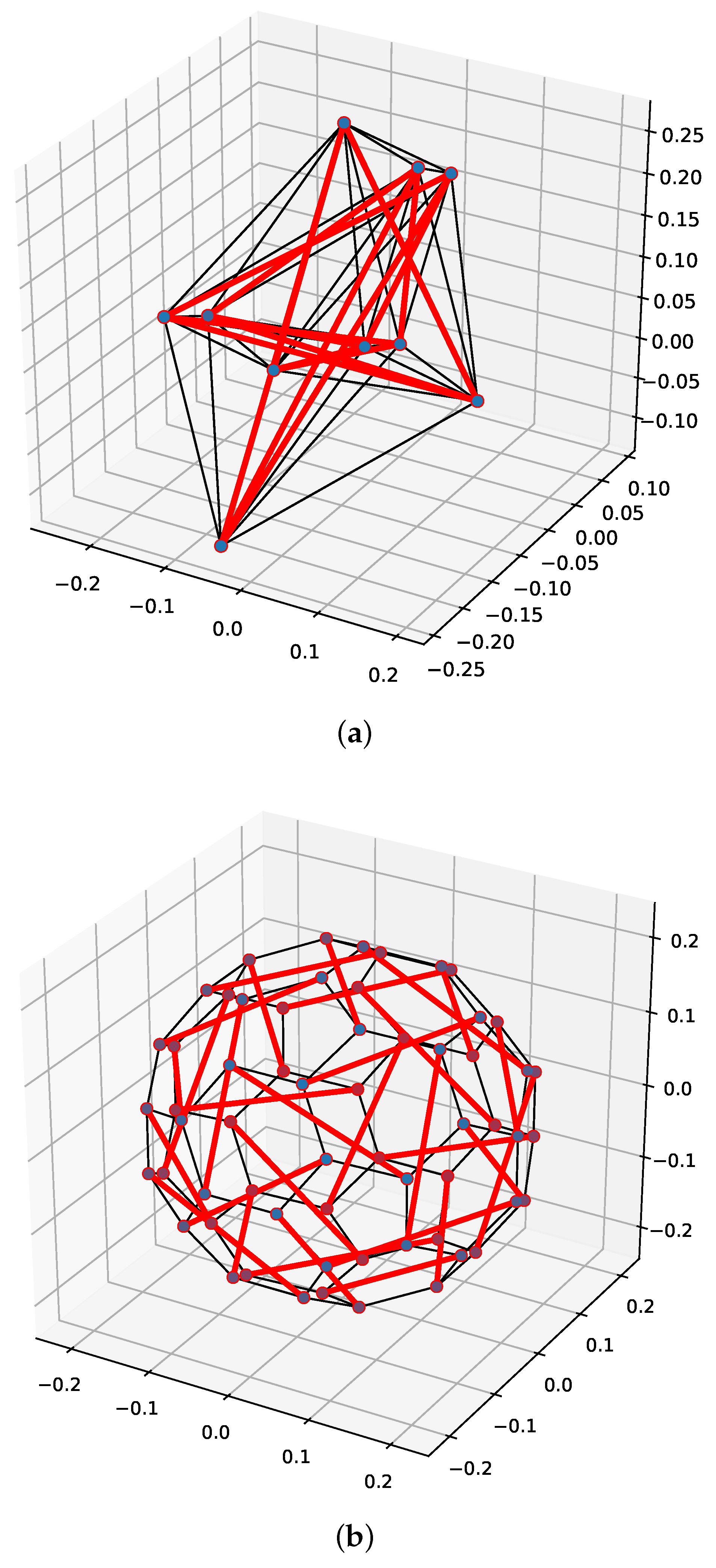
Figure 26.
Final geometry of eight iterations of the 3D-truncated icosahedron tensegrity module using an FDM and a DNN-based form-finding model with DE algorithm. (a) FDM. (b) DNN-based form-finding model.
Figure 26.
Final geometry of eight iterations of the 3D-truncated icosahedron tensegrity module using an FDM and a DNN-based form-finding model with DE algorithm. (a) FDM. (b) DNN-based form-finding model.
Table 1.
The incidence matrix of the 2D two-strut tensegrity structure.
Table 1.
The incidence matrix of the 2D two-strut tensegrity structure.
| Elements | Nodes |
|---|
| 1 | 2 | 3 | 4 |
|---|
| 1 | 1 | −1 | 0 | 0 |
| 2 | 0 | 1 | −1 | 0 |
| 3 | 0 | 0 | 1 | −1 |
| 4 | 1 | 0 | 0 | −1 |
| 5 | 1 | 0 | −1 | 0 |
| 6 | 0 | 1 | 0 | −1 |
Table 2.
The equilibrium matrix of the 2D two-strut tensegrity structure.
Table 2.
The equilibrium matrix of the 2D two-strut tensegrity structure.
| Total Number of Elements (b) |
|---|
| 1 | 2 | 3 | 4 | 5 | 6 |
|---|
| 1 | | 0 | 0 | | | 0 |
| 2 | | 0 | 0 | | | 0 |
| 3 | | | 0 | 0 | 0 | |
| 4 | | | 0 | 0 | 0 | |
| 5 | 0 | | | 0 | | 0 |
| 6 | 0 | | | 0 | | 0 |
| 7 | 0 | 0 | | | 0 | |
| 8 | 0 | 0 | | | 0 | |
Table 3.
Main parameters of DE algorithm.
Table 3.
Main parameters of DE algorithm.
| Parameter | Value |
|---|
| Bounds of variables | |
| Population size | 20 |
| Recombination rate | 0.9 |
| Tolerance | |
Table 4.
The final results of the 2D two-strut tensegrity structure using the FDM and DNN-based form-finding model with the DE algorithm.
Table 4.
The final results of the 2D two-strut tensegrity structure using the FDM and DNN-based form-finding model with the DE algorithm.
| | DE + FDM | DE + DNN | |
|---|
| ∣ f–f ∣ | 0.66 | 0.56 | |
| Solution [cable, strut] | [1.00, −0.97] | [1.00, −1.00] | |
| Force density * [cable, strut] | [1.00, −0.97] | [1.00, −1.00] | [1.00, −1.00] |
Table 5.
The final results of the 3D-truncated tetrahedron tensegrity using an FDM and a DNN-based form-finding model with a DE algorithm.
Table 5.
The final results of the 3D-truncated tetrahedron tensegrity using an FDM and a DNN-based form-finding model with a DE algorithm.
| | DE + FDM | DE + DNN |
|---|
| Iteration | 5 | 5 |
| ∣ f–f ∣ | 0.22 | 0.14 |
| Solution [, , ] | [0.96, 0.70, −0.38] | [1.00, 1.00, −0.58] |
| Force density * [, , ] | [1.00, 0.73, −0.39] | [1.00, 1.00, −0.58] |
Table 6.
Connectivity of the strut members for the 3D-truncated tetrahedron tensegrity.
Table 6.
Connectivity of the strut members for the 3D-truncated tetrahedron tensegrity.
|
Element | i | j | Element | i | j | Element | i | j |
|---|
|
91 | 37 | 58 | 101 | 24 | 26 | 111 | 13 | 40 |
| 92 | 14 | 16 | 102 | 27 | 49 | 112 | 12 | 34 |
| 93 | 2 | 20 | 103 | 23 | 50 | 113 | 33 | 36 |
| 94 | 1 | 15 | 104 | 22 | 44 | 114 | 32 | 59 |
| 95 | 5 | 10 | 105 | 43 | 46 | 115 | 8 | 35 |
| 96 | 6 | 29 | 106 | 42 | 57 | 116 | 9 | 11 |
| 97 | 28 | 55 | 107 | 19 | 21 | 117 | 7 | 54 |
| 98 | 48 | 51 | 108 | 18 | 45 | 118 | 31 | 53 |
| 99 | 4 | 30 | 109 | 38 | 41 | 119 | 47 | 56 |
| 100 | 3 | 25 | 110 | 17 | 39 | 120 | 52 | 60 |
Table 7.
Cartesian coordinates of the 3D-truncated icosahedron tensegrity using the connectivity shown in
Figure 17, where
,
, and
.
Table 7.
Cartesian coordinates of the 3D-truncated icosahedron tensegrity using the connectivity shown in
Figure 17, where
,
, and
.
|
No. | x | y | z | No. | x | y | z |
|---|
|
1 | 0 | −b/2 | 1 | 31 | −b | a | 1/3 |
| 2 | −1/3 | −b | a | 32 | −b/2 | 1 | 0 |
| 3 | −b/2 | −c | 2/3 | 33 | −b | a | −1/3 |
| 4 | b/2 | −c | 2/3 | 34 | −c | 2/3 | −b/2 |
| 5 | 1/3 | −b | a | 35 | −c | 2/3 | b/2 |
| 6 | 0 | b/2 | 1 | 36 | −1 | 0 | −b/2 |
|
7 | 1/3 | b | a | 37 | −a | 1/3 | −b |
| 8 | b/2 | c | 2/3 | 38 | −2/3 | b/2 | −c |
| 9 | −b/2 | c | 2/3 | 39 | −2/3 | −b/2 | −c |
| 10 | −1/3 | b | a | 40 | −a | −1/3 | −b |
| 11 | −2/3 | −b/2 | c | 41 | −b/2 | −c | −2/3 |
| 12 | −2/3 | b/2 | c | 42 | −1/3 | −b | −a |
| 13 | −a | 1/3 | b | 43 | 0 | −b/2 | −1 |
| 14 | −1 | 0 | b/2 | 44 | 1/3 | −b | −a |
| 15 | −a | −1/3 | b | 45 | b/2 | −c | −2/3 |
| 16 | −b | −a | 1/3 | 46 | a | −1/3 | −b |
| 17 | −c | −2/3 | b/2 | 47 | 2/3 | −b/2 | −c |
| 18 | −c | −2/3 | −b/2 | 48 | 2/3 | b/2 | −c |
| 19 | −b | −a | −1/3 | 49 | a | 1/3 | −b |
| 20 | −b/2 | −1 | 0 | 50 | 1 | 0 | −b/2 |
| 21 | b | −a | 1/3 | 51 | c | 2/3 | b/2 |
| 22 | b/2 | −1 | 0 | 52 | c | 2/3 | −b/2 |
| 23 | b | −a | −1/3 | 53 | b | a | −1/3 |
| 24 | c | −2/3 | −b/2 | 54 | b/2 | 1 | 0 |
| 25 | c | −2/3 | b/2 | 55 | b | a | 1/3 |
| 26 | 2/3 | −b/2 | c | 56 | b/2 | c | −2/3 |
| 27 | a | −1/3 | b | 57 | 1/3 | b | −a |
| 28 | 1 | 0 | b/2 | 58 | 0 | b/2 | −1 |
| 29 | a | 1/3 | b | 59 | −1/3 | b | −a |
| 30 | 2/3 | b/2 | c | 60 | −b/2 | c | −2/3 |
Table 8.
The final results of the 3D-truncated icosahedron tensegrity using an FDM and a DNN-based form-finding model with a DE algorithm.
Table 8.
The final results of the 3D-truncated icosahedron tensegrity using an FDM and a DNN-based form-finding model with a DE algorithm.
| | DE + FDM | DE + DNN |
|---|
| Iteration | 8 | 8 |
| ∣ f–f ∣ | 0.14 | 0.04 |
| Solution [, , ] | [1.00, 1.00, −1.00] | [1.00, 0.80, −0.35] |
| Force density * [, , ] | [1.00, 1.00, −1.00] | [1.00, 0.80, −0.35] |


