Accurate Goertzel Algorithm: Error Analysis, Validations and Applications

Abstract

The Horner and Goertzel algorithms are frequently used in polynomial evaluation. Each of them can be less expensive than the other in special cases. In this paper, we present a new compensated algorithm to improve the accuracy of the Goertzel algorithm by using error-free transformations. We derive the forward round-off error bound for our algorithm, which implies that our algorithm yields a full precision accuracy for polynomials that are not too ill-conditioned. A dynamic error estimate in our algorithm is also presented by running round-off error analysis. Moreover, we show the cases in which our algorithms are less expensive than the compensated Horner algorithm for evaluating polynomials. Numerical experiments indicate that our algorithms run faster than the compensated Horner algorithm in those cases while producing the same accurate results, and our algorithm is absolutely stable when the condition number is smaller than ${10}^{16}$. An application is given to illustrate that our algorithm is more accurate than MATLAB’s $\mathtt{fft}$ function. The results show that the relative error of our algorithm is from ${10}^{15}$ to ${10}^{17}$, and that of the $\mathtt{fft}$ was from ${10}^{12}$ to ${10}^{15}$.

1. Introduction

Polynomial evaluation is ubiquitous in computational sciences and their applications, such as interpolation and approximation practices and signal processing. This article will investigate a broader situation of polynomial evaluation:

$$\omega \left(z\right)=\sum _{n=0}^N{a}_n{z}^n,$$

(1)

where $z,a_0,a_1,\dots ,a_N\in \mathbb{C}$. The nested-type algorithms are usually used to evaluate polynomials. The Horner algorithm is the most widely used polynomial evaluation algorithm [1]. In special cases, like $z\in \mathbb{C}$ and $a_0,a_1,\dots ,a_N\in \mathbb{R}$, the Goertzel algorithm that can be applied to compute the discrete Fourier transform (DFT) of specific indices in a vector [2,3] is less expensive the Horner algorithm. The numerical stability of the Horner and Goertzel algorithms was given by Wilkinson [4] and Smoktunowicz [5]. The computed results from these algorithms are arbitrarily less accurate than the working precision u when the polynomial is ill-conditioned due to the round-off errors in floating-point arithmetic. The relative accuracy of these algorithms verifies the following priori bound:

$$\frac{|\omega \left(z\right)-\widehat{\omega }\left(z\right)|}{\left|\omega \right(z\left)\right|}\le \mathtt{cond}(\omega ,z)\times \mathcal{O}\left(u\right),$$

(2)

where $\widehat{\omega }\left(z\right)$ is the computed result and $\mathtt{cond}(\omega ,z)={\sum }_{n=0}^N|a_n{\left|\right|z|}^n/\left|{\sum }_{n=0}^N{a}_n{z}^n\right|$ is the condition number.

In order to improve the accuracy of double precision, Bailey [6] proposed a famous library for double-double and quad-double arithmetic. However, this library needs to normalize floating-point numbers in every operation, and thus the instruction level parallelism is affected [7,8]. The compensated algorithm is improved to solve this problem with the developments and applications of error-free transformation [9]. The relative accuracy of compensated algorithms verifies the following priori bound:

$$\frac{|\omega \left(z\right)-\overline{\omega }\left(z\right)|}{\left|\omega \right(z\left)\right|}\le u+\mathtt{cond}(\omega ,z)\times \mathcal{O}\left(u^2\right),$$

(3)

where $\overline{\omega }\left(z\right)$ is the computed result of a compensated algorithm.

Recently, compensated algorithms have been widely studied in evaluating polynomials. Graillat [10] proposed a compensated Horner algorithm that achieves full precision accuracy for polynomials that are not excessively ill-conditioned. Aside from that, he extended the error-free transformation and compensated Horner algorithm in complex floating-point arithmetic [11,12] and applied a compensated Horner algorithm to evaluate rational functions [13] and solve all polynomial roots [14]. Polynomial series represented in other basis were also considered, such as the Chebyshev form evaluated by a compensated Chenshaw algorithm [15], the Bernstein form evaluated by a compensated de Casteljau algorithm [16], and a compensated Volk and Schumaker(VS) algorithm [17]. Furthermore, the compensated idea is also applied to matrix multiplication to obtain more accurate results [18,19,20].

With the wide application of floating-point numbers and floating-point operations in numerical computing, the analysis of rounding errors has become the focus [21,22]. Running round-off errors are analyzed and applied to many algorithms of polynomial evaluation [23]. Delgado [17] proposed an adaptive evaluation algorithm by using the de Casteljau algorithm and compensated VS algorithms with a dynamic error estimate. Jiang [24] presented running round-off error analysis for evaluating elementary symmetric functions in real and complex floating-point arithmetic. Barrio [25] developed a more complete compensated algorithm library to evaluate orthogonal polynomial series with dynamic error estimates. In addition, error analysis can also be used for machine learning and the numerical solution of differential equations [26].

In this paper, our contributions are as follows:

• We design a new compensated Goertzel algorithm and prove that our algorithm can almost yield full working precision to evaluate polynomials (1);
• We propose dynamic error estimates, which can offer a sharper bound for our approach without considerably increasing its computing complexity;
• Numerical experiments show that our algorithm runs faster than the compensated Horner algorithm in some cases while keeping a similar precision accuracy;
• An application is given to illustrate that our algorithm outperforms MATLAB’s $\mathtt{fft}$ when dealing with the DFT.

The rest of this paper is organized as follows. Section 2 introduces our compensated Goertzel algorithm. A dynamic error estimate is proposed in Section 3. Section 4 analyzes numerical experiment results and gives an application to illustrate that our algorithm outperforms them. Finally, the full paper is summarized in Section 5.

2. Goertzel Compensated Algorithm

We assume working with IEEE-754 floating-point standard [27] rounding to the nearest value in this paper. Let $\mathbb{F}$ be the set of floating-point numbers, $\mathbb{C}$ represent the complex number, and $\{\oplus ,\ominus ,\otimes ,\oslash \}$ represent a floating-point operation. This part presents how to design the Goertzel compensated algorithm. First, the Goertzel algorithm and its relationship with the Clenshaw algorithm are listed. Then, the error-free transformations and sum of squares algorithm are recalled. At last, we present the compensated Goertzel algorithm.

2.1. Goertzel Algorithm

By assuming $\lambda ,z\in \mathbb{C}$ and $z=x+iy$, then we have a quadratic polynomial

$$(\lambda -z)(\lambda -\overline{z})={\lambda }^2-p\lambda +q,$$

(4)

where $p=2x$ and $q={\left|z\right|}^2$. By dividing the polynomial in Equation (1) by that in Equation (4), we obtain

$$\omega \left(\lambda \right)=b_0+b_1\lambda +(\lambda -z)(\lambda -\overline{z})\sum _{n=2}^N{b}_n{\lambda }^{n-2},$$

(5)

where

$$\begin{array}{c}\hfill \left\{\begin{array}{cc}\hfill a_0& =b_0+q{b}_2,\hfill \\ \hfill a_1& =b_1-p{b}_2+q{b}_3,\hfill \\ \hfill ⋮\\ \hfill a_n& =b_n-p{b}_{n+1}+q{b}_{n+2}.\hfill \end{array}\right.\end{array}$$

(6)

Thus, the evaluated result of the polynomial in Equation (1) is

$$\omega \left(z\right)=b_0+b_{1}z.$$

(7)

Above Equations (5)–(7), we can find the Goertzel algorithm [2] with Algorithm 1.

Algorithm 1 Polynomial evaluation by Goertzel algorithm

Function:  $\omega \left(z\right)=\mathtt{Goertzel}({\left(a_n\right)}_{n=0}^N,z)$ Require: $z=x+iy\in \mathbb{C}$, ${\left(a_n\right)}_{n=0}^N\in \mathbb{C}$ Ensure:  $\omega \left(z\right)={\sum }_{n=0}^N{a}_n{z}^n$    $p=2x,q=x^2+y^2$    $b_{N+1}=b_{N+2}=0$    for  $n=N,N-1,...,1$       $b_n=a_n+p{b}_{n+1}-q{b}_{n+2}$    end    $b_0=a_0+x{b}_1-q{b}_2$    $\omega \left(z\right)=b_0+iy{b}_1$

In floating-point arithmetic, a backward error bound for the computed result of the polynomial evaluation by Algorithm 1 is presented by Smoktunowicz [5] as Theorem 1:

Theorem 1.

Assume $z,a_n\in \mathbb{F}+i\mathbb{F}$ for $n=0,\dots ,N$. Let $10N^{2}u\le 0.1$. Then the Goertzel algorithm for evaluating the polynomial in Equation (1) is componentwise backward stable such that

$$\widehat{\omega }\left(z\right)=\sum _{n=0}^N{a}_n(1+{\Delta }_n)z^n,$$

(8)

where

$$|{\Delta }_n|\le 10N^{2}u+\mathcal{O}\left(u^2\right).$$

(9)

In fact, Algorithm 1 is a special case of the Clenshaw algorithm [2,5]. When we let $t=x/\left|z\right|$ and $B_n=b_n{\left|z\right|}^n$, Algorithm 1 can be represented in Clenshaw form [28]:

$$B_n=a_n{\left|z\right|}^n+2t{B}_{n+1}-B_{n+2}.$$

(10)

According to the properties of the Chebyshev polynomial series [29] evaluated by the Clenshaw algorithm, we have

$$\begin{array}{c}\hfill \left\{\begin{array}{cc}\hfill b_n& =\sum _{k=n}^N{a}_k{\left|z\right|}^{k-n}{U}_{k-n}\left(t\right),\hfill \\ \hfill b_0& =\sum _{k=0}^N{a}_k{\left|z\right|}^k{T}_k\left(t\right),\hfill \\ \hfill n& =1,2,\dots ,N.\hfill \end{array}\right.\end{array}$$

(11)

where $T_k\left(t\right)$ and $U_k\left(t\right)$ are Chebyshev polynomials of the first and second kinds, respectively. They satisfy

$$|T_k\left(t\right)|\le 1,|U_k\left(t\right)|\le k+1,$$

(12)

and

$$\frac{z^k}{{\left|z\right|}^k}=T_k\left(t\right)+i\frac{y}{\left|z\right|}{U}_{k-1}\left(t\right)fork=0,1,\dots ,N.$$

(13)

2.2. Error-Free Transformations and Sum of Squares Algorithm

The basic algorithms of error-free transformations are $\mathtt{TwoSum}$ and $\mathtt{TwoProd}$, which were presented by Knuth [30] and Dekker [31], respectively. Graillat [11] extended the addition and multiplication to complex number cases, which are $\mathtt{TwoSumCplx}$ and $\mathtt{TwoProdCplx}$, respectively. In this paper, we shall use a new product error-free transformation of one real and one complex floating-point number, which is called $\mathtt{TwoProdRC}$ in Algorithm 2.

Algorithm 2 Error-free transformation of the product of real and complex floating-point numbers

Function:  $[x,y]=\mathtt{TwoProdRC}(a,b)$ Require: $a\in \mathbb{F}$, $b=c+id\in \mathbb{F}+i\mathbb{F}$ Ensure:   $x+y=a\times b$    $[p,e]=\mathtt{TwoProd}(a,c)$    $[f,g]=\mathtt{TwoProd}(a,d)$    $x=p+if$    $y=e+ig$

The details of the error-free transformations above are presented in Table 1.

Table 1. Error-free transformations, their properties and operation costs.

Algorithm	Properties	Flops
$[\mathtt{x},\mathtt{y}]=\mathtt{TwoSum}(\mathtt{a},\mathtt{b})$	$x=a\oplus b$, $x+y=a+b$	6
$[\mathtt{x},\mathtt{y}]=\mathtt{TwoProd}(\mathtt{a},\mathtt{b})$	$x=a\otimes b$, $x+y=a\times b$	17
$[\mathtt{x},\mathtt{y}]=\mathtt{TwoProdRC}(\mathtt{a},\mathtt{b})$	$x=a\otimes b$, $x+y=a\times b$	34
$[\mathtt{x},\mathtt{y}]=\mathtt{TwoSumCplx}(\mathtt{a},\mathtt{b})$	$x=a\oplus b$, $x+y=a+b$	12
$[\mathtt{p},\mathtt{e},\mathtt{f},\mathtt{g}]=\mathtt{TwoProdCplx}(\mathtt{a},\mathtt{b})$	$p=a\otimes b$, $p+e+f+g=a\times b$	80

{⊕, ⊗} represents {+, ×} in floating-point operations.

Furthermore, the sum of squares algorithm [32] is given in Algorithm 3. It requires 42 flops.

Algorithm 3 Sum of squares by two floating-point numbers

Function:   $[x,y]=\mathtt{SumOfSquares}(a,b)$ Require:  $a,b\in \mathbb{F}$ Ensure:   $x+y\approx a^2+b^2$    $[p,f]=\mathtt{TwoProd}(a,a)$    $[e,g]=\mathtt{TwoProd}(b,b)$    $[x,h]=\mathtt{TwoSum}(p,e)$    $y=f\oplus g\oplus h$

2.3. Compensated Goertzel Algorithm

Although Algorithm 1 is a special Clenshaw algorithm, computation via Equation (10) is more expensive. Thus, using the compensated Clenshaw algorithm [28] to express the compensated Goertzel algorithm is not a good idea. We design a compensated Goertzel algorithm by using $\mathtt{SumOfSquares}$, $\mathtt{TwoSumCplx}$ and $\mathtt{TwoProdRC}$ algorithms to record the round-off errors.

Assume $\widehat{a}\in \mathbb{F}$ is a computed result in floating-point arithmetic, and its perturbation is $ϵa$ such that

$$\widehat{a}=a+ϵa.$$

(14)

$\mathtt{SumOfSquares}$ can find the approximate round-off error $\widehat{ϵq}$ of q. Other round-off errors in Algorithm 1 can be accurately computed by error-free transformation algorithms $\mathtt{TwoSumCplx}$ and $\mathtt{TwoProdRC}$. Then, we can combine all round-off errors by ${\widehat{\ell }}_n$ and find the approximate perturbation ${\widehat{ϵb}}_n$ of $b_n$ for $n=N-1,N-2,\dots ,1$ in each loop. The loop ends using $\mathtt{TwoProdRC}$ and $\mathtt{TwoSumCplx}$ to calculate ${\widehat{b}}_0$ and combines all round-off errors to obtain the approximate perturbation. The round-off error of $y\otimes {\widehat{b}}_1$ should also be considered by $\mathtt{TwoProdRC}$. The compensated Goertzel algorithm is presented in Algorithm 4, and Figure 1 shows the flow chart of this algorithm.

Algorithm 4 Polynomial evaluation by compensated Goertzel algorithm

Function:  $\overline{\omega }\left(z\right)=\mathtt{CompGoertzel}({\left(a_n\right)}_{n=0}^N,z)$ Require: $z=x+iy\in \mathbb{F}+i\mathbb{F}$, ${\left(a_n\right)}_{n=0}^N\in \mathbb{F}+i\mathbb{F}$ Ensure:  $\overline{\omega }\left(z\right)\approx {\sum }_{n=0}^N{a}_n{z}^n$    $p=2x$    $[\widehat{q},\widehat{ϵq}]=\mathtt{SumOfSquares}(x,y)$    ${\widehat{b}}_N=a_N,{\widehat{b}}_{N+1}={\widehat{ϵb}}_N={\widehat{ϵb}}_{N+1}=0$    for  $n=N-1,N-2...,1$       $[r_n,{\pi }_n]=\mathtt{TwoProdRC}(p,{\widehat{b}}_{n+1})$       $[s_n,{\sigma }_n]=\mathtt{TwoProdRC}(-\widehat{q},{\widehat{b}}_{n+2})$       $[t_n,{\eta }_n]=\mathtt{TwoSumCplx}(r_n,s_n)$       $[{\widehat{b}}_n,{\xi }_n]=\mathtt{TwoSumCplx}(t_n,a_n)$       ${\widehat{\ell }}_n={\pi }_n\oplus {\sigma }_n\oplus {\eta }_n\oplus {\xi }_n\ominus \widehat{ϵq}\otimes {\widehat{b}}_{n+2}$       ${\widehat{ϵb}}_n={\widehat{\ell }}_n\oplus p\otimes {\widehat{ϵb}}_{n+1}\ominus \widehat{q}\otimes {\widehat{ϵb}}_{n+2}$    end    $[r_0,{\pi }_0]=\mathtt{TwoProdRC}(x,{\widehat{b}}_1)$    $[s_0,{\sigma }_0]=\mathtt{TwoProdRC}(-\widehat{q},{\widehat{b}}_2)$    $[t_0,{\eta }_0]=\mathtt{TwoSumCplx}(r_0,s_0)$    $[{\widehat{b}}_0,{\xi }_0]=\mathtt{TwoSumCplx}(t_0,a_0)$    ${\widehat{\ell }}_0={\pi }_0\oplus {\sigma }_0\oplus {\eta }_0\oplus {\xi }_0\ominus \widehat{ϵq}\otimes {\widehat{b}}_2$    ${\widehat{ϵb}}_0={\widehat{\ell }}_0\oplus x\otimes {\widehat{ϵb}}_1\ominus \widehat{q}\otimes {\widehat{ϵb}}_2$    $\left[\varphi ,\psi \right]=\mathtt{TwoProdRC}(y,{\widehat{b}}_1)$    $\widehat{e}={\widehat{ϵb}}_0\oplus i({\widehat{ϵb}}_1\otimes y\oplus \psi )$    $\widehat{\omega }\left(z\right)={\widehat{b}}_0\oplus i\varphi$    $\overline{\omega }\left(z\right)=\widehat{\omega }\left(z\right)\oplus \widehat{e}$

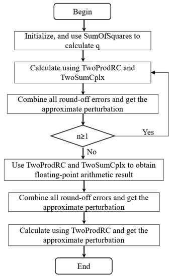
Figure 1. The flowchart of the compensated Goertzel algorithm.

We remark that if ${\left(a_n\right)}_{n=0}^N\in \mathbb{F}$, then we shall replace $\mathtt{TwoSumCplx}$ and $\mathtt{TwoProdRC}$ with $\mathtt{TwoSum}$ and $\mathtt{TwoProd}$ in Algorithm 4, respectively.

3. Round-Off Error and Complexity Analysis

In this section, we consider the error bound and complexity of Algorithm 4 through Higham’s theories [33]. In our analysis, we assume that there is no computational overflow or underflow. First, we present the priori bound by forward round-off error analysis. Then, we show a dynamic error estimate by running round-off error analysis. At last, we compare the complexities of Horner, Goertzel, their compensated algorithms and the compensated Goertzel algorithm with a dynamic error estimate to evaluate the polynomial in Equation (1) in real and complex coefficients.

3.1. Forward Round-Off Error Analysis

Let ⧫ $\in \{\oplus ,\ominus ,\otimes ,\oslash \}$, $\circ \in \{+,-,\times ,÷\}$ and $a,b\in \mathbb{F}$. Then, a floating-point computation obeys the model

$$a⧫b=(a\circ b)(1+{\epsilon }_1)=\frac{a\circ b}{1+{\epsilon }_2},$$

(15)

where $|{\epsilon }_1|,|{\epsilon }_2|\le u$. We define

$$<N>:=1+{\theta }_N=\prod _{n=1}^N{(1+{\epsilon }_n)}^{{\rho }_n},$$

(16)

where $|{\epsilon }_n|\le u,{\rho }_n=\pm 1$ and

$$|{\theta }_n|\le {\gamma }_n:=\frac{nu}{(1-nu)},$$

(17)

for $n=1,2,\dots ,N$ and $Nu<1$. We assume that $\widehat{a}$ and $\widehat{b}$ in real arithmetic are denoted by $\tilde{c}=\widehat{a}\circ \widehat{b}$, which will be used in our later analysis.

Lemma 1 summarizes the properties of the error-free transformations in Table 1:

Lemma 1.

For $a,b,x,y\in \mathbb{F}$, $[x,y]=\mathtt{TwoSum}(a,b)$ verifies

$$\left|y\right|\le u\left|x\right|,\left|y\right|\le u|a+b|,$$

(18)

In addition, $[x,y]=\mathtt{TwoProd}(a,b)$ verifies

$$\left|y\right|\le u\left|x\right|,\left|y\right|\le u|a\times b|.$$

(19)

For $a,b,x,y\in \mathbb{F}+i\mathbb{F}$, $[x,y]=\mathtt{TwoSumCplx}(a,b)$ verifies

$$\left|y\right|\le u\left|x\right|,\left|y\right|\le u|a+b|,$$

(20)

Additionally, $[x,y]=\mathtt{TwoProdRC}(a,b)$ verifies

$$\left|y\right|\le u\left|x\right|,\left|y\right|\le u|a\times b|.$$

(21)

For $a,b,p,e,f,g\in \mathbb{F}+i\mathbb{F}$, $[p,e,f,g]=\mathtt{TwoProdCplx}(a,b)$ verifies

$$|e+f+g|\le \sqrt{2}{\gamma }_2|a\times b|.$$

(22)

Proof. 

Equations (18)–(22) are presented in [9,11]. In Algorithm 2, it is easy to obtain Equation (21) from Equation (18).    □

Lemma 2 shows the property of Algorithm 3:

Lemma 2.

For $a,b,x,y\in \mathbb{F}$, $[x,y]=\mathtt{SumOfSquares}(a,b)$ verifies

$$\begin{array}{c}\hfill \begin{array}{cc}& \left|x\right|\le (1+{\gamma }_2)|a^2+b^2|,\hfill \\ & \left|y\right|\le {\gamma }_2\left|x\right|,\hfill \\ & |x+y-(a^2+b^2)|\le u{\gamma }_3|a^2+b^2|.\hfill \end{array}\end{array}$$

(23)

Proof. 

According to Algorithm 3 and Table 1, $x=a\otimes a\oplus b\otimes b$. With Lemma 1, we obtain $\left|f\right|\le u\left|p\right|,\left|g\right|\le u\left|e\right|$ and $\left|h\right|\le u\left|x\right|$. From Equations (15)–(17), we have

$$\begin{array}{c}\hfill \begin{array}{cc}\hfill \left|x\right|& =|a^2<2>+b^2<2>|\le (1+{\gamma }_2)|a^2+b^2|,\hfill \\ \hfill \left|y\right|& =|f<1>+g<2>+h<1>|\le (1+{\gamma }_2)\left(\right|f|+\left|g\right|+\left|h\right|)\hfill \\ & \le u(1+{\gamma }_2)\left(\right|p|+\left|e\right|+\left|x\right|)\le 2u(1+{\gamma }_2)\left|x\right|={\gamma }_2\left|x\right|.\hfill \end{array}\end{array}$$

(24)

From Theorem 4.2 in [32], $|x+y-(a^2+b^2)|\le \frac{3u^2}{1-3u^2}|a^2+b^2|\le u{\gamma }_3|a^2+b^2|$.    □

Theorem 2 presents a priori error bound of Algorithm 4 to evaluate the polynomial in Equation (1) in complex floating-point arithmetic.

Theorem 2.

Assume $z,a_n\in \mathbb{F}+i\mathbb{F}$ for $n=0,\dots ,N$. Then, the relative forward round-off error bound in the compensated Goertzel algorithm for evaluting $\omega \left(z\right)={\sum }_{n=0}^N{a}_n{z}^n$ in floating-point arithmetic satisfies

$$\begin{array}{c}\hfill \frac{|\mathtt{CompGoertzel}({\left(a_n\right)}_{n=0}^N,z)-\omega \left(z\right)|}{\left|\omega \right(z\left)\right|}\le u+3N^2{\gamma }_{15}{\gamma }_{3N+1}\mathtt{cond}(\omega ,z).\end{array}$$

(25)

Proof. 

Assume the error of $\widehat{\omega }\left(z\right)$ is e (i.e., $\widehat{\omega }\left(z\right)+e=\omega \left(z\right)$). Then, we have

$$\begin{array}{c}\hfill \begin{array}{cc}\hfill |\overline{\omega }\left(z\right)-\omega \left(z\right)|& =|(\widehat{\omega }\left(z\right)\oplus \widehat{e})-\omega \left(z\right)|=|(1+\epsilon )(\widehat{\omega }\left(z\right)+\widehat{e})-\omega \left(z\right)|\hfill \\ & =|(1+\epsilon )(\omega \left(z\right)-e+\widehat{e})-\omega \left(z\right)|\le u|\omega \left(z\right)|+(1+u)|e-\widehat{e}|,\hfill \end{array}\end{array}$$

(26)

and

$$e={ϵb}_0+i({ϵb}_{1}y+\psi ),$$

(27)

where ${ϵb}_0$ and ${ϵb}_1$ are the error of $b_0$ and $b_1$, respectively, such that

$$\begin{array}{c}\hfill \begin{array}{cc}\hfill {ϵb}_n& ={\ell }_n+p{ϵb}_{n+1}+q{ϵb}_{n+2},\hfill \\ \hfill {ϵb}_0& ={\ell }_0+x{ϵb}_1+q{ϵb}_2,\hfill \end{array}\end{array}$$

(28)

where ${\ell }_n={\pi }_n+{\sigma }_n+{\eta }_n+{\xi }_n-ϵq{b}_{n+2}$ for $n=N-1,N-2\dots ,0$. Similarly, let

$$\begin{array}{c}\hfill \begin{array}{cc}\hfill \tilde{e}& ={\widetilde{ϵb}}_0+i({\widetilde{ϵb}}_{1}y+\psi ),\hfill \\ \hfill \widehat{e}& ={\widehat{ϵb}}_0\oplus i({\widehat{ϵb}}_1\otimes y\oplus \psi ),\hfill \end{array}\end{array}$$

(29)

where

$$\begin{array}{c}\hfill \begin{array}{cc}\hfill {\widetilde{ϵb}}_n& ={\widehat{\ell }}_n+p{\widetilde{ϵb}}_{n+1}+\widehat{q}{\widetilde{ϵb}}_{n+2},\hfill \\ \hfill {\widetilde{ϵb}}_0& ={\widehat{\ell }}_0+x{\widetilde{ϵb}}_1+\widehat{q}{\widetilde{ϵb}}_2,\hfill \end{array}\end{array}$$

(30)

and

$$\begin{array}{c}\hfill \begin{array}{cc}\hfill {\widehat{ϵb}}_n& ={\widehat{\ell }}_n\oplus p\otimes {\widehat{ϵb}}_{n+1}\oplus \widehat{q}\otimes {\widehat{ϵb}}_{n+2},\hfill \\ \hfill {\widehat{ϵb}}_0& ={\widehat{\ell }}_0\oplus x\otimes {\widehat{ϵb}}_1\oplus \widehat{q}\otimes {\widehat{ϵb}}_2,\hfill \end{array}\end{array}$$

(31)

where ${\widehat{\ell }}_n={\pi }_n\oplus {\sigma }_n\oplus {\eta }_n\oplus {\xi }_n\ominus \widehat{ϵ}q\otimes {\widehat{b}}_{n+2}$ for $n=N-1,N-2\dots ,0$. Then, Equation (26) can be simplified as

$$|\overline{\omega }\left(z\right)-\omega \left(z\right)|\le u|\omega \left(z\right)|+(1+u)(|e-\tilde{e}|+|\tilde{e}-\widehat{e}\left|\right).$$

(32)

First, we consider the bound of $|e-\tilde{e}|$. From Equations (11), (28) and (30), we have

$$\begin{array}{c}\hfill \begin{array}{cc}\hfill ϵb_1& =\sum _{n=1}^N{\ell }_n{\left|z\right|}^{n-1}{U}_{n-1}\left(t\right),\hfill \\ \hfill ϵb_0& =\sum _{n=0}^N{\ell }_n{\left|z\right|}^n{T}_n\left(t\right),\hfill \\ \hfill {\widetilde{ϵb}}_1& =\sum _{n=1}^N{\widehat{\ell }}_n{\left|z\right|}^{n-1}{U}_{n-1}\left(t\right),\hfill \\ \hfill {\widetilde{ϵb}}_0& =\sum _{n=0}^N{\widehat{\ell }}_n{\left|z\right|}^n{T}_n\left(t\right).\hfill \end{array}\end{array}$$

(33)

Then, by Equations (13), (27) and (29), we deduce

$$\begin{array}{c}\hfill |e-\tilde{e}|=|(ϵb_0-{\widetilde{ϵb}}_0)+i(ϵb_1-{\widetilde{ϵb}}_1)y|=|\sum _{n=0}^{N-1}({\ell }_n-{\widehat{\ell }}_n)z^n|\le \sum _{n=0}^{N-1}|{\ell }_n-{\widehat{\ell }}_n{\left|\right|z|}^n.\end{array}$$

(34)

In Algorithm 4, according to Lemmas 1 and 2, we obtain

$$\begin{array}{c}\hfill \begin{array}{cc}\hfill |{\pi }_n|& \le u|p{\widehat{b}}_{n+1}|\le 2u|z\left|\right|{\widehat{b}}_{n+1}|,\hfill \\ \hfill |{\sigma }_n|& \le u|\widehat{q}{\widehat{b}}_{n+2}|\le u(1+{\gamma }_2){\left|z\right|}^2\left|{\widehat{b}}_{n+2}\right|,\hfill \\ \hfill |{\eta }_n|& \le u|p{\widehat{b}}_{n+1}-\widehat{q}{\widehat{b}}_{n+2}|\le u(1+{\gamma }_2)\left(2\right|z\left|\right|{\widehat{b}}_{n+1}{|+|z|}^2|{\widehat{b}}_{n+2}\left|\right),\hfill \\ \hfill |{\xi }_n|& \le u|a_n+p{\widehat{b}}_{n+1}-\widehat{q}{\widehat{b}}_{n+2}|\le u(1+{\gamma }_2)\left(\right|a_n|+2|z\left|\right|{\widehat{b}}_{n+1}{|+|z|}^2|{\widehat{b}}_{n+2}\left|\right),\hfill \\ \hfill |\widehat{ϵq}|& \le {\gamma }_2|\widehat{q}|\le {\gamma }_2(1+{\gamma }_2){\left|z\right|}^2,\hfill \end{array}\end{array}$$

(35)

for $n=0,1,\dots ,N$, and then

$$\begin{array}{c}\hfill \begin{array}{cc}& |{\pi }_n|+|{\sigma }_n|+|{\eta }_n|+|{\xi }_n|+|\widehat{ϵq}\left|\right|{\widehat{b}}_{n+2}|\hfill \\ \hfill \le & (3u+{\gamma }_2)(1+{\gamma }_2)\left(\right|a_n|+2|z\left|\right|{\widehat{b}}_{n+1}{|+|z|}^2|{\widehat{b}}_{n+2}\left|\right).\hfill \end{array}\end{array}$$

(36)

In Algorithm 4, from Equations (15)–(17), we have

$$\begin{array}{c}\hfill \left\{\begin{array}{cc}\hfill {\widehat{b}}_{N-1}& =p{a}_N<2>+a_{N-1}<1>,\hfill \\ \hfill {\widehat{b}}_{N-2}& =p{\widehat{b}}_{N-1}<3>-q{a}_N<5>+a_{N-2}<1>\hfill \\ & =a_N(p^2-q)<5>+p{a}_{N-1}<3>+a_{N-2}<1>,\hfill \\ \hfill ⋮\\ \hfill {\widehat{b}}_1& =p{\widehat{b}}_2<3>-q{\widehat{b}}_3<5>+a_1<1>\hfill \\ & =a_N(p^{N-1}+\cdots )<3N-4>+a_{N-1}(p^{N-2}+\cdots )<3N-5>+\cdots ,\hfill \\ \hfill {\widehat{b}}_0& =x{\widehat{b}}_1<3>-\widehat{q}{\widehat{b}}_2<5>+a_0<1>\hfill \\ & =a_N(p^N+\cdots )<3N-1>+a_{N-1}(p^{N-1}+\cdots )<3N-2>+\cdots ,\hfill \end{array}\right.\end{array}$$

(37)

Then, by induction, we get

$$|b_n-{\widehat{b}}_n|\le {\gamma }_{3(N-n)-1}\left|b_n\right|,$$

(38)

and

$$|{\widehat{b}}_n|\le (1+{\gamma }_{3(N-n)-1})\left|b_n\right|.$$

(39)

Assume that

$$g_k=\sum _{n=k}^N|a_n{\left|\right|z|}^{n-k},k=0,1,\dots ,N,$$

(40)

Given this, then

$$\sum _{n=0}^N{g}_n{\left|z\right|}^n\le (N+1)g_0.$$

(41)

By combining Equations (11), (12) and (40), we have

$$\begin{array}{c}\hfill \begin{array}{cc}\hfill |b_n|& \le (N-n+1)g_n,n=1,\dots ,N.\hfill \\ \hfill |b_0|& \le g_0.\hfill \end{array}\end{array}$$

(42)

It is easy to obtain that

$${\widehat{\ell }}_n={\pi }_n<4>+{\sigma }_n<4>+{\eta }_n<3>+{\xi }_n<2>-\widehat{ϵ}q{\widehat{b}}_{n+2}<2>,$$

Through Lemma 2 and Equations (36)–(42), we deduce

$$\begin{array}{c}\hfill \begin{array}{cc}& |{\ell }_n-{\widehat{\ell }}_n|\le {\gamma }_4\left(\right|{\pi }_n|+|{\sigma }_n|+|{\eta }_n|+|{\xi }_n|+|\widehat{ϵq}\left|\right|{\widehat{b}}_{n+2}\left|\right)+|ϵq{b}_{n+2}-\widehat{ϵq}{\widehat{b}}_{n+2}|\hfill \\ \hfill \le & {\gamma }_4(3u+{\gamma }_2)(1+{\gamma }_2)\left(\right|a_n|+2|z\left|\right|{\widehat{b}}_{n+1}{|+|z|}^2|{\widehat{b}}_{n+2}\left|\right)+\left|ϵq\right||b_{n+2}-{\widehat{b}}_{n+2}|\hfill \\ & +|ϵq-\widehat{ϵq}\left|\right|{\widehat{b}}_{n+2}|\hfill \\ \hfill \le & {\gamma }_4{\gamma }_5\left(\right|a_n|+2|z\left|\right|{\widehat{b}}_{n+1}{|+|z|}^2|{\widehat{b}}_{n+2}\left|\right)+{\gamma }_2{\gamma }_{3(N-n)-7}{\left|z\right|}^2|b_{n+2}|+u{\gamma }_3{\left|z\right|}^2\left|{\widehat{b}}_{n+2}\right|\hfill \\ \hfill \le & [{\gamma }_5^2(1+{\gamma }_{3(N-n)-4})+{\gamma }_2{\gamma }_{3(N-n)-7}]\left(\right|a_n|+2|z\left|\right|b_{n+1}{|+|z|}^2|b_{n+2}\left|\right)\hfill \\ \hfill \le & {\gamma }_5{\gamma }_{3(N-n)+1}\left(\right|a_n|+2|z\left|\right|b_{n+1}{|+|z|}^2|b_{n+2}\left|\right)\hfill \\ \hfill \le & {\gamma }_5{\gamma }_{3(N-n)+1}\left(\right|a_n|+2(N-n)|z|g_{n+1}+{(N-n-1)\left|z\right|}^2{g}_{n+2})\hfill \\ \hfill \le & 3{\gamma }_5{\gamma }_{3(N-n)+1}(N-n)g_n.\hfill \end{array}\end{array}$$

(43)

Thus, from Equations (34), (41) and (43), we obtain

$$|e-\tilde{e}|\le \sum _{n=0}^{N-1}|{\ell }_n-{\widehat{\ell }}_n{\left|\right|z|}^n\le 3N^2{\gamma }_5{\gamma }_{3N+1}{g}_0.$$

(44)

Second, we consider the bound of $|\tilde{e}-\widehat{e}|$. In Algorithm 4, according to Equations (15)–(17), we have

$$\begin{array}{c}\hfill \left\{\begin{array}{cc}\hfill {\widehat{ϵb}}_{N-1}& ={\widehat{\ell }}_{N-1},\hfill \\ \hfill {\widehat{ϵb}}_{N-2}& =p{\widehat{\ell }}_{N-1}<2>+{\widehat{\ell }}_{N-2}<1>,\hfill \\ \hfill {\widehat{ϵb}}_{N-3}& =p{\widehat{ϵb}}_{N-2}<3>-\widehat{q}{\widehat{\ell }}_{N-1}<3>+{\widehat{\ell }}_{N-3}<1>\hfill \\ & ={\widehat{\ell }}_{N-1}(p^2-\widehat{q})<5>+p{\widehat{\ell }}_{N-2}<3>+{\widehat{\ell }}_{N-3}<1>,\hfill \\ \hfill ⋮\\ \hfill {\widehat{ϵb}}_1& =p{\widehat{ϵb}}_2<3>-\widehat{q}{\widehat{ϵb}}_3<3>+{\widehat{\ell }}_1<1>\hfill \\ & ={\widehat{\ell }}_{N-1}(p^{N-2}+\cdots )<3N-7>+{\widehat{\ell }}_{N-2}(p^{N-3}+\cdots )<3N-8>+\cdots ,\hfill \\ \hfill {\widehat{ϵb}}_0& =x{\widehat{ϵb}}_1<3>-\widehat{q}{\widehat{ϵb}}_2<3>+{\widehat{\ell }}_0<1>\hfill \\ & ={\widehat{\ell }}_{N-1}(p^{N-1}+\cdots )<3N-4>+{\widehat{\ell }}_{N-2}(p^{N-2}+\cdots )<3N-5>+\cdots .\hfill \end{array}\right.\end{array}$$

(45)

Then, by induction, from Equations (13) and (33) as well as Lemma 1, we deduce

$$\begin{array}{c}\hfill |({\widetilde{ϵb}}_0-{\widehat{ϵb}}_0)+i({\widetilde{ϵb}}_1-{\widehat{ϵb}}_1)y|\le {\gamma }_{3N-4}|\sum _{n=0}^{N-1}{\widehat{\ell }}_n{z}^n|\le {\gamma }_{3N-4}\sum _{n=0}^{N-1}|{\widehat{\ell }}_n{\left|\right|z|}^n,\end{array}$$

(46)

and

$$\begin{array}{c}\hfill \begin{array}{cc}\hfill |{\widehat{ϵb}}_0+i({\widehat{ϵb}}_{1}y+\psi )|\le & |{\widehat{ϵb}}_0+i{\widehat{ϵb}}_{1}y|+|\psi |\hfill \\ \hfill \le & (1+{\gamma }_{3N-4})|\sum _{n=0}^{N-1}{\widehat{\ell }}_n{z}^n|+u|y{\widehat{b}}_1|\hfill \\ \hfill \le & (1+{\gamma }_{3N-4})\sum _{n=0}^{N-1}|{\widehat{\ell }}_n{\left|\right|z|}^n+u\left|z\right||{\widehat{b}}_1|.\hfill \end{array}\end{array}$$

(47)

Thus, through Equations (29), (30), (46) and (47), we obtain

$$\begin{array}{c}\hfill \begin{array}{cc}\hfill |\tilde{e}-\widehat{e}|=& |{\widetilde{ϵb}}_0+i({\widetilde{ϵb}}_{1}y+\psi )-{\widehat{ϵb}}_0<2>-i({\widehat{ϵb}}_{1}y+\psi )<3>|\hfill \\ \hfill \le & |({\widetilde{ϵb}}_0-{\widehat{ϵb}}_0)+i({\widetilde{ϵb}}_1-{\widehat{ϵb}}_1)y|+{\gamma }_3|{\widehat{ϵb}}_0+i({\widehat{ϵb}}_{1}y+\psi )|\hfill \\ \hfill \le & {\gamma }_{3N-1}\sum _{n=0}^{N-1}|{\widehat{\ell }}_n{\left|\right|z|}^n+u{\gamma }_3\left|z\right||{\widehat{b}}_1|.\hfill \end{array}\end{array}$$

(48)

According to Equations (36), (39) and (42), we get

$$\begin{array}{c}\hfill \begin{array}{cc}\hfill |{\widehat{\ell }}_n|\le & (1+{\gamma }_5)\left(\right|{\pi }_n|+|{\sigma }_n|+|{\eta }_n|+|{\xi }_n|+|\widehat{ϵ}q\left|\right|{\widehat{b}}_{n+2}\left|\right)\hfill \\ \hfill \le & {\gamma }_9\left(\right|a_n|+2|z\left|\right|{\widehat{b}}_{n+1}{|+|z|}^2|{\widehat{b}}_{n+2}\left|\right)\hfill \\ \hfill \le & {\gamma }_9(1+{\gamma }_{3(N-n)-4})\left(\right|a_n|+2|z\left|\right|b_{n+1}{|+|z|}^2|b_{n+2}\left|\right)\hfill \\ \hfill \le & {\gamma }_9(1+{\gamma }_{3(N-n)-4})\left(\right|a_n|+2(N-n)\left|z\right|g_{n+1}+(N-n-1){\left|z\right|}^2{g}_{n+2})\hfill \\ \hfill \le & 3{\gamma }_9(1+{\gamma }_{3(N-n)-4})(N-n)g_n.\hfill \end{array}\end{array}$$

(49)

Then, by Equations (39), (41), (48) and (49), we obtain

$$\begin{array}{c}\hfill \begin{array}{cc}\hfill |\tilde{e}-\widehat{e}|\le & 3{\gamma }_9{\gamma }_{3N-1}\sum _{n=0}^{N-1}(1+{\gamma }_{3(N-n)-4})(N-n)g_n+u{\gamma }_3(1+{\gamma }_{3N-4})N\left|z\right|g_1\hfill \\ \hfill \le & (1+{\gamma }_{3N-4})N(3N{\gamma }_9{\gamma }_{3N-1}+u{\gamma }_3)g_0\hfill \\ \hfill \le & 3N^2{\gamma }_{10}{\gamma }_{3N-1}{g}_0.\hfill \end{array}\end{array}$$

(50)

Hence, when combining Equations (32), (44) and (50), we have

$$\begin{array}{c}\hfill \begin{array}{cc}\hfill |\overline{\omega }\left(z\right)-\omega \left(z\right)|\le & u\left|\omega \left(z\right)\right|+(1+u)3N^2({\gamma }_5{\gamma }_{3N+1}+{\gamma }_{10}{\gamma }_{3N-1})g_0\hfill \\ \hfill \le & u\left|\omega \left(z\right)\right|+3N^2{\gamma }_{15}{\gamma }_{3N+1}{g}_0.\hfill \end{array}\end{array}$$

(51)

Thus, with $\mathtt{cond}(\omega ,z)=g_0/\left|\omega \left(z\right)\right|$, we deduce Equation (25).    □

3.2. Running Round-Off Error Analysis

Theorem 3 gives a running error bound of Algorithm 4 to evaluate the polynomial in Equation (1) in complex floating-point arithmetic:

Theorem 3.

Assume $z,a_n\in \mathbb{F}+i\mathbb{F}$ for $n=0,\dots ,N$. Then, the running round-off error bound in the compensated Goertzel algorithm for evaluting $\omega \left(z\right)={\sum }_{n=0}^N{a}_n{z}^n$ in floating-point arithmetic satisfies

$$|\overline{\omega }\left(z\right)-\omega \left(z\right)|\le (\left|c\right|\oplus \widehat{\alpha })\oslash (1\ominus 2u),$$

(52)

where

$$\begin{array}{c}\hfill \left\{\begin{array}{cc}\hfill c& =\widehat{\omega }\left(z\right)\oplus \widehat{e}\ominus \overline{\omega }\left(z\right),\hfill \\ \hfill \widehat{\alpha }& ={\widehat{\gamma }}_{3N+1}\otimes \widehat{E}\oslash (1\ominus 6(N-1)\otimes u),\hfill \\ \hfill \widehat{E}& ={\widehat{Eb}}_0\oplus i{\widehat{Eb}}_1\otimes \left|y\right|,\hfill \\ \hfill {\widehat{Eb}}_n& =|\widehat{{\ell }_n}|\oplus \left|p\right|\otimes {\widehat{Eb}}_{n+1}\oplus \left|\widehat{q}\right|\otimes {\widehat{Eb}}_{n+2},\hfill \\ \hfill {\widehat{Eb}}_0& =|\widehat{{\ell }_0}|\oplus \left|x\right|\otimes {\widehat{Eb}}_1\oplus \left|\widehat{q}\right|\otimes {\widehat{Eb}}_2,\hfill \\ \hfill n& =N-1,N-2,\dots ,1.\hfill \end{array}\right.\end{array}$$

(53)

Proof. 

Assume e is the error of $\widehat{\omega }\left(z\right)$, i.e., $\widehat{\omega }\left(z\right)+e=\omega \left(z\right)$. Let $\overline{\omega }\left(z\right)+c=\widehat{\omega }\left(z\right)+\widehat{e}$. Then, we have

$$\begin{array}{c}\hfill \begin{array}{cc}\hfill |\overline{\omega }\left(z\right)-\omega \left(z\right)|& =|\overline{\omega }\left(z\right)-(\widehat{\omega }\left(z\right)+e)|\hfill \\ & =|\overline{\omega }\left(z\right)-(\widehat{\omega }\left(z\right)+\widehat{e}-\widehat{e}+e)|\hfill \\ & \le \left|c\right|+|e-\widehat{e}|.\hfill \end{array}\end{array}$$

(54)

Considering the round-off error $ϵq$ in Algorithm 4, from Lemma 2, we have $ϵq=\widehat{ϵ}q<2>$, and thus

$$\begin{array}{c}\hfill \left\{\begin{array}{cc}\hfill {\widehat{\ell }}_{N-1}& ={\pi }_{N-1}<3>+{\sigma }_{N-1}<3>+{\eta }_{N-1}<2>+{\xi }_{N-1}<1>,\hfill \\ \hfill {\widehat{\ell }}_{N-2}& ={\pi }_{N-2}<4>+{\sigma }_{N-2}<4>+{\eta }_{N-2}<3>+{\xi }_{N-2}<2>-ϵq{\widehat{b}}_N<4>,\hfill \\ \hfill ⋮\\ \hfill {\widehat{\ell }}_0& ={\pi }_0<4>+{\sigma }_0<4>+{\eta }_0<3>+{\xi }_0<2>-ϵq{\widehat{b}}_2<4>.\hfill \end{array}\right.\end{array}$$

(55)

Combined with Equation (45), we can deduce that

$$\begin{array}{c}\hfill \begin{array}{cc}\hfill |ϵb_0-{\widehat{ϵb}}_0|& =|ϵb_0-<3N-1>ϵb_0|\le {\gamma }_{3N-1}E{b}_0,\hfill \\ \hfill |ϵb_1-{\widehat{ϵb}}_1|& =|ϵb_1-<3N-4>ϵb_1|\le {\gamma }_{3N-4}E{b}_1,\hfill \end{array}\end{array}$$

(56)

and

$$\begin{array}{c}\hfill \begin{array}{cc}\hfill |{\widehat{ϵb}}_0|& =|<3N-1>ϵb_0|\le (1+{\gamma }_{3N-1})E{b}_0,\hfill \\ \hfill |{\widehat{ϵb}}_1|& =|<3N-4>ϵb_1|\le (1+{\gamma }_{3N-4})E{b}_1,\hfill \end{array}\end{array}$$

(57)

where $E{b}_n$ can be derived from

$$\begin{array}{c}\hfill \left\{\begin{array}{cc}\hfill E{b}_n& =|{\ell }_n|+|p|E{b}_{n+1}+\left|\widehat{q}\right|E{b}_{n+2},\hfill \\ \hfill E{b}_0& =|{\ell }_0|+|x|E{b}_1+\left|\widehat{q}\right|E{b}_2,\hfill \\ \hfill {\ell }_n& ={\pi }_n+{\sigma }_n+{\eta }_n+{\xi }_n-ϵq{\widehat{b}}_{n+2},\hfill \\ \hfill {\ell }_0& ={\pi }_0+{\sigma }_0+{\eta }_0+{\xi }_0-ϵq{\widehat{b}}_2,\hfill \\ \hfill n& =N-1,N-2,\dots ,1.\hfill \end{array}\right.\end{array}$$

(58)

Furthermore, through Equation (15), we have

$$\begin{array}{c}\hfill \begin{array}{cc}\hfill |{\widehat{\ell }}_n|=& \{\{[({\pi }_n+{\sigma }_n)\frac{1}{1+{\epsilon }_1}+{\eta }_n]\frac{1}{1+{\epsilon }_2}+{\xi }_n\}\frac{1}{1+{\epsilon }_3}\hfill \\ & -ϵq\frac{1}{1+{\epsilon }_4}\frac{1}{1+{\epsilon }_5}{\widehat{b}}_{n+2}\frac{1}{1+{\epsilon }_6}\}\frac{1}{1+{\epsilon }_7},\hfill \\ \hfill {\widehat{Eb}}_n=& \left[\right(|{\widehat{\ell }}_n|+\left|p\right|{\widehat{Eb}}_{n+1}\frac{1}{1+{\epsilon }_8})\frac{1}{1+{\epsilon }_9}+|\widehat{q}\left|{\widehat{Eb}}_{n+2}\frac{1}{1+{\epsilon }_{10}}\right]\frac{1}{1+{\epsilon }_{11}},\hfill \end{array}\end{array}$$

(59)

where $|{\epsilon }_k|\le u$ for $k=1,2,\dots ,11$. Then, we obtain

$$|{\ell }_n|+|p|{\widehat{Eb}}_{n+1}+\left|\widehat{q}\right|{\widehat{Eb}}_{n+2}\le {(1+u)}^6{\widehat{Eb}}_n.$$

(60)

By induction, we get

$$E{b}_0\le {(1+u)}^{6(N-1)}{\widehat{Eb}}_0.$$

(61)

Assuming that $E={Eb}_0+i{Eb}_1\left|y\right|$, we have

$$E\le {(1+u)}^{6(N-1)}({\widehat{Eb}}_0+i{\widehat{Eb}}_1\left|y\right|)\le {(1+u)}^{6N-8}\widehat{E}.$$

(62)

From Equations (15)–(17) and (29), we get $\widehat{e}={\widehat{ϵb}}_0<2>+i\psi <2>+i{\widehat{ϵb}}_{1}y<2>=<2>\tilde{e}$. Then, by Equations (56), (57) and (62), due to ${\gamma }_k\le (1+u){\widehat{\gamma }}_k$ and ${(1+u)}^n\widehat{E}\le \widehat{E}\oslash (1\ominus (n+1)\otimes u)$, we deduce

$$\begin{array}{c}\hfill \begin{array}{cc}\hfill |e-\widehat{e}|& \le |e-\tilde{e}|+{\gamma }_2|\tilde{e}|=||ϵb_0-{\widehat{ϵb}}_0|+i|ϵb_1-{\widehat{ϵb}}_1\left|\right|y\left|\right|+{\gamma }_2|{\widehat{ϵb}}_0+i{\widehat{ϵb}}_{1}y|\hfill \\ & \le {\gamma }_{3N-1}(E{b}_0+iE{b}_1\left|y\right|)+{\gamma }_2(1+{\gamma }_{3N-1})(E{b}_0+iE{b}_1\left|y\right|)\hfill \\ & \le {\gamma }_{3N+1}E\le {\gamma }_{3N+1}{(1+u)}^{6N-8}\widehat{E}\le {\widehat{\gamma }}_{3N+1}\otimes \widehat{E}\oslash (1\ominus 6(N-1)\otimes u):=\widehat{\alpha }.\hfill \end{array}\end{array}$$

(63)

Thus, by combining Equations (54) and (63), we obtain

$$|\overline{\omega }\left(z\right)-\omega \left(z\right)|\le |c|+|e-\widehat{e}|\le (\left|c\right|\oplus \widehat{\alpha })\oslash (1\ominus 2u).$$

(64)

   □

Considering a dynamic error estimate to evaluate the polynomial based on Theorem 3, we can improve Algorithm 4 into Algorithm 5, whose flowchart is shown in Figure 2. We can see from Algorithm 5 that a new approximate perturbation term is obtained by combining all the dynamic error estimates in each calculation, and participating in the following computation makes the final result more accurate.

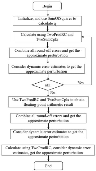
Figure 2. The flowchart of the compensated Goertzel algorithm with dynamic error estimates.

3.3. Computational Complexity

The $\mathtt{Horner}$ and its compensated algorithm $\mathtt{CompHorner}$ [12] are recalled in Algorithms 6 and 7. We shall use $\mathtt{TwoSum}$ and $\mathtt{TwoProd}$ instead of $\mathtt{TwoSumCplx}$ and $\mathtt{TwoProdCplx}$, while the inputs of Algorithm 7 are real floating-point numbers. A comparison of the computational costs of Algorithms 1 and 4–7 is shown in Table 2. As we can see, each of the compensated algorithms (i.e., $\mathtt{CompHorner}$ or $\mathtt{CompGoertzel}$) can be less expensive than the others in different cases. For example, $\mathtt{CompGoertzel}$ is half as expensive as $\mathtt{CompHorner}$ when $z\in \mathbb{C}$, $z\ne \pm 1$ and $a_n\in \mathbb{R}$. For $z\in \mathbb{C}$, $\left|z\right|\ne 1$ and $z\ne \pm 1$, the cost of $\mathtt{CompGoertzel}$ is also less than that of $\mathtt{CompHorner}$. Even in these cases, $\mathtt{CompGoertzelwErr}$ costs less than $\mathtt{CompHorner}$. However, for $z\in \mathbb{R}$, $\mathtt{CompGoertzel}$ is twice as expensive as $\mathtt{CompHorner}$ regardless of $a_n$.

Algorithm 5 Polynomial evaluation by compensated Goertzel algorithm with a dynamic error estimate

Function:  $[\overline{\omega }\left(z\right),\mu ]=\mathtt{CompGoertzelwErr}({\left(a_n\right)}_{n=0}^N,z)$ Require: $z=x+iy\in \mathbb{F}+i\mathbb{F}$, ${\left(a_n\right)}_{n=0}^N\in \mathbb{F}+i\mathbb{F}$ Ensure: $\overline{\omega }\left(z\right)\approx {\sum }_{n=0}^N{a}_n{z}^n$, $|\omega \left(z\right)-\overline{\omega }\left(z\right)|\le \mu$    $p=2x$    $[\widehat{q},\widehat{ϵq}]=\mathtt{SumOfSquares}(x,y)$    ${\widehat{b}}_N=a_N,{\widehat{b}}_{N+1}={\widehat{ϵb}}_N={\widehat{ϵb}}_{N+1}={\widehat{Eb}}_N={\widehat{Eb}}_{N+1}=0$    for  $n=N-1,N-2,...,1$       $[r_n,{\pi }_n]=\mathtt{TwoProdRC}(p,{\widehat{b}}_{n+1})$       $[s_n,{\sigma }_n]=\mathtt{TwoProdRC}(-\widehat{q},{\widehat{b}}_{n+2})$       $[t_n,{\eta }_n]=\mathtt{TwoSumCplx}(r_n,s_n)$       $[{\widehat{b}}_n,{\xi }_n]=\mathtt{TwoSumCplx}(t_n,a_n)$       ${\widehat{\ell }}_n={\pi }_n\oplus {\sigma }_n\oplus {\eta }_n\oplus {\xi }_n\ominus \widehat{ϵq}\otimes {\widehat{b}}_{n+2}$       ${\widehat{ϵb}}_n={\widehat{\ell }}_n\oplus p\otimes {\widehat{ϵb}}_{n+1}\ominus \widehat{q}\otimes {\widehat{ϵb}}_{n+2}$       ${\widehat{Eb}}_n=|{\widehat{\ell }}_n|\oplus \left|p\right|\otimes {\widehat{Eb}}_{n+1}\oplus \left|\widehat{q}\right|\otimes {\widehat{Eb}}_{n+2}$    end    $[r_0,{\pi }_0]=\mathtt{TwoProdRC}(x,{\widehat{b}}_1)$    $[s_0,{\sigma }_0]=\mathtt{TwoProdRC}(-\widehat{q},{\widehat{b}}_2)$    $[t_0,{\eta }_0]=\mathtt{TwoSumCplx}(r_0,s_0)$    $[{\widehat{b}}_0,{\xi }_0]=\mathtt{TwoSumCplx}(t_0,a_0)$    ${\widehat{\ell }}_0={\pi }_0\oplus {\sigma }_0\oplus {\eta }_0\oplus {\xi }_0\ominus \widehat{ϵq}\otimes {\widehat{b}}_2$    ${\widehat{ϵb}}_0={\widehat{\ell }}_0\oplus x\otimes {\widehat{ϵb}}_1\ominus \widehat{q}\otimes {\widehat{ϵb}}_2$    ${\widehat{Eb}}_0=|{\widehat{\ell }}_0|\oplus \left|x\right|\otimes {\widehat{Eb}}_1\oplus \left|\widehat{q}\right|\otimes {\widehat{Eb}}_2$    $\left[\varphi ,\psi \right]=\mathtt{TwoProdRC}(y,{\widehat{b}}_1)$    $\widehat{e}={\widehat{ϵb}}_0\oplus i({\widehat{ϵb}}_1\otimes y\oplus \psi )$    $\widehat{E}={\widehat{Eb}}_0\oplus i{\widehat{Eb}}_1\otimes y$    $\widehat{\omega }\left(z\right)={\widehat{b}}_0\oplus i\varphi$    $\overline{\omega }\left(z\right)=\widehat{\omega }\left(z\right)\oplus \widehat{e}$    $c=\widehat{\omega }\left(z\right)\oplus \widehat{e}\ominus \overline{\omega }\left(z\right)$    $\widehat{\alpha }=({\widehat{\gamma }}_{3N+1}\otimes \widehat{E})\oslash (1\ominus 6(N-1)\otimes u)$    $\mu =\left(\right|c|\oplus \widehat{\alpha })\oslash (1\ominus 2u)$

Table 2. Comparison of computational costs of $\mathtt{Horner},\mathtt{Goertzel},\mathtt{CompHorner},\mathtt{CompGoertzel}$ and $\mathtt{CompGoertzelwErr}$ algorithms.

Variates	Coefficients	$\mathbf{Horner}$	$\mathbf{Goertzel}$	$\mathbf{CompHorner}$	$\mathbf{CompGoertzel}$	$\mathbf{CompGoertzelwErr}$
$z\in \mathbb{R}$	$a_n\in \mathbb{R}$	2N	4N + 4	26N + 3	55N + 45	59N + 60
	$a_n\in \mathbb{C}$	4N	8N + 6	52N + 6	110N + 66	114N + 81
$z\in \mathbb{C}$ and $\left|z\right|\ne 1$	$a_n\in \mathbb{R}$	7N − 4	4N + 7	90N + 6	55N + 91	59N + 106
	$a_n\in \mathbb{C}$	8N	8N + 12	97N + 6	110N + 150	114N + 165
$z\in \mathbb{C}$, $\left|z\right|=1$ and $z\ne \pm 1$	$a_n\in \mathbb{R}$	7N − 4	3N + 4	90N + 6	34N + 26	39N + 41
	$a_n\in \mathbb{C}$	8N	6N + 9	97N + 6	68N + 90	72N + 105

Algorithm 6 Polynomial evaluation by the Horner algorithm

Function:  $\widehat{\omega }\left(z\right)=\mathtt{Horner}({\left(a_n\right)}_{n=0}^N,z)$ Require:   $z=x+iy\in \mathbb{F}+i\mathbb{F}$, ${\left(a_n\right)}_{n=0}^N\in \mathbb{F}+i\mathbb{F}$ Ensure:  $\widehat{\omega }\left(z\right)\approx {\sum }_{n=0}^N{a}_n{z}^n$    ${\widehat{b}}_{N+1}=0$    for  $n=N,N-1,...,0$       ${\widehat{b}}_n={\widehat{b}}_{n+1}\otimes z\oplus a_n$    end    $\widehat{\omega }\left(z\right)={\widehat{b}}_0$

Algorithm 7 Polynomial evaluation by the compensated Horner algorithm

Function:    $\overline{\omega }\left(z\right)=\mathtt{CompHorner}({\left(a_n\right)}_{n=0}^N,z)$ Require:   $z=x+iy\in \mathbb{F}+i\mathbb{F}$, ${\left(a_n\right)}_{n=0}^N\in \mathbb{F}+i\mathbb{F}$ Ensure:     $\overline{\omega }\left(z\right)\approx {\sum }_{n=0}^N{a}_n{z}^n$    ${\widehat{b}}_{N+1}={\widehat{ϵb}}_{N+1}=0$    for  $n=N-1,N-2...,0$       $[r_n,{\pi }_n]=\mathtt{TwoProdCplx}({\widehat{b}}_{n+1},z)$       $[{\widehat{b}}_n,{\sigma }_n]=\mathtt{TwoSumCplx}(r_n,a_n)$       ${\widehat{ϵb}}_n={\widehat{ϵb}}_{n+1}\otimes z\oplus {\pi }_n\oplus {\sigma }_n$    end    $\overline{\omega }\left(z\right)={\widehat{b}}_0+{\widehat{ϵb}}_0$

4. Numerical Experiments

In this section, we test the accuracy, performance and application of our algorithm. All numerical experiments are performed in IEEE-754 double precision as working precision.

4.1. Accuracy

The accuracy measurements in this part were found in MATLAB R2019b, and the exact results were obtained by the Symbolic Toolbox in order to compute the relative errors. As in [12], we considered the expanded form of the polynomial

$$\omega \left(z\right)={(z-1-i)}^n$$

(65)

at $z=1.333+1.333i$ for $n=3$:42, while the condition number varied from ${10}^3$ to ${10}^{33}$. The relative accuracy of the $\mathtt{Horner}$, $\mathtt{Goertzel}$, $\mathtt{CompHorner}$ and $\mathtt{CompGoertzel}$ algorithms as well as the theoretical bounds of $\mathtt{CompGoertzel}$ in Theorems 2 and 3 are exhibited in Figure 3. We can observe that the $\mathtt{CompGoertzel}$ algorithm, which had almost the same accuracy as the $\mathtt{CompHorner}$ algorithm, was absolutely stable when the condition number was smaller than ${10}^{16}$. Moreover, the numerical results and the error bounds had a good agreement, especially the running error bound, which was almost the same as the real relative errors, along with the results while the condition number was smaller than ${10}^{13}$.

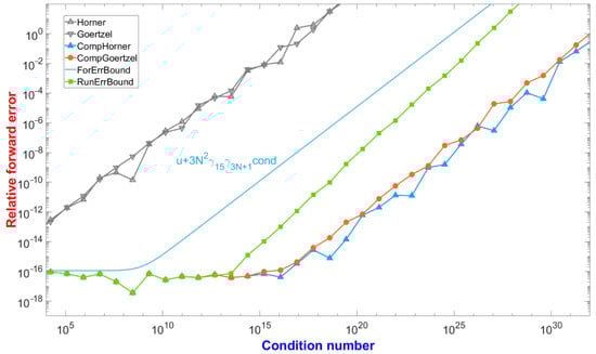
Figure 3. Accuracy of evaluation of $\omega \left(z\right)={(z-1-i)}^n$ at $z=1.333+1.333i$ for $n=3$:42.

4.2. Running Time

In this part, we show the practical performance of the $\mathtt{Goertzel}$, $\mathtt{CompGoertzel}$, $\mathtt{CompHorner}$ and $\mathtt{CompGoertzelwErr}$ algorithms in terms of measured computing time. The tests were performed in the following environments:

• Env1: Laptop with Intel Core i7-7700 CPU, 4 cores each at 3.6 GHz and with Microsoft Visual C++ 2012 with the default compiler option /od on Windows 7;
• Env2: Node of workstation with Intel Xeon E5-2697A CPU, 16 cores each at 2.6 GHz and with gcc 7.4.0 with the default compiler option-O0 on x86_64-Ubuntu-linux 18.04.

We generated the test polynomials with random coefficients in the interval $[-1,1]$, whose degree varied from 50 to 10,000 by a step of 50. The average time ratios for $\mathtt{CompGoertzel}$$/\mathtt{Goertzel}$, $\mathtt{CompGoertzel}/\mathtt{CompHorner}$, $\mathtt{CompGoertzelwErr}/\mathtt{CompGoertzel}$ and $\mathtt{CompGo}$$\mathtt{ertzelwErr}/\mathtt{CompHorner}$ are reported in Table 3 and Table 4, while the coefficients of the test polynomials were $a_n\in \mathbb{R}$ and $a_n\in \mathbb{C}$, respectively. As we can see, $\mathtt{CompGoertzel}$ was faster than $\mathtt{Goertzel}$ in practice, especially when testing in Linux. We note the good agreement of the numerical and theoretical results except for $\mathtt{CompGoertzelwErr}/\mathtt{CompHorner}$ while $z\in \mathbb{C}$, $\left|z\right|\ne 1$, $z\ne \pm 1$ and $a_n\in \mathbb{C}$ in Env2. This is because $\mathtt{CompHorner}$ takes more benefit than $\mathtt{CompGoertzelwErr}$ from the Fused-Multiply-and-Add instruction [34,35] and the instruction-level parallelism [7,8]. However, $\mathtt{CompGoertzelwErr}$ was still faster than $\mathtt{CompHorner}$ in this case in Env1.

Table 3. Theoretical computational complexity and measured running time ratios in $a_n\in \mathbb{R}$.

Variates		$\frac{\mathbf{CompGoertzel}}{\mathbf{Goertzel}}$	$\frac{\mathbf{CompGoertzel}}{\mathbf{CompHorner}}$	$\frac{\mathbf{CompGoertzelwErr}}{\mathbf{CompGoertzel}}$	$\frac{\mathbf{CompGoertzelwErr}}{\mathbf{CompHorner}}$
	Theoretical	13.75	2.12	1.07	2.27
$z\in \mathbb{R}$	Evn1	9.15	1.42	1.13	1.59
	Evn2	2.76	1.35	1.11	1.49
	Theoretical	13.75	61.14%	1.07	65.59%
$z\in \mathbb{C}$ and $\left|z\right|\ne 1$	Evn1	9.29	64.19%	1.13	72.22%
	Evn2	2.81	67.71%	1.1	74.14%
	Theoretical	11.33	37.79%	1.15	43.35%
$z\in \mathbb{C}$, $\left|z\right|=1$ and $z\ne \pm 1$	Evn1	6.53	44.09%	1.1	48.43%
	Evn2	2.22	53.66%	1.09	58.38%

Table 4. Theoretical computational complexity and measured running time ratios in $a_n\in \mathbb{C}$.

Variates		$\frac{\mathbf{CompGoertzel}}{\mathbf{Goertzel}}$	$\frac{\mathbf{CompGoertzel}}{\mathbf{CompHorner}}$	$\frac{\mathbf{CompGoertzelwErr}}{\mathbf{CompGoertzel}}$	$\frac{\mathbf{CompGoertzelwErr}}{\mathbf{CompHorner}}$
	Theoretical	13.75	2.12	1.04	2.19
$z\in \mathbb{R}$	Evn1	10.32	1.24	1.17	1.46
	Evn2	4.8	1.16	1.35	1.57
	Theoretical	13.75	1.13	1.04	1.18
$z\in \mathbb{C}$ and $\left|z\right|\ne 1$	Evn1	10.37	1.25	1.19	1.48
	Evn2	4.8	1.17	1.35	1.58
	Theoretical	11.33	70.13%	1.06	74.26%
$z\in \mathbb{C}$, $\left|z\right|=1$ and $z\ne \pm 1$	Evn1	7.21	84.61%	1.17	98.54%
	Evn2	3.67	89.22%	1.33	1.18

4.3. Application

The test environment in this part was the same as the accuracy measurements. We considered the polynomial in Equation (1) with $a_0,a_1,\dots ,a_N\in \mathbb{R}$ and $z_k=e^{-2\pi ki/(N+1)}$. Then, the DFT, which could be computed by the function “fft” with the polynomial’s coefficients in MATLAB returned $\omega \left(z_k\right)$ for $k=0,1,\dots ,N$. The $\mathtt{Goertzel}$ algorithm can also compute the DFT with the polynomial’s coefficients of specific indices $z_k$ in a vector. Figure 4 shows the relative errors of $\mathtt{Goertzel}$, $\mathtt{CompGoertzel}$, and $\mathtt{fft}$ applied to polynomials whose degrees varied from 50 to 1000 by a step of 10 with random coefficients in the interval $[-1,1]$, where the relative error was defined as $\parallel {\mathrm{res}}_{\mathrm{comput}}-{\mathrm{res}}_{\mathrm{exact}}{\parallel }_2/{\parallel {\mathrm{res}}_{\mathrm{exact}}\parallel }_2$. In Figure 4, although $\mathtt{fft}$ was more accurate than $\mathtt{Goertzel}$, the relative errors of $\mathtt{Goertzel}$ and $\mathtt{fft}$ were all increasing, while the degree of the polynomial grew. However, $\mathtt{CompGoertzel}$ always obtained full-precision accurate results in this test, and the relative error of our algorithm was ${10}^{15}$ to ${10}^{17}$, while the $\mathtt{fft}$ was from ${10}^{12}$ to ${10}^{15}$.

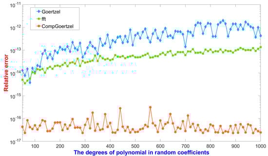
Figure 4. The relative errors of DFT for polynomials with random coefficients.

5. Conclusions

In this paper, we presented a compensated Goertzel algorithm with dynamic error estimation to evaluate polynomials in complex floating-point arithmetic. The forward error analysis and numerical experiments show that the algorithm can yield full working precision accuracy. Furthermore, although the algorithm is as precise as the compensated Horner algorithm, it is quicker in certain situations. The algorithm also performed well in the application of computing the DFT of specific indices.

References

- Peña, J.M.; Sauer, T. On the multivariate Horner scheme. Siam J. Numer. Anal. 2000, 37, 1186–1197. [Google Scholar] [CrossRef]
- Gentleman, W.M. An error analysis of Goertzel’s (Watt’s) method for computing Fourier coefficients. Comput. J. 1969, 12, 160–165. [Google Scholar] [CrossRef]
- Newbery, A.C.R. Error analysis for Fourier series evaluation. Math. Comput. 1973, 27, 639–644. [Google Scholar] [CrossRef]
- Wilkinson, J.H. Rounding Errors in Algebraic Processes; Courier Corporation: Englewood Cliffs, NJ, USA, 1994. [Google Scholar]
- Smoktunowicz, A.; Wróbel, I. On improving the accuracy of Horner’s and Goertzel’s algorithms. Numer. Algorithms 2005, 38, 243–258. [Google Scholar] [CrossRef]
- Bailey, D.H. Library for Double-Double and Quad-Double Arithmetric. Available online: http://www.nersc.gov/dhbailey/mpdist/mpdist.html (accessed on 18 February 2021).
- Louvet, N. Compensated Algorithms in Floating-Point Arithmetic: Accuracy, Validation, Performances; Université de Perpignan Via Domitia: Perpignan, France, 2007. [Google Scholar]
- Langlois, P.; Louvet, N. More Instruction Level Parallelism Explains the Actual Efficiency of Compensated Algorithm; Technical Report hal-00165020; DALI Research Team, University of Perpignan: Perpignan, France, 2007. [Google Scholar]
- Ogita, T.; Rump, S.M.; Oishi, S. Accurate sum and dot product. Siam J. Sci. Comput. 2005, 26, 1955–1988. [Google Scholar] [CrossRef]
- Graillat, S.; Langlois, P.; Louvet, N. Algorithms for accurate, validated and fast polynomial evaluation. Jpn. J. Ind. Appl. Math. 2009, 26, 191–214. [Google Scholar] [CrossRef]
- Graillat, S.; Morain, V. Error-free transformations in real and complex floating-point arithmetic. In Proceedings of the International Symposium on Nonlinear Theory and Its Applications, Vancouver, BC, Canada, 16–19 September 2007; pp. 341–344. [Google Scholar]
- Graillat, S.; Morain, V. Accurate summation, dot product and polynomial evaluation in complex floating-point arithmetic. Inf. Comput. 2012, 216, 57–71. [Google Scholar] [CrossRef]
- Graillat, S. An accurate algorithm for evaluating rational functions. Appl. Math. Comput. 2018, 337, 494–503. [Google Scholar] [CrossRef]
- Cameron, T.; Graillat, S. On a Compensated Ehrlich-Aberth Method for the Accurate Computation of All Polynomial Roots. Available online: https://hal.archives-ouvertes.fr/hal-03335604 (accessed on 16 March 2021).
- Jiang, H.; Barrio, R.; Li, H.; Liao, X.; Cheng, L.; Su, F. Accurate evaluation of a polynomial in Chebyshev form. Appl. Math. Comput. 2011, 217, 9702–9716. [Google Scholar] [CrossRef]
- Jiang, H.; Li, S.; Cheng, L.; Su, F. Accurate evaluation of a polynomial and its derivative in Bernstein form. Comput. Math. Appl. 2010, 60, 744–755. [Google Scholar] [CrossRef][Green Version]
- Delgado, J.; Peña, J.M. Algorithm 960: POLYNOMIAL: An Object-Oriented Matlab Library of Fast and Efficient Algorithms for Polynomials. ACM Trans. Math. Softw. 2016, 42, 1–19. [Google Scholar] [CrossRef]
- Kazal, N.Y.; Mukhlash, I.; Sanjoyo, B.A.; Hidayat, N.; Ozaki, K. Extended use of error-free transformation for real matrix multiplication to complex matrix multiplication. Siam J. Phys. Conf. Ser. 2021, 1821, 012022. [Google Scholar] [CrossRef]
- Ozaki, K. Error-free transformation of matrix multiplication for multi-precision computations. In Proceedings of the 19th International Symposium on Scientific Computing, Computer Arithmetic, and Verified Numerical Computations, Szeged, Hungary, 13–15 September 2021; Volume 33. [Google Scholar]
- Ozaki, K. An Error-Free Transformation for Matrix Multiplication with Reproducible Algorithms and Divide and Conquer Methods. J. Phys. Conf. Ser. 2020, 1490, 012062. [Google Scholar] [CrossRef]
- Ozaki, K.; Ogita, T. The Essentials of verified numerical computations, rounding error analyses, interval arithmetic, and error-free transformations. Nonlinear Theory Its Appl. 2020, 11, 279–302. [Google Scholar] [CrossRef]
- Blanchard, P.; Higham, D.J.; Higham, N.J. Accurately computing the log-sum-exp and softmax functions. IMA J. Numer. Anal. 2021, 41, 2311–2330. [Google Scholar] [CrossRef]
- Delgado, J.; Peña, J.M. Running relative error for the evaluation of polynomials. SIAM J. Sci. Comput. 2009, 31, 3905–3921. [Google Scholar] [CrossRef]
- Jiang, H.; Graillat, S.; Barrio, R.; Yang, C. Accurate, validated and fast evaluation of elementary symmetric functions and its application. Appl. Math. Comput. 2016, 273, 1160–1178. [Google Scholar] [CrossRef]
- Barrio, R.; Du, P.; Jiang, H.; Serrano, S. ORTHOPOLY: A library for accurate evaluation of series of classical orthogonal polynomials and their derivatives. Comput. Phys. Commun. 2018, 231, 146–162. [Google Scholar] [CrossRef]
- Croci, M.; Fasi, M.; Higham, N.J.; Mary, T.; Mikaitis, M. Stochastic rounding: Implementation, error analysis and applications. R. Soc. Open Sci. 2022, 9, 211631. [Google Scholar] [CrossRef]
- IEEE Standard 754-2008; Standard for Binary Floating Point Arithmetic. ANSI: New York, NY, USA, 2008.
- Clenshaw, C.W. A note on the summation of Chebyshev series. Math. Comput. 1955, 9, 118–120. [Google Scholar] [CrossRef]
- Szegö, G. Orthogonal Polynomials; American Mathematical Society: Providence, RI, USA, 1939. [Google Scholar]
- Knuth, D.E. The Art of Computer Programming: Seminumerical Algorithms, 3rd ed.; Addison-Wesley: Boston, MA, USA, 1998. [Google Scholar]
- Dekker, T.J. A floating-point technique for extending the available precision. Numer. Math. 1971, 18, 224–242. [Google Scholar] [CrossRef]
- Graillat, S.; Lauter, C.; Tang, P.T.; Yamanaka, N.; Oishi, S. Efficient Calculations of Faithfully Rounded I2-Norms of n-Vectors. ACM Trans. Math. Softw. 2015, 41, 1–20. [Google Scholar] [CrossRef]
- Higham, N.J. Accuracy and Stability of Numerical Algorithms, 2nd ed.; Society for Industrial and Applied Mathematics (SIAM): Philadelphia, PA, USA, 2002. [Google Scholar]
- Markstein, P. IA-64 and Elementary Functions: Speed and Precision; Prentice-Hall: Englewood Cliffs, NJ, USA, 2000. [Google Scholar]
- Nievergelt, Y. Scalar fused multiply-add instructions produce floating-point matrix arithmetic provably accurate to the penultimate digit. ACM Trans. Math. Softw. 2003, 29, 27–48. [Google Scholar] [CrossRef]
Publisher’s Note: MDPI stays neutral with regard to jurisdictional claims in published maps and institutional affiliations. |
© 2022 by the authors. Licensee MDPI, Basel, Switzerland. This article is an open access article distributed under the terms and conditions of the Creative Commons Attribution (CC BY) license (https://creativecommons.org/licenses/by/4.0/).