Design of an NSMCR Based Controller for All-Electric Aircraft Anti-Skid Braking System

Abstract

In this paper, a relative threshold event-triggered based novel complementary sliding mode control (NSMCR) algorithm of all-electric aircraft (AEA) anti-skid braking system (ABS) is proposed to guarantee the braking stability and tracking precision of reference wheel slip control. First, a model of the braking system is established in strict-feedback form. Then a virtual controller with a nonlinear control algorithm is proposed to address the problem of constraint control regarding wheel slip rate with asymptotical stability. Next, a novel approaching law-based complementary sliding mode controller is developed to keep track of braking pressure. Moreover, the robust adaptive law is designed to estimate the uncertainties of the braking systems online to alleviate the chattering problem of the braking pressure controller. Additionally, to reduce the network communication and actuator wear of AEA-ABS, a relative threshold event trigger mechanism is proposed to transmit the output of NSMC in demand. The simulation results under various algorithms regarding three types of runway indicate that the proposed algorithms can improve the performance of braking control. In addition, the hardware-in-the-loop (HIL) experimental results prove that the proposed methods are practical for real-time applications.

1. Introduction

The latest trend in the aviation industry is electrification, where studies on aircraft AEA-ABS equipped with electric motors and power electronic devices represent a growing field in aviation braking research [1]. The ABS is a vital device of an aircraft landing system to protect wheels from skidding during landing or in rejected takeoff situations. The electrical ABS differs from a traditional hydraulic ABS in several fundamental ways. For example, the power source is electric power rather than hydraulic power, the actuator is an electromechanical actuator (EMA) instead of a hydraulic piston, the cables replace hydraulic pipelines, and the electromechanical actuator controller (EMAC) [2] substitutes the hydraulic servo. At the same time, the electrical braking system can improve control accuracy, execute component-level fault diagnosis, avert leakage of hydraulic oil and threat of fire, and shorten long-winded pipelines. Thus, some of the latest aircraft types, such as B787 and Global Hawk [3,4], have been equipped the electrical braking system. Thanks to the ability to regulate and monitor the electromagnetic braking torque, this braking technique introduces an opportunity to apply advanced control theory in aircraft brake control [5,6,7,8].

The AEA-ABS is a complex high-order nonlinear electromechanical system [9] that involves model uncertainties and parameter variations, which pose challenges for control algorithm design. In the last decades, many traditional and advanced control techniques have been widely studied.

From the view of selection in manipulated variables, such as wheel deceleration rate, wheel speed difference, and wheel slip rate, various control methods have been studied over the past decades [10]. Wheel deceleration-based control strategies are widely equipped in the aircraft braking industry [11]; Moreover, the variant of these control strategies can bring certain advantages. For example, mixed wheel slip rate and deceleration (MSD) combines deceleration rate and wheel slip rate [10,12,13], which mitigates sensor noise impacts and improves control efficiency. However, the wheel slip rate-based control algorithms are commonly studied in the academic literature because of their high braking performance [7,14,15,16,17].

According to the nonlinear single-peak curve relationship between the wheel slip rate and the friction coefficient, the aircraft braking characteristic is divided into the stable and the unstable regions [14,18]. Once the braking system is trapped in the hazardous area, the wheels are prone to enter a deep skid state or even be locked up, which leads to a dramatic decrease in the lateral stability and maneuverability of the aircraft [14]. Thus, for the constraint control of wheel slip rate, various constraint control algorithms have been studied, such as model predictive control (MPC) [12], reference governor [16], and backstepping control based on the barrier Lyapunov function (BLF) [6,15]. Among these methods, the MPC calls for substantial computational resources for real-time application; the reference governor may induce delays in the slip rate control loop. With the backstepping method, the BLF based method can be designed systematically and intuitively to restrict output. However, the traditional BLF-based methods do not consider model uncertainty and external disturbance [17], so the derived control law cannot ensure asymptotic stability.

There has been much work conducted to address the problem of higher-order nonlinear characteristics in an aircraft braking system, for example, the traditional open-loop brake pressure control algorithm [19], the pressure-bias-modulated (PBM) algorithm [9], artificial neural networks, fuzzy control [20,21], local linearization and feedback linearization techniques [5], iterative learning control [17], and sliding mode control (SMC) [6,7]. However, these traditional algorithms present some disadvantages. For example, the open-loop control cannot compensate unknown disturbance; the PBM skid seriously at low speed; the artificial neural networks (ANN) calls for too much experiment data. Meanwhile, among these algorithms, the fuzzy algorithm relays too much on prior knowledge; the local linearization techniques cannot handle large disturbances; and the feedback linearization techniques easily lead to actuator saturation. The SMC is an appropriate choice, but this algorithm brings an excessive output chattering problem.

In traditional hydraulic braking algorithms, the brake control unit (BCU) acts as a black box [11] installed in aircraft in a traditional hydraulic braking system. It receives the main wheel speed and pilot braking command as input and outputs current to the drive pressure servo valve to generate braking torque to halt the airplane. It is a single closed-loop control architecture [7,8,9,10,12,13] combining control and drive. Unlike the hydraulic braking system, an electrical braking system has a novel system architecture [2]. Many problems will emerge, such as real-time performance deterioration and complicated implementation in embedded devices if the control framework inherits that of the hydraulic braking system.

To tackle these issues, we have carried out several innovative studies.

• A constraint control algorithm of slip rate is proposed to address the problem of the safety of aircraft electrical braking systems;
• A novel approaching law-based complementary sliding mode controller (NSMC) is developed to control the braking pressure with less chattering;
• In the AEA-ABS architecture, a relative threshold event triggering mechanism is proposed to reduce the network communication and CPU computation times in the braking process.

The structure of the remainder of this article is organized as follows. A mathematical model of the braking system is developed in Section 2. In Section 3, an event trigger-based robust adaptive control law is proposed. This controller is composed of a BLF-based controller and an event trigger-based NSMC with proven asymptotic stability proof and Zeno phenomenon avoidance. Simulations and experiments based on a certain UAV are conducted to evaluate the proposed algorithms in Section 4. In Section 5, hardware in the loop experiment shows that the proposed algorithm is practical in actual applications. A summary of the results and conclusions is deduced in the last chapter.

2. Dynamics of the AEA Anti-Skid Braking System

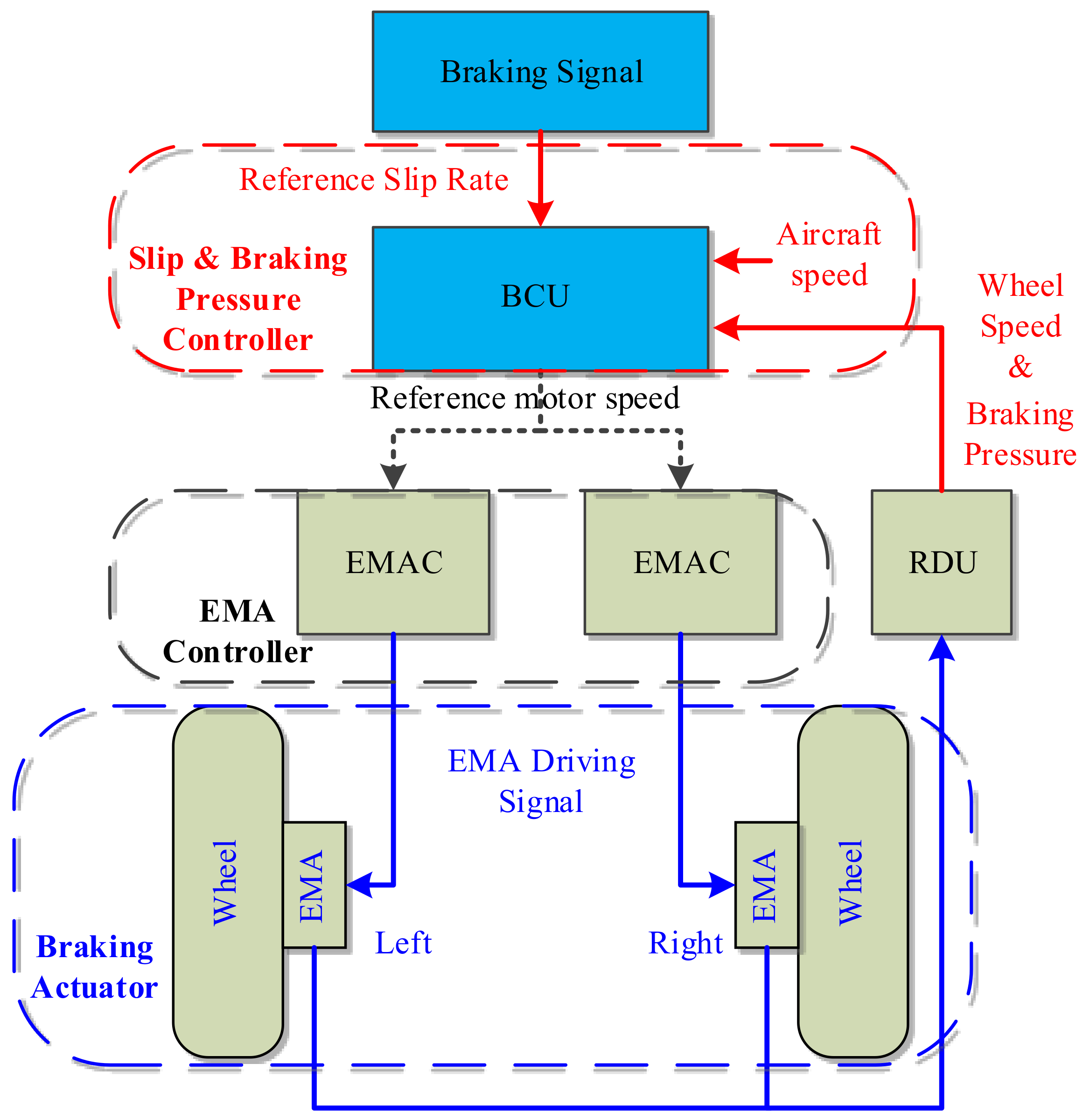
As shown in Figure 1, a typical aircraft AEA anti-skid braking system consists of the following subsystems [2]: BCU, EMA, EMAC, and wheel remote data acquisition unit (RDU). The principle is briefly described as follows. Once having received the braking commands from the pilot and sensor data from RDC, the BCU outputs control signals to EMACs through a communication bus after the anti-skid braking control (ABS) algorithm. Afterward, each EMAC tracks this signal to drive EMAs to generate braking torque to stop the aircraft. Here, EMAC acts as a well-studied speed servo [2,22,23], so we focused our efforts on control algorithms in BCU.

In Figure 1, the short dashed arrows represent network communication, and the rounded rectangles in red, black, and blue represent the ABS subsystem, EMA subsystem, and braking actuator, respectively. By retaining the essential characteristics of the aircraft braking system and making some assumptions [24], we construct the aircraft all-electric in the following braking system model.

2.1. Aircraft Fuselage Model

The results of the force analysis of the aircraft during ground roll are shown in Figure 2, whereby the longitudinal dynamic, vertical force balance, and pitch moment balance equations of the aircraft are listed as follows:

$$\left\{\begin{array}{c}m{\dot{V}}_x+F_x+n{F}_f+F_n-T_0=0\hfill \\ F_y+N_n+n{N}_m-mg=0\hfill \\ n{N}_{m}a+T_0{h}_t+n{F}_f{h}_c+F_n{h}_c-N_{n}b=0\hfill \end{array}\right.$$

(1)

where the following symbols represent different physical meanings: m for the aircraft mass; $V_x$ for the longitudinal speed of aircraft; $F_x$ for the aerodynamic drag; n for the number of main wheels; $F_f$ and $F_n$ for the between main wheels’ friction force and nose wheel friction force; $T_0$ for the residual thrust of the engine; $F_y$ for the lift; $N_m$ and $N_n$ for the nose and main wheel loads; g for the gravity acceleration; b and a for the distance from nose wheel and main wheel to the aircraft gravity center; $h_t$ for the length between engine thrust direction and aircraft gravity center; $h_c$ for the height of aircraft gravity center.

In Equation (1), the aircraft’s aerodynamic lift, aerodynamic drag, and residual engine thrust are calculated by the following equations.

$$\left\{\begin{array}{c}{F}_y=0.5C_y\rho S_y{V}_x^2\hfill \\ F_x=0.5C_x\rho S_x{V}_x^2\hfill \\ T_0=T_i+k_t{V}_x\hfill \end{array}\right.$$

(2)

where $C_x$ and $Cy$ are the drag and aerodynamic lift coefficients, respectively. $\rho$ represents the local air density, $S_x$ and $S_y$ are the aerodynamic drag area and lift area, respectively. $T_i$ is the initial residual thrust, and $K_t$ denotes the engine thrust coefficient.

By convention, the ground motion of aircraft is simplified as:

$$F_f{R}_g-B_w\dot{w}-T_b=J_w\dot{w}$$

(3)

where $R_g$, $B_w$, $J_w$, and w denote the radius, damping coefficient, moment of inertia, and wheel speed, respectively. $T_b$ signifies the braking torque:

$$T_b=K_b{P}_A$$

(4)

where $K_b$ indicates the torque conversion coefficient, a nonlinear function of the braking disc friction coefficient, the number of friction surfaces, and the diameters of discs.

2.2. Wheel-Runway Contact Dynamic

Due to the existence of braking torque, the wheel speed is always less than the longitudinal aircraft speed, whereby the slip rate $\lambda$ is defined as:

$$\lambda :=\frac{V_x-R_{g}w}{V_x}$$

(5)

It represents the ratio of the slip motion of the wheel concerning the runway. Obviously, $\lambda \in \left[0,1\right]$. For aircraft main wheel: $\lambda =0$ indicates a free rolling state, and $\lambda =1$ represents a totally locked-up state.

The aircraft slows down due to main wheel friction force $F_f$:

$$F_f=u{N}_m$$

(6)

which depends on the friction coefficient u and main wheel loads. Here we concentrate on the friction coefficient, which is affected by many factors, such as slip rate, aircraft speed, and runway conditions. From [6], there are many famous empirical models such as the Magic formula, the LuGre tire model, and the Rill model [25]. In this paper, we adopt the traditional Magic formula:

$$u=D·sin\left(C·arctan\left(B\lambda \right)\right)$$

(7)

where D, B, and C determine the model curve’s peak, shape, and stiffness, respectively. The typical parameter values for typical runway conditions are shown in

Table 1. Magic formula model parameters.

Runway Types	D	B	C	λd
Dry asphalt	1.28	23.99	0.52	0.12
Wet asphalt	0.85	33.82	0.34	0.10
Icy	0.05	306.39	0	0.05

, which are shown in Figure 3, where ${\lambda }_p$ is the slip rate constraint value and the intervals $\left[0,{\lambda }_p\right)$, and $\left[{\lambda }_p,1\right]$ are stable and unstable regions [5].

2.3. EMA Modeling

An EMA consists of a brushless DC motor, a reduction gear set, a ball screw, and force and electrical sensors. The EMA receives three-phase AC power from the EMAC to output mechanical power to generate braking force. This force is transformed into braking torque by amplifying the force in the gear set and the transition from the rotary motion to linear motion by the ball-screw set. During this process, the linear displacement of the screw in the actuator, namely, $x_{EMA}$, determines the output brake pressure with linear gain $c_b$:

$$P_A=c_b{x}_{EMA}$$

(8)

The equation of force on the ball screw is:

$${\dot{x}}_{EMA}=\frac{L_0{w}_m}{2\pi }$$

(9)

where $L_0$ is the lead of the ball screw and $w_m$ is the reference motor speed output to the EMAC.

2.4. System Overall Model

In the scope of the framework of the AEA anti-skid braking system, we choose the state variable in BCU as $X=\left[x_1;x_2\right]=\left[\lambda ;P_A\right]$ and the final control outputs as $u\left(t\right)=w_m$.

Taking derivatives of Equations (1), (2) and (5), we build the slip rate dynamic as:

$$\dot{\lambda }=\frac{w{R}_g{\dot{V}}_x-\dot{w}{R}_g{V}_x}{V_x^2}=\frac{1-\lambda }{m{J}_w{V}_x}\left\{J_w\left(T_0-F_x-un{N}_m-u_r{N}_n\right)+m{B}_{w}V-\frac{um{R}_g^2{N}_m}{1-\lambda }\right\}+\frac{K_b{R}_g}{J_w{V}_x}{P}_A$$

(10)

Combining Equations (8) and (9) yields the following brake pressure dynamic equation:

$${\dot{P}}_A=\frac{c_b{L}_0{w}_m}{2\pi }$$

(11)

Furthermore, taking the modeling uncertainties and external disturbances in Equations (10) and (11), we establish the all-electric system model as:

$$\left\{\begin{array}{c}{\dot{x}}_1=f_1\left(x_1\right)+\Delta f_1\left(x_1\right)+g_1\left(x_1,x_2\right)x_2+\Delta g_1\left(x_1,x_2\right)x_2+h\hfill \\ =f_1\left(x_1\right)+g_1\left(x_1,x_2\right)x_2+d_1\hfill \\ {\dot{x}}_2=g_2\left(x_1,x_2\right)w_m+\Delta g_2\left(x_1,x_2\right)w_m+q=g_2\left(x_1,x_2\right)w_m+d_2\hfill \\ y_1=x_1,y_2=x_2\hfill \end{array}\right.$$

(12)

where the nonlinear terms are shown as follows:

$$f_1\left(x_1\right)=\frac{1-\lambda }{m{J}_w{V}_x}\left\{J_w\left(T_0-F_x-un{N}_m-u_r{N}_n\right)+m{B}_{w}V-\frac{um{R}_g^2{N}_m}{1-\lambda }\right\}$$

$$g_1\left(x_1,x_2\right)=\frac{K_b{R}_g}{J_w{V}_x}$$

Moreover the control gain is:

$$g_2\left(x_1,x_2\right)=\frac{c_b{L}_0}{2\pi }$$

The unmodeled dynamics and external perturbations are merged into the lumped disturbances, namely, $d_1=\Delta f_1\left(x_1\right)+\Delta g_1\left(x_1,x_2\right)x_2+h$ and $d_2=\Delta g_2\left(x_1,x_2\right)w_m+q$, where $\Delta f_1$, $\Delta g_1$ and $\Delta g_2$ are the unmodeled dynamics, h and q are the external perturbations of the system.

2.5. Control Objectives

Given the system described by Equation (12), a controller is designed to satisfy the following goals:

• Design an anti-skid braking controller to prevent the wheels from falling into a deep skid and maintain the lateral stability of the aircraft;
• Design a braking pressure controller to track the virtual control in the backstepping controller and guarantee robustness to disturbance with less chattering;
• Design an event trigger mechanism for the network control structure of BCU and EMAC. The controller saves the amount of communication and computation under the premise of no Zeno phenomenon.

3. Control Strategy

According to the structure of the AEA anti-skid braking system and the proposed control objectives, the control structure shown in Figure 4 is designed in this paper. In Figure 4, $w_m$ and $i_m$ represent the motor stator current and speed in the EMA, respectively, ${\lambda }_d$ stands for the reference wheel slip rate, and the other symbols can be found in Equations (1), (5), and (12).

The whole system consists of three subsystems: BCU, the communication network, and EMAs. Therefore, the wheel slip rate controller, braking pressure controller, and network communication with event trigger mechanism are three parts to be designed in the following text.

3.1. Wheel Slip Rate Controller

When the slip rate falls into an unstable region, the friction coefficient decreases so dramatically that the wheels tend to be stuck in the deep slip state. This situation may lead to catastrophic outcomes for the aircraft. Therefore, a slip rate controller is imperative to maintain safety. From the properties of nonlinear and strong coupling in system Equation (12), the constraint control of wheel slip rate with stability guarantee is difficult to assure. To address this problem, we design a nonlinear wheel slip rate controller based on BLF.

Define the slip rate error as $e_1=x_{1d}-x_1$ and the error constraint variable as $k_b=x_{1p}-x_1$, where $x_{1p}$ is the slip rate stable boundary value. Define the symmetric logarithmic BLF as:

$$V_{BLF}=\frac{1}{2}ln\frac{k_b^2}{k_b^2-e_1^2}$$

(13)

The virtual control law for designing the optimal slip rate tracking is:

$$x_{2d}=\frac{1}{g_1}\left(-f_1+{\dot{x}}_{1d}-{\widehat{d}}_1+\frac{c_1{e}_1}{k_b^2-e_1^2}\right)$$

(14)

where the adaptive law of lumped disturbance is:

$${\dot{\widehat{d}}}_1={\mathrm{Proj}}_{{\widehat{d}}_1}\left\{-r_1{e}_1\frac{1}{k_b^2-e_1^2}\right\}$$

(15)

where $r_1$ is adaptive law gain, and the projection mapping is defined as:

$${\mathrm{Proj}}_{{\widehat{d}}_1}\left\{X\right\}=\left\{\begin{array}{c}0,if \left\{\begin{array}{c}{\widehat{d}}_1={\widehat{d}}_{1max} and X>0\hfill \\ {\widehat{d}}_1={\widehat{d}}_{1min} and X<0\hfill \end{array}\right.\hfill \\ X,otherwise\hfill \end{array}\right.$$

(16)

where ${\widehat{d}}_{1max}$ and ${\widehat{d}}_{1min}$ are the upper and lower bounds of the perturbation estimate, respectively. This mapping ensures the boundedness of the perturbation estimate.

3.2. Braking Pressure Controller

This section adopts a novel approaching law-based complementary sliding mode controller to track the braking pressure, where the robust adaptive law avoids lumped disturbance and the complementary sliding mode control alleviates the chattering phenomenon while preserving the control accuracy.

Compared with the traditional SMC, the complementary sliding mode controller (CSMC) introduces a generalized sliding mode surface and a complementary sliding mode surface to decrease the braking pressure tracking error rapidly. Here, we define the virtual control error $e_2=x_{2d}-x_2$, and the manifold of the CSMC:

$$\left\{\begin{array}{c}{S}_g=e_2+c{\int }_0^t{e}_{2}d\tau \hfill \\ S_c=e_2-c{\int }_0^t{e}_{2}d\tau \hfill \end{array}\right.$$

(17)

where $S_g$ and $S_c$ represent the generalized and complementary sliding mode surfaces, respectively. In addition, c is the sliding mode surface parameter. These two sliding mode surfaces satisfy:

$${\dot{S}}_c+c\left(S_g+S_c\right)={\dot{S}}_g$$

(18)

The SMC-based control output $u\left(t\right)$ consists of the equivalent control $u_{eq}$ and the switching control $u_{sw}$:

$$u\left(t\right)=u_{eq}+u_{sw}$$

(19)

where the equivalence control is:

$$u_{eq}=\frac{1}{g_2}\left({\dot{x}}_{2d}-{\widehat{d}}_2+c^2{\int }_0^t{e}_{2}d\tau -\frac{1}{2}{g}_1\frac{e_1}{k_b^2-e_1^2}\right)$$

(20)

where the adaptive law of lumped disturbance is represented as:

$${\dot{\widehat{d}}}_2={\mathrm{Proj}}_{{\widehat{d}}_2}\left\{-2r_2{e}_2\right\}$$

(21)

where $r_2$ is the adaptive law gain, and the projection mapping ${\mathrm{Proj}}_{{\widehat{d}}_2}\{\}$ is consistent with Equation (16).

The switching control is designed as follows based on the novel sliding mode approaching law:

$$u_{sw}=\frac{1}{g_2}\left(-{ϵ}_1{e}_2-{ϵ}_{2}sat\left(\frac{e_2}{\phi }\right)\right)$$

(22)

where ${\epsilon }_1$, ${\epsilon }_2$ are the controller design parameters and $sat(·)$ is a saturation function defined as follows:

$$sat\left(\frac{e_2}{\phi }\right)=\left\{\begin{array}{cc}1,& e_2\ge \phi \\ \frac{e_2}{\phi },& -\phi <e_2<\phi \\ -1,& e_2\le -\phi \end{array}\right.$$

(23)

where $\phi$ is boundary layer thickness.

3.3. Event-Triggered Mechanism Design

In previously proposed aircraft braking control architecture, a BCU and multiple EMACs and EMAs exist. The communications between BCU and EMACs rely on traditional avionics buses, such as ARINC429, RS-485, and MIL-STD-1553B; however, the communication bandwidth of these buses is relatively limited. We propose an event trigger mechanism to decrease the communication burden between BCU and EMACs without obvious control efficiency loss to address this problem. Compared to the fixed threshold trigger strategy, the relative threshold trigger strategy reduces the processor computing time in BCU.

Referring to the cascade control architecture, we consider the braking actuator containing EMACs, EMAs, and their sensors as a well designed servo unit. The details of the proposed event trigger architecture are shown in Figure 5. Here, the overall controller described by the red font is composed of BCU and ETM. The BCU consists of a slip rate and braking pressure controller, while the ETM is made up of an event trigger and a buffer. However, the communication network indicated in blue font and EMAs represented in black typeface fall out of the scope of this paper.

According to Figure 5, we design the event trigger control algorithm as follows:

$$\left\{\begin{array}{c}w\left(t\right)=u\left(t_j\right),\forall t\in \left[t_j,t_{j+1}\right)\hfill \\ t_{j+1}=inf\left\{t_{j+1}>t_j\left|\right|\delta \left(t\right)|\ge \xi \right\}\hfill \end{array}\right.$$

(24)

where $t_j$ denotes the time instant of the $j_{th}$ event trigger, $w\left(t\right)$ denotes the output of the controller under the $j_{th}$ trigger, the buffer acts as a cache for the latest successfully transmitted control signal $u\left(t_j\right)$, and $\delta \left(t\right)$ represents the difference between the current control and the last trigger control:

$$\delta \left(t\right)=u\left(t\right)-u\left(t_j\right)$$

(25)

and $\xi$ denotes the specific event triggering mechanism.

$$\xi =\left\{\begin{array}{c}C,fixed threshold event trig\hfill \\ \theta |u\left(t\right)|+\gamma ,relative threshold event trig\hfill \end{array}\right.$$

(26)

where C and $\theta$ and $\gamma$ are the design parameters of the fixed-threshold and relative-threshold event triggering mechanisms, respectively.

Then the relationship between $w\left(t\right)$ and $u\left(t\right)$ is shown as:

$$\left\{\begin{array}{c}w\left(t\right)=u\left(t\right)+\Lambda \left(t\right)\xi \hfill \\ \Lambda \left(t_k\right)=0,\Lambda \left(t_{k+1}\right)=1,|\Lambda \left(t\right)|\le 1\hfill \end{array}\right.$$

(27)

where $\lambda \left(t\right)$ is a tunable parameter. Thus, the actual output control transmitted to the communication network under the event-triggered mechanism becomes:

$$w\left(t\right)=\Lambda \left(t\right)\xi +\frac{1}{g_2}\left({\dot{x}}_{2d}-{\widehat{d}}_2+c^2{\int }_0^t{e}_{2}d\tau -\frac{1}{2}{g}_1\frac{e_1}{k_b^2-e_1^2}-{ϵ}_1{e}_2-{ϵ}_{2}sat\left(\frac{e_2}{\phi }\right)\right)$$

(28)

3.4. Stability Analysis

The previous sections design all the details of an aircraft anti-skid brake controller based on ETM. This section summarizes the main results to explain how to reach the control objectives described in Section 2.5.

At first, the following assumptions are made:

Assumption 1.

The given optimal slip rate is time continuous with continuous first- and second-order derivatives.

Assumption 2.

The map from the slip rate to the friction coefficient is a continuously differentiable function.

Assumption 3.

The aircraft’s longitudinal speed, wheel speed, and brake pressure can be obtained in real-time by sensors or other approaches.

Assumption 4.

The set-total disturbance in the system model is bounded and time-invariant.

According to the above assumptions and controller, the following theorems are obtained.

Theorem 1.

Noting the system plant depicted by Equation (12), the virtual controller in Equation (14) with adaptive law in Equation (15), and event-triggered mechanism-based control in Equation (28) with adaptive law in Equation (21) are adopted, then the system will be asymptotically stable.

Proof.

For the system model represented by Equation (12), we design a virtual controller based on the following Lyapunov function:

$$V_1=V_{BLF}+\frac{1}{2r_1}{\tilde{d}}_1^2=\frac{1}{2}ln\frac{k_b^2}{k_b^2-e_1^2}+\frac{1}{2r_1}{\tilde{d}}_1^2$$

(29)

where ${\tilde{d}}_1=d_1-{\widehat{d}}_1$ is the estimation error of the perturbation $d_1$, ${\widehat{d}}_1$ is the perturbation estimate, and $r_1$ is the perturbation estimate gain.

By taking the derivation of Equation (29), and substituting the definition of wheel slip rate error and Equation (12), we get the following equation:

$${\dot{V}}_1=\frac{e_1}{k_b^2-e_1^2}\left({\dot{x}}_{1d}-f_1-g_1{x}_2-d_1\right)+\frac{1}{r_1}{\tilde{d}}_1{\dot{\tilde{d}}}_1$$

(30)

From Equation (17), we get $x_2=x_{2d}-e_2$. With Assumption 4, the disturbance estimate error is described as ${\dot{\tilde{d}}}_1={\dot{d}}_1-{\dot{\widehat{d}}}_1=-{\dot{\widehat{d}}}_1$. Equation (30) is simplified as following:

$$\begin{array}{cc}\hfill {\dot{V}}_1& =\frac{e_1}{k_b^2-e_1^2}\left({\dot{x}}_{1d}-f_1-g_1{x}_{2d}+g_1{e}_2-d_1\right)+\frac{1}{r_1}{\tilde{d}}_1{\dot{\tilde{d}}}_1\hfill \\ \hfill & =\frac{e_1}{k_b^2-e_1^2}\left(-\frac{c_1{e}_1}{k_b^2-e_1^2}+g_1{e}_2-{\tilde{d}}_1\right)-\frac{1}{r_1}{\tilde{d}}_1\dot{\widehat{d}}\hfill \\ \hfill & =-c_1{\left(\frac{e_1}{k_b^2-e_1^2}\right)}^2+\frac{g_1{e}_1{e}_2}{k_b^2-e_1^2}-{\tilde{d}}_1\left(\frac{e_1}{k_b^2-e_1^2}-\frac{1}{r_1}{\dot{\widehat{d}}}_1\right)\hfill \end{array}$$

(31)

with the disturbance adaptive law in Equation (15) and the assumption that $e_2=0$, Equation (31) becomes:

$${\dot{V}}_1\le -c_1{\left(\frac{e_1}{k_b^2-e_1^2}\right)}^2\le 0$$

(32)

The Lyapunov function for the braking pressure controller is chosen as:

$$V_2=\frac{1}{2}\left(S_g^2+S_c^2\right)+\frac{1}{2r_2}{\tilde{d}}_2^2+V_1$$

(33)

where ${\tilde{d}}_2=d_2-{\widehat{d}}_2$ is the perturbation estimate. By combining Equations (19), (21) and (31) the derivation of $V_2$ can be derived as:

$$\begin{array}{cc}\hfill {\dot{V}}_2& =\left(S_g{\dot{S}}_g+S_c{\dot{S}}_c\right)+\frac{1}{r_2}{\tilde{d}}_2\left({\dot{d}}_2-{\dot{\widehat{d}}}_2\right)-\frac{g_1{e}_1{e}_2}{k_b^2-e_1^2}-V_{p1}\hfill \\ \hfill & =\left(S_g+S_c\right)\left({\dot{S}}_c+c{S}_g\right)-\frac{1}{r_2}{\tilde{d}}_2{\dot{\widehat{d}}}_2-\frac{g_1{e}_1{e}_2}{k_b^2-e_1^2}-V_{p1}\hfill \\ \hfill & =2e_2\left({\dot{e}}_2+c^2{\int }_0^t{e}_{2}d\tau +\frac{1}{2}\frac{g_1{e}_2}{k_b^2-e_1^2}\right)-\frac{1}{r_2}{\tilde{d}}_2{\dot{\widehat{d}}}_2-V_{p1}\hfill \\ \hfill & =2e_2\left({\dot{x}}_{2d}-g_2{w}_m-d_2+c^2{\int }_0^t{e}_{2}d\tau +\frac{1}{2}\frac{g_1{e}_2}{k_b^2-e_1^2}\right)-\frac{1}{r_2}{\tilde{d}}_2{\dot{\widehat{d}}}_2-V_{p1}\hfill \\ \hfill & =2e_2\left(-{ϵ}_1{e}_2-{ϵ}_{2}sat\left(\frac{e_2}{\phi }\right)\right)-{\tilde{d}}_2\left(2e_2+\frac{1}{r_2}Pro{j}_{{\widehat{d}}_2}\left\{-2r_2{e}_2\right\}\right)-V_{p1}\hfill \\ \hfill & =-2{ϵ}_1{e}_2^2-2{ϵ}_2{e}_{2}sat\left(\frac{e_2}{\phi }\right)-2{\tilde{d}}_2\left(e_2-Pro{j}_{{\widehat{d}}_2}\left\{e_2\right\}\right)-V_{p1}\hfill \end{array}$$

(34)

where $V_{p1}=-c_1{\left(\frac{e_1}{k_b^2-e_1^2}\right)}^2-{\tilde{d}}_1\left(\frac{e_1}{k_b^2-e_1^2}-\frac{1}{r_1}{\dot{\widehat{d}}}_1\right)\le 0$. This inequality ${\dot{V}}_2\le 0$ holds.

According to LaSalle’s invariance principle [22], the origin of the overall system is asymptotically stable. So, when $t\to \infty$, there exist $e_2\to 0$ and $e_1\to 0$, namely, $\lambda \to {\lambda }_d$. □

For event-triggered control, the following theorem guarantees the stability between two adjacent triggers.

Theorem 2.

Considering the closed-loop system consisting of an uncertain system in Equation (12), the nonlinear adaptive controller in Equation (28) with the event trigger the mechanism in Equations (24) and (26). There exists a lower bound of inter-execution intervals; namely, the following expression holds:

$$t_{lp}=inf\left\{t_{k+1}-t_k\right\}, \forall k\in {\mathrm{Z}}^{+}$$

(35)

Proof.

Taking the derivative of Equation (25) yields:

$$\frac{d\left|\delta \right|}{dt}=\frac{d}{dt}{\left(\delta \delta \right)}^{0.5}=\left(\delta \right)\dot{\delta }⩽\left|\dot{u}\left(t\right)\right|,\forall t\in \left[t_k,t_{k+1}\right)$$

(36)

As the derivative of $u\left(t\right)$ is a function of $x_1$, $V_x$, u, $x_{1d}$, and $e_1$, $e_2$, and due to the bounded characteristic of these signals, there exists a constant $\kappa$ > 0 such that $|\dot{u}\left(t\right)|⩽\kappa$. The lower bound $t_{lp}=\xi /\kappa$ on the execution interval between two adjacent events is obtained from $e\left(t_k\right)=0$ as well as ${lim}_{t\to t_{k+1}}e\left(t\right)=\xi$ so that the Zeno phenomenon [26] based on this event-triggered mechanism has been eliminated. □

4. Simulation Results and Analysis

To verify the validity of the algorithm proposed in this paper, a simulation model of the all-electric aircraft brake system is established in Simulink. Simulation scenarios in dry, wet, and icy runways are presented using traditional algorithms and the NSMCR algorithm proposed in this paper.

The aircraft speed and main wheel speed simulation results of different algorithms under dry, wet, and icy runway conditions are presented in Figure 6. From this figure, the aircraft can get a specific deceleration rate to halt the aircraft under all these algorithms. The braking time is about 22 s, 27 s, and 40 s for three different runways.

It is evident from Figure 7 that the NSMCR proposed in this paper exhibits the best transient performance in three runway conditions. The PID is prone to accelerate the braking mechanism wear with too much chattering, QLF contributes too much overshoot to exceed the safe slip rate region, and by contrast, BLF can constrain the slip rate to a safe interval. Furthermore, the SMC-based algorithms such as BSMC, NSMCF, and NSMCR combine the advantages of BLF and SMC to constrain the slip rate with better transient performance.

Figure 8 shows that the braking capacity in the three runways is almost halved in order, and the optimal friction coefficients are 0.8, 0.4, and 0.2. In every runway, BLF and NSMC (including NSMCF and NSMCR) have better asymptotic tracking performance with less oscillation than other traditional methods.

Figure 9 compares the output control chattering phenomenon under different control algorithms in three runway conditions. From part (a) of this figure, we conclude that PID significantly contributes to the control oscillation. As shown in part (b) of this figure, the SMC-based algorithms output stable control without much chattering after a short transition process. These stable control actions help reduce braking actuator wear to improve the reliability of the AEA anti-skid braking system.

The simulation results of lumped disturbances $d_1$ and $d_2$ are shown in Figure 10. The unmatched disturbance $d_1$ and matched disturbance $d_2$ tend to the actual value after a transition process. These estimated disturbances promote the control accuracy for their compensation of uncertainties, such as model uncertainties in the slip rate subsystem and braking pressure subsystem, disturbance in aircraft speed caused by aerodynamic interference, and wheel speed stemming from sensor noise.

Figure 11 shows the controller output frequency ratio of two ETM-based algorithms (NSMCF and NSMCR) and the traditional time-triggered algorithm (NSMC). Under the time-triggered algorithm, every output action is transmitted to the communication network. In event-triggered algorithms, these control actions are sent on demand. By averaging the whole sample in Figure 11, we conclude that communication and computation time is reduced to 63% (dry runway), 64% (wet runway), and 64% (ice runway) in NSMCF. In NSMCR, these data are 76% (dry runway), 75% (wet runway), and 75% (ice runway).

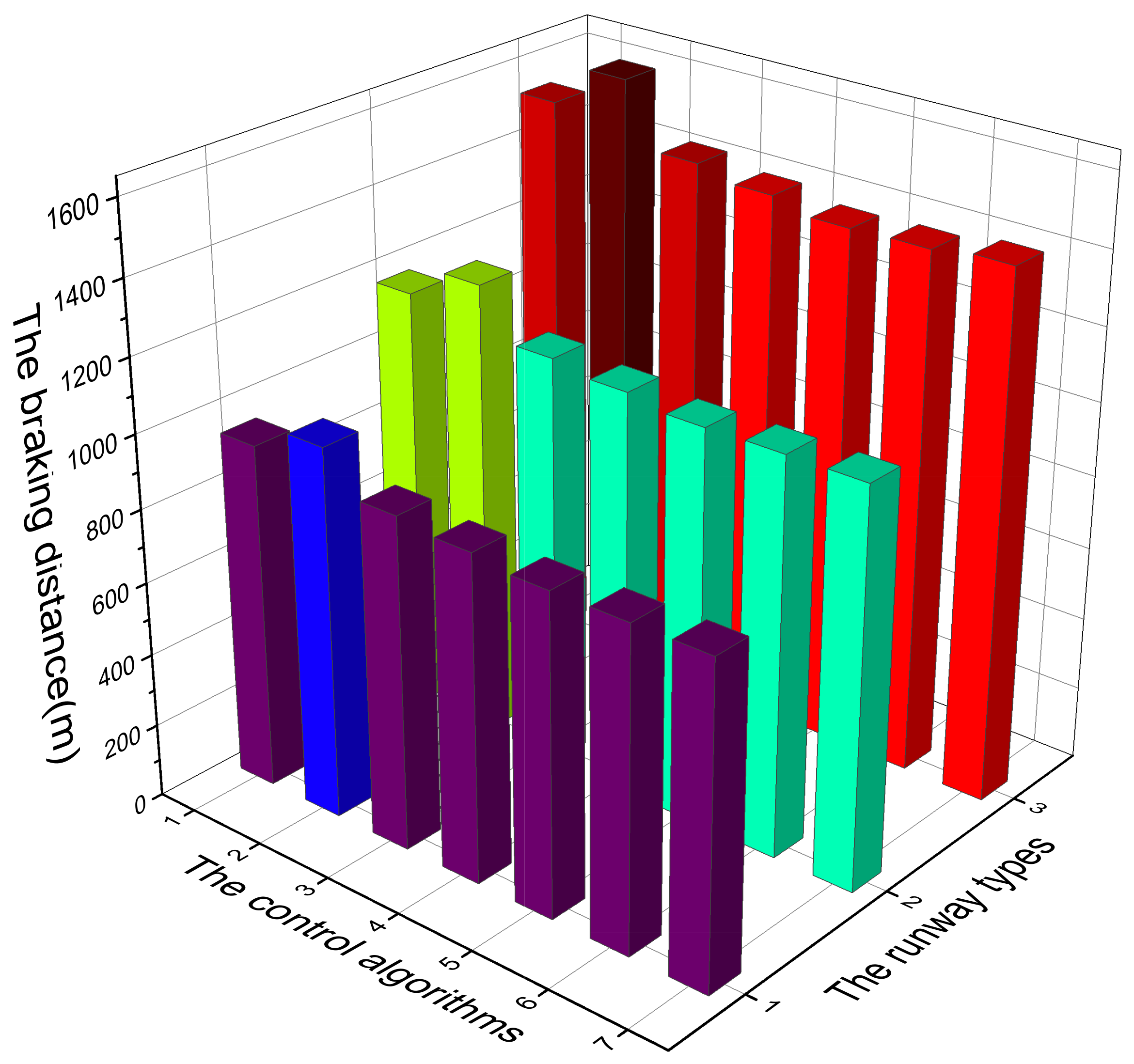
Finally, we studied the performance of the different algorithms under three runway scenarios. As shown in Figure 12 and Figure 13, these 3D bar figures represent the braking distance and average slip rate efficiency calculated as in [27], respectively. Note that the number in the control algorithm axis is described as follows: 1 = PID, 2 = QLF, 3 = BLF, 4 = BSMC, 5 = NSMC, 6 = NSMCF, and 7 = NSMCR. For the numbers in the runway type axis, 1 = dry runway, 2 = wet runway, and 3 = icy runway. From Figure 12, it can be seen that under the NSMCR algorithm, the braking distance is shorter than that of the traditional algorithms. Although adversely affected by ETM, the average slip rate efficiency of the NSMCF and NSMCR do not decrease much compared to NSMC. Taking Figure 11 and Figure 13, the NSMCR significantly reduces the control output transmission at the expense of a slight loss of efficiency.

5. Hardware in the Loop Experimental Results

The hardware in the loop setup consists of a real-time simulation computer, a simulation control client and an anti-skid brake controller, etc., and the experimental setup is shown in Figure 14. The controller is designed with TMS320F28335 and FPGA, which is suitable for engineering applications.

We built and debugged this DSP project in Code Composer Studio by combining peripheral drivers with this core control algorithm. Based on Linux-ihawk, the aircraft model runs in the SIMulation Workbench in real-time. The model exchanges data with external hardware through the PCI board and isolation module. With the assistance of these conditions, we obtain the following experimental results, as shown in Figure 15, Figure 16 and Figure 17.

Due to space constraints, we only present the experimental results of the PID and NSMCR algorithms under dry asphalt. In Figure 15 and Figure 16, the black, red, and blue solid lines represent the aircraft speed, wheel speed, and actual wheel slip rate, respectively. The friction coefficient, the braking pressure, and the motor speed are indicated with short black, red, and blue dashed curves. Comparing the two maps (Figure 15 and Figure 16) can conclude that the proposed NSMCR algorithm yields better performance than traditional algorithms. For example, faster convergence of the slip rate and friction coefficient is observed in the proposed controller.

At the same time, the controller output chattering phenomenon is avoided in the low-speed process. In Figure 16, the event trigger percentage of the relative threshold is shown as a short yellow dashed line. This plot shows that trigger rate drops to 20% in less than 0.2 s. Figure 17 shows the difference in the event trigger rate between the NSMCF and NSMCR algorithms. The difference is slight overall, but the relative trigger mechanism exhibits a lower trigger rate over time.

6. Conclusions

The present study lays the groundwork for future research for the network control of aircraft AEA anti-skid braking systems. It provides a hierarchical control architecture in an aircraft AEA anti-skid braking system with a novel control solution to this framework. This is a nonlinear adaptive backstepping CSMC algorithm based on the BLF and event triggering mechanism. This algorithm addresses two problems: the safe constraint control of slip rate and the limited communication bandwidth and BCU computation time.

Conclusions from this paper are presented as follows.

• The BLF-based nonlinear controller tackles the safe constraint of slip rate, preventing aircraft wheels from being skid or even locked up;
• The novel approaching law-based CSMC tracks the given braking pressure with less output chattering;
• The fixed and relative threshold-based event triggered mechanisms help reduce the communication data transmission and BCU computation time to improve the real-time performance in embedded practice in the proposed aircraft all-electric braking control architecture;
• The robust adaptive laws of these controllers compensate for the model uncertainty and external disturbance to further improve the stability.

Finally, all the algorithms and mechanisms are validated in MATLAB/Simulink simulation and hardware in the loop simulation. The study results show that our study has theoretical and practical value.