A Novel Stacking-Based Deterministic Ensemble Model for Infectious Disease Prediction

Abstract

Infectious Disease Prediction aims to anticipate the aspects of both seasonal epidemics and future pandemics. However, a single model will most likely not capture all the dataset’s patterns and qualities. Ensemble learning combines multiple models to obtain a single prediction that uses the qualities of each model. This study aims to develop a stacked ensemble model to accurately predict the future occurrences of infectious diseases viewed at some point in time as epidemics, namely, dengue, influenza, and tuberculosis. The main objective is to enhance the prediction performance of the proposed model by reducing prediction errors. Autoregressive integrated moving average, exponential smoothing, and neural network autoregression are applied to the disease dataset individually. The gradient boosting model combines the regress values of the above three statistical models to obtain an ensemble model. The results conclude that the forecasting precision of the proposed stacked ensemble model is better than that of the standard gradient boosting model. The ensemble model reduces the prediction errors, root-mean-square error, for the dengue, influenza, and tuberculosis dataset by approximately 30%, 24%, and 25%, respectively.

1. Introduction

Infectious diseases profess [1] a critical threat to the well-being of world populations. Epidemiological models have been used as practical [2] devices during flare-ups in human, animal, and plant populations. The capacity to precisely anticipate outbreaks provides a mechanism [3] for governments and healthcare sectors to react to the pandemics conveniently, empowering the impact to be lessened and limited assets to be spared. The early prediction of infectious diseases [4,5] is essential as it would considerably help mitigate the spread of the same and improve control capabilities. The proposed stacked ensemble model is used to accurately predict the future occurrences of infectious diseases viewed at some point in time as epidemics, namely, dengue, influenza, and tuberculosis.

Dengue fever (DF), induced by dengue viruses [6], is an intense mosquito-borne contamination. In 2018 and 2019, Hong Kong reported [7] 163 and 197 confirmed DF cases, including 29 and one local cases, and 134 and 196 imported [8] cases, respectively. Seasonal influenza [9,10], commonly known as the ‘flu’ prompted by influenza viruses, is a severe respiratory tract infection. In November 2019, a flare-up of H1N1 [7] was recorded in Iran, with 56 deaths and 4000 people hospitalized. Tuberculosis [11] is a significant communicable disease in Hong Kong. There are almost 4500 reported instances [7] of TB in Hong Kong, consistently every year.

Time series models [12] are of significant interest in the literature. These models analyze historical monitoring data to predict epidemiological behaviors. Bi et al. [13,14] employed an existing mathematical model to predict the Zika virus epidemic, suggesting that there is no practicality in using the continuous optimal control strategies, and they examined the epidemic control crisis of the infectious disease epidemic approach. Mahalle et al. [15] exploited predictive analytics to predict the spread of COVID-19 in the short term. Xi et al. [16] proposed a prediction model based on a deep residual network to predict influenza epidemics by integrating the spatio-temporal properties of influenza activity, allowing compelling influenza predictions at finer scales within urban areas. Zhang et al. [17] evaluated the performance of a dynamic Bayesian network (DBN) in infectious diseases surveillance. The study found that sample size is essential for identifying the dynamic relations among multiple variables. Siriyasatien et al. [18] addressed some challenges in epidemic outbreak prediction, such as developing robust dynamic forecasting models, handling big and uncertain data, and processing the semantics of exogenous data.

Predicting infectious diseases for decision-making is challenging. Moreover, a single model [19] may not be able to capture all the characteristics of the data structure accurately. However, ensemble learning can take care of this issue [20] by combining predictions from models with diverse qualities and leveraging each model’s strengths. Stacking is an ensemble learning technique, which combines heterogeneous learners to build a more robust model. Different models are stacked up; first, we have n number of base models that are trained parallelly, and the results of the base models are fed to train the Tier-2 model after which the predictions are obtained. This technique will help in exploiting the strengths of the models used to build the ensemble and hence enhancing the accuracy of the overall ensemble model. This study proposes a novel-stacking ensemble model in which the primary learning algorithms are auto-regressive integrated moving average (ARIMA), exponential smoothing (ETS), and neural network auto-regression (NNAR); these algorithms are selected based on their performance and predictive power. The secondary learning algorithm Gradient Boosting Regression Tree (GBRT) is used to combine the above three models. First, in the proposed ensemble, the individual models are optimally trained using the original disease training set, and then the fitted values of each model are combined using a weighted average technique. Based on the performance of each model, the weights are assigned manually. The combined weighted-fitted predictions are then fed to the XGBoost model. The parameters of the XGBoost model are tuned to train the model and to obtain robust forecast values. In light of the facts mentioned above and descriptions, the main contributions of this work are:

• Developing a weighted-stacked ensemble model using linear and nonlinear statistical models.
• Enhancing the prediction accuracy of the proposed model by optimally training each base model.
• Predicting the future occurrences of infectious diseases viewed at some point as epidemics, namely, dengue, influenza, and tuberculosis.

This study aims to enhance the prediction performance by lessening the prediction errors. The accuracy of the proposed stacked model is compared with the accuracy of the standard Gradient Boosting model. The accuracy measures used to check the performance are the root-mean-square error (RMSE) and mean absolute error (MAE). The study infers that the proposed model has a minor prediction error and performs better than the standard ensemble model. The remaining manuscript is organized as follows. Section 2 discusses the work related to some existing models developed in the past. Section 3 describes the data collection and preprocessing steps, and explains the implementation steps and the methods used to develop the proposed model. Results and Discussions are briefly summarized in Section 4 and Section 5. Section 6 concludes the manuscript and suggests further works in the topic.

2. Related Work

Zhang et al. [12] described a study to evaluate and compare four-time series models, namely the regression model, exponential smoothing model, autoregressive integrated moving average (ARIMA), and support vector machine (SVM). The data for nine types of infectious diseases were collected through mainland China’s national public health surveillance system. The results inferred that no single model is superior to others, and SVM outperformed ARIMA and the other two models for most cases of infectious disease. Mehrmolaei and Keyvanpour [21] reviewed significant work examining the time series forecasting models in statistical application areas. They proposed a novel approach using a mean estimation error for time series forecasting to enhance the ARIMA model. The results indicated that the procedure described can improve the accuracy in predicting time series data. Song et al. [22] predicted influenza incidences using the time series analysis method. Before proceeding to implement the various models, the dataset was checked for the presence of a time series component, i.e., seasonality. If there is a presence of seasonality, the seasonal autoregression integrated moving average (SARIMA) is used, and if the dataset shows no seasonality, then the ARIMA model is used.

Hyndman et al. [23] comprehended all the exponential smoothing models in a state-space framework, which allowed the computation of prediction intervals, likelihood, and model selection criteria. The proposed model by the authors supposedly performs better for short-term forecasts, i.e., six-periods-ahead forecast. Xuan et al. [24] proposed a novel prediction technique based on gradient boosting decision trees for predicting candidate drug–target interactions. The model ascertains multiple decision trees with the elicited features and, thus, assists in lessening the influence of class imbalance. The preliminary results show that the gradient boosting-based model outperforms other state-of-the-art approaches for drug–target interaction prediction.

Wang et al. [19] compared the performance of conventional time series models and deep learning algorithms in the case of malaria prediction and examined the application advantage of stacking strategies in the domain of infectious disease forecasting. The “ARIMA, STL + ARIMA, BP-ANN, and LSTM” network models were applied individually to malaria and meteorological data of Yunnan Province from 2011 to 2017. The predictive accuracy of each model was evaluated using: “root-mean-square error” (RMSE), “mean absolute scaled error” (MASE), and “mean absolute deviation” (MAD) measures. Moreover, “gradient-boosting regression trees” (GBRTs) were used to combine the above four models in the stacking framework. The RMSEs of the four base models were 13.176, 14.543, 9.571, and 7.208; the MASEs were 0.469, 0.472, 0.296, and 0.266; and the MAD were 6.403, 7.658, 5.871, and 5.691, respectively. The RMSE, MASE, and MAD values of the ensemble model decreased to 6.810, 0.224, and 4.625, respectively, after using the stacking framework.

3. Materials and Methods

Ensemble learning [25] consolidates predictions from different models to improve a model’s performance or reduce the probability of a poor selection. For example, in the gradient boosting ensemble technique [19], models are built by learning from past mistakes in every iteration. If some model has poor predictions, the other upcoming models try to compensate this by performing comparatively well on the dataset and improving the resulting ensemble’s performance. By combining individual models, the ensemble model tends to reduce the bias and the variance [26], the two most essential features expected from a model, to generate a robust learner that is more flexible and less data-sensitive.

The variant methods for combining diverse learners [27] are bagging, boosting, and stacking (Figure 1). Unlike bagging and boosting, stacking trains the tier-2 learner by combining the predictions from a bunch of different models as base/tier-1 learners trained in parallel. Stacking achieves the [27] independence between diverse learners by parallel-combining base models and the dependence between learners by introducing the meta-learner sequentially. Consequently, it leads to a higher forecast precision and a lower possibility of overfitting. A general stacking framework is shown in Figure 2. In the proposed model, tier-1 learners are ARIMA, ETS, and NNAR models, and the tier-2 learning algorithm is Extreme Gradient Boosting.

The data [28] for dengue fever, influenza, and tuberculosis infectious diseases with respect to time are shown in Figure 3. The three different health problems, dengue, influenza, and tuberculosis, are chosen to check the robustness of the developed ensemble model on various application domains.

3.1. Development of Stacked Ensemble Model

The implementation steps of the proposed model are shown in Figure 4. The steps involved in the process of developing the novel-Stacked Ensemble model are:

• Collect the monthly datasets for each dengue, influenza, and tuberculosis disease.
• Divide each dataset into a training set and a testing set. Each dataset comprises ten years of monthly reported cases, of which 80% of the data (from the year 2010 to 2017) are taken as the training set and 20% (the years 2018 and 2019) are taken as the testing set.
• The datasets are not skewed much and are ordinarily distributed; hence, no data transformation steps are required.
• Each training set is then passed as input to the ARIMA, ETS, and NNAR models in parallel, and the models are trained until they generate minimum training errors. As the datasets have seasonal dependencies, these are removed by differencing the datasets according to their seasonality, after which they are fed to the base models.
• The fitted values from each model are then combined using the weighted average technique. The weights are assigned manually based on the training accuracy of each model. The model with higher training accuracy is given a higher weight. This step is performed so that the model whose fitted and actual values do not differ much is given more weightage than others to improve the accuracy of the stacked model.
• The fitted values resulting from the above step are then fed to the gradient boosting algorithm. The algorithm’s parameters, the number of times the algorithm is executed (nround), and the learning rate of the model (eta) are manually tuned. Tuning of the algorithm increases the overall performance and hence generates fewer errors.
• The accuracy of the proposed model is then estimated by evaluating its performance metrics in terms of errors. After the model is trained, the proposed model is used to predict 2018 and 2019. The predicted and the test set values are then compared to calculate the errors.

All the coding, implementation, and development steps are executed using the R programming language and analyzed in RStudio software. Algorithm 1 is the pseudocode for developing the stacked ensemble model.

Algorithm 1 Generating Stacked Ensemble Model

Input: Disease Time Series Data D = {d1, d2, ……, dn}                               Total number of observations n = 120                               Sampling Frequency f = 12           Base Learners Predictions B = {B1, B2, ……, Br} where B = avg(B1(d), B2(d), ……, Br(d))                               Meta Learner Predictions M(B) Output: Ḿ (Prediction for unknown/test data) 1. Disease dataset is collected and sampled based on the frequency f. 2. Sampled dataset is divided into train and test sets: Train = n * 0.8 Test = n * 0.2 3. STL decomposition is done for training dataset: For i = 1 to Train do Td ← decompose(di) //Decompose the data into trend, seasonal and random components           //Stacked Ensemble Learning 4. Decomposed data is fed to Base Learners: For i = 1 to r do                   For j = 1 to Train do                                      Bi = B(dj) 5. Integrating the predictions from base learners: For i = 1 to r do WP ← Σ wi * Bi //Integrating predictions by weighted average technique // wi is the weight assigned to each base learner 6. Training of Meta-Learner: M ← M(WP) 7. Making predictions or forecasting for test data: For i = 1 to Test do                     Ḿ ← M(di)

3.1.1. Training of Auto-Regressive Integrated Moving Average Model

ARIMA models [29] are the most prevailing models for anticipating a time series that can be made stationary by differencing if necessary. The ARIMA model’s fundamental notion is to treat the time-series data as a random series and fit the time series data by applying a mathematical model. The disease time-series datasets collected are seasonal; therefore, the SARIMA model is adopted, represented as ARIMA (p,d,q) (P,D,Q)n, where ‘p’ is the number of lag observations—“order of autoregression,” ‘d’ is the degree of “differencing” to make data stationary, ‘q’ is the number of “lagged forecast errors”—“order of moving average,” (P,D,Q) are the seasonal parts similar to the nonseasonal parts of the model, and n is the “number of observations per year,” which is 12 for monthly disease datasets. The “autocorrelation” (ACF) and “partial autocorrelation” (PACF) plots can be used to calculate the p and q values of the model. The lag at which the ACF plot converges to zero is the value for the q parameter, and the point at which the PACF plot reaches zero is the value for the p parameter. The ARIMA model equation [29] when the data are seasonal is as follows:

$$\begin{gathered} {\widehat{O}}_t=\left({\delta }^d{\delta }_n^D{o}_t\right)=\left\{\raisebox{1ex}{$\theta \left(B\right)\mathit{\theta }\left(B^n\right){ϵ}_t$}\!\left/ \!\raisebox{-1ex}{$\phi \left(B\right)\mathit{\phi }\left(B^n\right)$}\right.\right\} \\ \mathrm{where}: \\ \phi \left(B\right)=1-{\phi }_{1}B-\dots -{\phi }_p{B}^p \\ \theta \left(B\right)=1+{\theta }_{1}B+\dots +{\theta }_q{B}^q \\ \mathit{\phi }\left(B^n\right)=1-{\mathit{\phi }}_1{B}^n-\dots -{\mathit{\phi }}_P{B}^{Pn} \\ \mathit{\theta }\left(B^n\right)=1+{\mathit{\theta }}_1{B}^n+\dots +{\mathit{\theta }}_Q{B}^{Qn} \end{gathered}$$

(1)

$o_t$ represents the actual dataset value at time $t$, ${\widehat{O}}_t$ represents the fitted value from ARIMA at time $t$, ${ϵ}_t$ is the random error/noise at time $t$, ${\delta }^d$ is nonseasonal differencing and ${\delta }_n^d$ is seasonal differencing, $\phi , \theta$ are used as nonseasonal autoregressive (AR) and moving average (MA) components, respectively, and $\mathbf{\phi }, \mathbf{\theta }$ are used for seasonal AR and MA components, respectively. $B$ is the backshift operator, which causes the observation that it multiplies to be shifted backward in time by one period. This operator simplifies the ARIMA equation, which is otherwise complicated because of the differencing term.

3.1.2. Training of Exponential Smoothing Model

The exponential Smoothing Method [30] is a family of forecasting models that uses weighted averages of past observations to forecast new values. The purpose is to give more attention to immediate values in the series. It combines Error (E), Trend (T), and Seasonal (S) components in smoothing estimation. Each term can be combined either in an additive (A) or multiplicative (M) manner or excluded (N) from the model. Generally, the model is represented as ETS (A/M, A/M/N, A/M/N). The forecast equation [30] for the ETS model, which fits the influenza dataset, is written as:

$$\begin{gathered} \mathrm{ETS}\left(\mathrm{A},\mathrm{N},\mathrm{A}\right)={\widehat{F}}_{t+h|t}=l_{t-1}+s_{t-n}+e_t \\ \mathrm{Level}: l_t=l_{t-1}+\alpha e_t \\ \mathrm{Seasonal}: s_t=s_{t-n}+\gamma e_t \\ \mathrm{where} 0\le \alpha \le 1;0\le \gamma \le 1-\alpha \end{gathered}$$

(2)

${\widehat{F}}_{t+h|t}$ represents forecast values, $f_t$ is the training data at time $t$, $h$ is the number of data points to be predicted, $e_t=f_t-{\widehat{F}}_{t|t-1}$ is the forecast error at time $t$, $l_t$ is the unknown level/state, $s_t$ is the unknown season/state, and $\alpha$ and $\gamma$ are the smoothing parameters.

3.1.3. Training of Neural Network AutoRegression Model

Artificial neural networks (ANN) [31] are prediction models used to mimic the basic mathematical patterns that the brain shows. “A neural network is a layered network of neurons, the predictors as inputs in the bottom layer, and the forecasts as outputs in the top layer” [19]. Sometimes a hidden/middle layer of “neurons” may be present. The NNAR model is where the lagged data points of the time series data are given as inputs to the neural network. The model is represented as NNAR (p,P,k), where p and P are the number of nonseasonal and seasonal immediate datapoints used as predictors, and k represents the number of hidden layer nodes. The equation [31] of the NNAR model for the given data at the time is written as:

$${\widehat{P}}_t=f\left(o_{t-1}\right)+{\epsilon }_t$$

(3)

${\widehat{P}}_t$ represents the forecast values, $f$ is the neural network function with $k$ hidden nodes, and ${ϵ}_t$ is normally distributed error series with a constant variance.

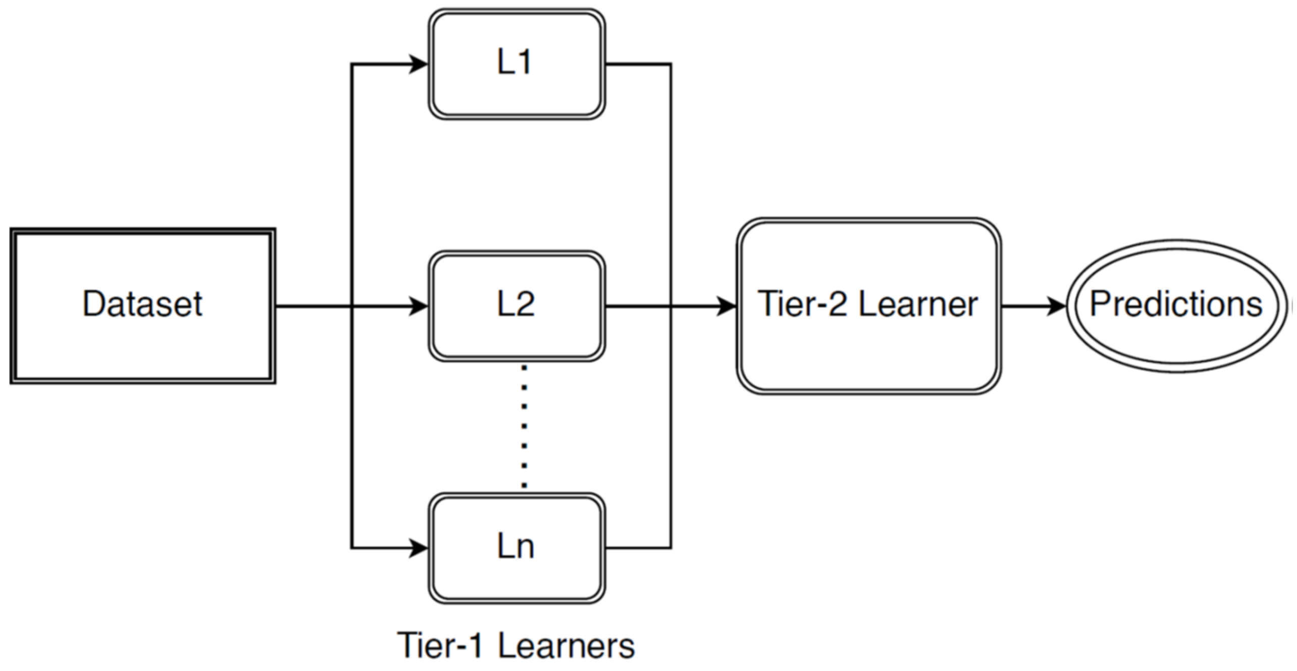
3.1.4. Construction of Tier-2 Learner Algorithm, GBRM

Gradient boosting is a machine learning [27,32] method for regression and classification problems, to design a prediction/ensemble [33] model that is a weighted sum of weak learners. The weak learners are aggregated to form robust learners iteratively. The models trained individually are combined before modeling the gradient boosting algorithm to forecast infectious diseases. Let ${\widehat{O}}_t$, ${\widehat{F}}_t$, and ${\widehat{P}}_t$ be the fitted values from the ARIMA, ETS, and NNAR models, respectively. Based on the training accuracy, which is the root-mean-square error of the model, which is shown in

Table 1. Training errors (RMSE) of Tier-1 models.

	Dengue	Influenza	Tuberculosis
ARIMA	11.42	13.55	36.23
ETS	9.75	12.23	31.23
NNAR	9.99	17.60	36.43

for each model, weights are assigned manually to these heterogeneous models. The fitted values from the models are multiplied by their corresponding weights and summed up. Monte Carlo simulations are applied to find the suitable weights corresponding to each model. The resulting weighted average values are given as:

$${\widehat{W}}_t=w_1\ast {\widehat{O}}_t+w_2\ast {\widehat{F}}_t+w_3\ast {\widehat{P}}_t$$

(4)

Immediately, these weighted average values are fed to the tier-2 models. The proposed model uses the XGBoost algorithm as a tier-2 learner algorithm, which implements gradient boosting regression/decision trees.

3.2. Performance Analysis

In this study, two error-index parameters are used to evaluate the overall performance of the proposed stacking ensemble model. The RMSE and MAE of different prediction models are compared to measure the prediction [8] accuracy. Assuming ${\widehat{m}}_t$ as the predicted value of the diseases at time $t$ and $o_t$ as the actual dataset value at time $t$, the equations [34] for the error metrics mentioned above are as follows:

$$\mathrm{RMSE}=\raisebox{1ex}{$\sqrt{{{\displaystyle \sum }}_{t=1}^T{\left(o_t-{\widehat{m}}_t\right)}^2}$}\!\left/ \!\raisebox{-1ex}{$T$}\right.$$

(5)

$$\mathrm{MAE}=\raisebox{1ex}{${{\displaystyle \sum }}_{t=1}^T\left|o_t-{\widehat{m}}_t\right|$}\!\left/ \!\raisebox{-1ex}{$T$}\right.$$

4. Result Analysis

4.1. Data Collection and Preprocessing

The data are collected from the “official government website of Hong Kong” [28] for all three diseases. In the modeling process, for each disease, the data from 2010 to 2017 are used as the training set with 96 observations, and the data for the year 2018 and 2019 are used for testing purposes with 24 observations. The data are also decomposed into trend and seasonal components to observe the pattern before modeling. The dengue dataset shows an “increasing trend.” The influenza dataset shows an increasing trend until 2018, and then the cases decrease in 2019. The tuberculosis dataset shows a “decreasing trend.” All the datasets have a periodical seasonality drive. The peak period for the influenza disease by observing the dataset is from January to March. February contributes 9.93% of the total cases, followed by March and January, which is 9.54% and 9.47% of the actual cases, respectively. This seasonal effect must be removed before modeling using the first-order or second-order differencing of the dataset depending upon the method used.

4.2. Results

The dengue fever, influenza, and tuberculosis datasets have 120 observations comprising ten years of data from 2010 to 2019. For training and validation purposes, these datasets are divided into train and test sets. Over the training set, the tier-1 models of the proposed method are applied one by one in parallel.

From the forecast package in R, auto.arima() is used to train the ARIMA model. The best model generated from the monthly dengue dataset is ARIMA (0,1,1)(1,0,0)12, differentiating the data once to make it stationary, having one nonseasonal MA term and one seasonal AR term. This model is chosen because it has the lowest second-order Akaike Information Criteria (AICc) of 573.99 compared to other model parameters. The model equation is written as:

$${\widehat{O}}_t={\delta }^1{o}_t=\raisebox{1ex}{$\left(1-0.90B\right)\ast {ϵ}_t$}\!\left/ \!\raisebox{-1ex}{$\left(1-0.25B^{12}\right)$}\right.$$

(6)

To train the ETS model for the dengue dataset, ets() is used from the forecast package in R. The ETS (A,N,A) model best fits the data with AICc of 401.31. The model contains an additive error, no trend, and seasonal additive components. The forecast equation of the model is shown below:

$$\begin{gathered} {\widehat{F}}_{t+h|t}=l_{t-1}+s_{t-n}+e_t \\ {l}_t=l_{t-1}+0.2097\ast e_t \\ {s}_t=s_{t-n}+0.0001\ast e_t \end{gathered}$$

(7)

From the nnfor package in R, nnetar() is used to train the NNAR model on the dengue dataset. After applying the model multiple times, the NNAR (11,1,6) model best fits the data. It indicates that 11 immediate values of the dataset are used as predictors, which is, by default, chosen by optimally fitting the linear model to the seasonally adjusted data. As the p-value is not specified while applying the model, it is, by default, 1 for seasonal time series, and six hidden nodes are there in the network, calculated as $\raisebox{1ex}{$p+P+1$}\!\left/ \!\raisebox{-1ex}{$2$}\right.$, i.e., $\raisebox{1ex}{$11+1+1$}\!\left/ \!\raisebox{-1ex}{$2$}\right.$. The model creates an average of 20 networks, each of which is a 12-6-1 network, which means twelve input/predictor nodes (11 nonseasonal and one seasonal), six hidden nodes, and one output node. The network is implemented iteratively for forecasting. The first network out of the 20 networks is implemented. The fitted values of this network are used as inputs for the second network. This process continues until all the requisite forecasts are calculated.

Similarly, ARIMA (0,0,1)(1,0,0) 12 best fits the influenza dataset, indicating one non-seasonal MA term and one seasonal AR term. The data are stationary; therefore, no differencing is required. The model has the lowest AICc of 644.44. The model equation can be written as:

$${\widehat{O}}_t=\raisebox{1ex}{$\left(1+0.57B\right)\ast {ϵ}_t$}\!\left/ \!\raisebox{-1ex}{$\left(1-0.29B^{12}\right)$}\right.$$

(8)

The ETS (A,N,A) best fits the data with the lowest AICc value of 434.53, indicating an additive error, no trend, and seasonal additive components. The forecast equation can be written as:

$$\begin{gathered} {\widehat{F}}_{t+h|t}=l_{t-1}+s_{t-n}+e_t \\ {l}_t=l_{t-1}+0.198\ast e_t \\ {s}_t=s_{t-n}+0.00011\ast e_t \end{gathered}$$

(9)

The NNAR (7,1,4) best fits the data after applying it multiple times, indicating seven nonseasonal predictors, one seasonal predictor, and four hidden nodes, all calculated the same as before. The model creates an average of 20 networks, each of which is an 8-4-1 network indicating eight input/predictors’ nodes—seven nonseasonal and one seasonal— four hidden nodes, and one output node.

ARIMA (0,0,0)(1,1,0)12 best fits the tuberculosis dataset, indicating only one seasonal AR term. Seasonal differentiation is required to make the series stationary. This model is chosen because it has the lowest AICc of 473.13 compared to other model parameters. The model equation can be written as:

$${\widehat{O}}_t={\delta }_{12}^1{o}_t=\raisebox{1ex}{${ϵ}_t$}\!\left/ \!\raisebox{-1ex}{$\left(1+0.35B^{12}\right)$}\right.$$

(10)

The ETS (A,N,A) model best fits the data with an AICc of −1172.12, indicating an additive error and seasonal additive components. The following is the forecast equation of the model:

$$\begin{gathered} {\widehat{F}}_{t+h|t}=l_{t-1}+s_{t-n}+e_t \\ {l}_t=l_{t-1}+0.1191\ast e_t \\ {s}_t=s_{t-n}+0.0005\ast e_t \end{gathered}$$

(11)

After applying it multiple times, the NNAR (1,1,2) best fits the data, indicating one nonseasonal predictor, one seasonal predictor, and two hidden nodes. The model creates an average of 20 networks, each of which is a 2-2-1 network indicating two input/predictors nodes—one nonseasonal and one seasonal—two hidden nodes, and one output node.

After the tier-1 models of the proposed method have been trained individually, the predictions are fed to the tier-2 GB model. The xgb() statement from the xgboost package in R is used to train the extreme gradient boosting algorithm. The parameters are tuned to obtain a more robust model. First, the objective parameter is set to “reg: linear” for linear regression. For dengue fever, the model runs iteratively 25 times. Keeping all the previous parameters alike, the model’s learning rate (eta, ranges from 0 to 1) is tuned until the model generates the minimum error. The optimal value for eta is calculated as 0.3. A low eta value implies that the model is more robust to overfitting the data. Similarly, the model runs iteratively eight times for influenza disease, and the optimum value for eta is 0.4; for tuberculosis disease, the model runs iteratively 20 times, and the optimum value for eta is 0.5.

5. Discussion

Before developing the proposed model and implementing it on the three disease datasets, choosing the base models and the tier-2 model is required. The dengue fever, influenza, and tuberculosis infectious diseases data are fed to various standard linear and nonlinear models. The training accuracies are then evaluated to determine the models required to build the ensemble. The RMSE for each model is then compared to observe the performance of the models. From

Table 2. Error comparison of various linear and nonlinear models.

Datasets	Naïve	SNaive	SES	Holt’s Winter	ETS	ARIMA	NNAR
Dengue	7.39	6.62	6.38	5.59	4.60	5.56	5.11
Influenza	8.06	10.81	7.89	8.20	6.76	7.06	6.21
Tuberculosis	49.48	40.10	40.31	33.86	26.77	33.57	0.99

, it is observed that out of all the standard models, ARIMA, ETS, and NNAR have performed better by producing minimum RMSE errors. Hence, these three models are chosen as the base models for building the ensemble. The preferred base models are a combination of linear and nonlinear models, which is an intelligent selection as it will help capture both the linear and nonlinear behavior of the datasets. Further, a tier-2 model is required to build the stacked ensemble, which is trained using the regressor values gained from the trained base models to obtain the disease forecasts. To achieve this decision, a comparison between standard models, i.e., Random Forest (RF) and XG Boost (XGB), is made by applying them to the datasets individually.

Table 3. RMSE Error Comparison of Standard RF and XGB Model.

Models	Dengue	Influenza	Tuberculosis
Random Forest	14.71	13.41	30.94
XG Boost	13.75	8.82	28.64

represents that the standard XG Boost model is better for the tier-2 learner algorithm because it has a smaller RMSE than RF. Moreover, the literature [19] has shown that applying gradient boosting regression trees as a meta learner is more suitable because it gives promising results. The stacked ensemble model can now be implemented and analyzed on the given datasets.

After applying ARIMA, ETS, and NNAR models to the infectious disease dataset, the fitted curves are shown in Figure 5. Instead of passing the predictions directly to train the boosting model, the fitted values from each model are combined by averaging the values. The average value is calculated by assigning some weight to each fitted value. Here, the weight given is inversely proportional to the error generated by the model.

$$w_i\propto \frac{1}{e_i}$$

(12)

where $w_i$ is the weight associated with the model $i$, and $e_i$ is the error generated by model $i$. The weighted average value is then fed to train the boosting model and to predict future occurrences. The equation gives the final weights assigned to each model:

$${\widehat{W}}_t=0.25\ast {\widehat{O}}_t+0.65\ast {\widehat{F}}_t+0.10\ast {\widehat{P}}_t$$

(13)

The novel-stacked ensemble model proposed is used to predict infectious disease for 2019. The accuracy of the proposed model is then compared with the accuracy of the existing ensemble model, i.e., XGBoost applied to the same dataset. After calculating the accuracy of both the proposed ensemble model and the XGB model, it is found that the proposed stacked model is performing better than the XGB model.

Table 4. Error Comparison of Proposed Ensemble Model and state-of-the Models.

	Dengue		Influenza		Tuberculosis
	MAE	RMSE	MAE	RMSE	MAE	RMSE
SVM	10.98	14.80	12.19	13.11	32.60	40.29
RF	16.5	18.94	12.19	13.41	25.30	30.94
XGB	11.75	14.90	6.30	8.83	22.18	28.64
ENSEMBLE	6.99	10.33	5.21	6.71	17.82	21.27

shows the error comparison between the existing models and the proposed model when applied to all the datasets. When applied to the dengue fever dataset, the MAE and RMSE of the proposed ensemble model are 6.99 and 10.33, respectively, which are 40.5% and 30.67% reductions compared to the corresponding MAE and RMSE of the XGB model. For the influenza dataset, the MAE and RMSE of the proposed model are 5.21 and 6.71, respectively, which are 17.3% and 24% reductions compared to the corresponding MAE and RMSE XGB model. Moreover, the MAE and RMSE of the proposed model for the tuberculosis dataset are 17.82 and 21.27, respectively, which are 19.66% and 25.73% reductions compared to the corresponding MAE and RMSE XGB model. A prediction graph for dengue fever, influenza, and tuberculosis cases for both the model for 2018 and 2019 is drawn to view the forecast outcomes and shown in Figure 6.

The stacked ensemble model’s predictions almost capture the pattern exhibited by the test set compared to the XGB model. For the dengue dataset, the ensemble cannot capture the peaks perfectly, because other environmental factors such as rainfall and humidity also influence the spikes in the data. However, compared to the XGB model, it has performed well. In addition, the proposed ensemble has captured the peaks and troughs for the other two datasets ideally compared to the XGB model. It can be inferred that the proposed model will perform exceptionally well when any external factor does not influence the data.

In addition, before developing the model and analyzing its advantages over the state-of-the-art models, the Susceptible Infected Recovered (SIR) [35] model implementation has been performed on the three disease datasets. Considering all the factors into account, the approx. RMSE of the model for the dengue dataset is 153, for the influenza dataset, the RMSE is 76, and for the tuberculosis dataset, the RMSE is 103, which is much higher than the errors obtained from the proposed model.

The models and techniques used consider only the past occurrences of the disease dataset to predict future epidemic outbreaks. Many external and environmental factors can impact the spread of disease transmission. Paying attention to the disease time series and analyzing the influence of environmental factors, socio-economic factors, human behavior, and other factors on the disease outbursts might give more robust and reliable forecasts, e.g., whether predictors such as temperature, rainfall, and humidity can influence future tuberculosis incidences. However, due to the limited availability or reliability of these input data, the stacked model developed focuses only on the past occurrence data.

6. Conclusions and Future Work

Infectious disease is a severe public health issue that compromises a person’s health and can be transmitted extensively. It is essential to foretell future disease outbreaks and take relating measures in this context. Therefore, this study is conducted to accurately predict future occurrences of dengue fever, influenza, and tuberculosis epidemics. The main motive of this study is to establish a prediction model that is less prone to errors than existing models. The proposed stacked ensemble model is an ensemble of the statistical time series regression models and the boosting regression model. The ensemble model has reduced the prediction errors (RMSE) for the dengue, influenza, and tuberculosis dataset by approximately 30%, 24%, and 25%. Exceptionally, the prediction performance examined in this study indicates that the proposed weighted stacked ensemble model is better than the standard XGB model; therefore, the proposed model can be effectively applied in these three disease forecasting fields.

For future work, one can examine the performance of the proposed stacked ensemble for other infectious disease data samples. Other statistical nonlinear models can also be used as a meta-learner to combine the predictions from base learners in the stacking framework. One can use the same model that is performing best among the base learners as a meta-learner to examine the model’s performance. The proposed model can also predict future COVID-19 outbreaks by incorporating the effects of external/environmental factors such as rainfall, humidity, and temperature on the data; one can find the correlation between these factors and the dataset to find the best fit model.

References

1. World Health Report. Available online: https://www.who.int/whr/1996/media_centre/press_release/en/ (accessed on 26 January 2022).
2. Infectious Diseases. Available online: https://www.who.int/topics/infectious_diseases/en/ (accessed on 27 January 2022).
3. Chowell, G.; Luo, R.; Sunb, K.; Roosa, K.; Tariq, A.; Viboud, C. Real-time forecasting of epidemic trajectories using computational dynamic ensembles. Epidemics 2020, 30, 100379. [Google Scholar] [CrossRef] [PubMed]
4. Shashvat, K.; Basu, R.; Bhondekar, P.A.; Kaur, A. An ensemble model for forecasting infectious diseases in India. Trop. Biomed. 2019, 36, 822–832. [Google Scholar] [PubMed]
5. Ravì, D.; Wong, C.; Deligianni, F.; Berthelot, M.; Andreu-Perez, J.; Lo, B.; Yang, G.Z. Deep Learning for Health Informatics. IEEE J. Biomed. Health Inform. 2017, 21, 4–21. [Google Scholar] [CrossRef] [PubMed] [Green Version]
6. Dengue Fever. Available online: https://www.chp.gov.hk/en/healthtopics/content/24/19.html (accessed on 22 August 2018).
7. Statistics on Communicable Diseases. Available online: https://www.chp.gov.hk/en/statistics/submenu/26/index.html (accessed on 1 March 2022).
8. Mahajan, A.; Rastogi, A.; Sharma, N. Annual Rainfall Prediction Using Time Series Forecasting. In Soft Computing: Theories and Applications; Pant, M., Kumar Sharma, T., Arya, R., Sahana, B., Zolfagharinia, H., Eds.; Advances in Intelligent Systems and Computing; Springer: Singapore, 2020; Volume 1154, pp. 69–79. [Google Scholar]
9. Seasonal Influenza. Available online: https://www.chp.gov.hk/en/healthtopics/content/24/29.html (accessed on 24 April 2020).
10. Influenza Virus Infections in Humans. Available online: https://www.who.int/influenza/human_animal_interface/virology_laboratoriesandvaccines/influenzavirusinfectionshumansOct18.pdf (accessed on 1 March 2022).
11. Tuberculosis. Available online: https://www.chp.gov.hk/en/healthtopics/content/24/44.html (accessed on 10 April 2019).
12. Zhang, X.; Zhang, T.; Young, A.A.; Li, X. Applications and Comparisons of Four Time Series Models in Epidemiological Surveillance Data. PLoS ONE 2014, 9, e88075. [Google Scholar] [CrossRef] [PubMed] [Green Version]
13. Bi, K.; Chen, Y.; Wu, C.H.J.; Ben-Arieh, D. A Memetic Algorithm for Solving Optimal Control Problems of Zika Virus Epidemic with Equilibriums and Backward Bifurcation Analysis. Commun. Nonlinear Sci. Numer. Simul. 2020, 84, 105176. [Google Scholar] [CrossRef]
14. Bi, K.; Chen, Y.; Wu, C.H.J.; Ben-Arieh, D. Learning-based impulse control with event-triggered conditions for an epidemic dynamic system. Commun. Nonlinear Sci. Numer. Simul. 2021, 108, 106204. [Google Scholar] [CrossRef]
15. Mahalle, P.N.; Sable, N.P.; Mahalle, N.P.; Shinde, G.R. Data Analytics: COVID-19 Prediction Using Multimodal Data. In Intelligent Systems and Methods to Combat Covid-19; Springer: Singapore, 2020; pp. 1–10. [Google Scholar]
16. Xi, G.; Yin, L.; Li, Y.; Mei, S. A Deep Residual Network Integrating Spatial-temporal Properties to Predict Influenza Trends at an Intra-urban Scale. In Proceedings of the 2nd ACM SIGSPATIAL International Workshop on AI for Geographic Knowledge Discovery (GeoAI′18), Seattle, WA, USA, 6 November 2018; Association for Computing Machinery: New York, NY, USA, 2018; pp. 19–28. [Google Scholar]
17. Zhang, T.; Ma, Y.; Xiao, X.; Lin, Y.; Zhang, X.; Yin, F.; Li, X. Dynamic Bayesian network in infectious diseases surveillance: A simulation study. Sci. Rep. 2019, 9, 10376. [Google Scholar] [CrossRef] [PubMed]
18. Siriyasatien, P.; Chadsuthi, S.; Jampachaisri, K.; Kesorn, K. Dengue Epidemics Prediction: A Survey of the State-of-the-Art Based on Data Science Processes. IEEE Access 2018, 6, 53757–53795. [Google Scholar] [CrossRef]
19. Wang, M.; Wang, H.; Wang, J.; Liu, H.; Lu, R.; Duan, T.; Gong, X.; Feng, S.; Liu, Y.; Cui, Z.; et al. A novel model for malaria prediction based on ensemble algorithms. PLoS ONE 2019, 14, e0226910. [Google Scholar] [CrossRef] [PubMed] [Green Version]
20. Wang, T.; Tian, Y.; Qiu, R.G. Long Short-Term Memory Recurrent Neural Networks for Multiple Diseases Risk Prediction by Leveraging Longitudinal Medical Records. IEEE J. Biomed. Health Inform. 2020, 24, 2337–2346. [Google Scholar] [CrossRef] [PubMed]
21. Mehrmolaei, S.; Keyvanpour, M.R. Time series forecasting using improved ARIMA. In Proceedings of the Artificial Intelligence and Robotics (IRAN OPEN), Qazvin, Iran, 9 April 2016; pp. 92–97. [Google Scholar]
22. Song, X.; Xiao, J.; Deng, J.; Kang, Q.; Zhang, Y.; Xu, J. Time series analysis of influenza incidence in Chinese provinces from 2004 to 2011. Medicine 2016, 95, e3929. [Google Scholar] [CrossRef] [PubMed]
23. Hyndman, R.J.; Koehler, A.B.; Snyder, R.D.; Grose, S. A state space framework for automatic forecasting using exponential smoothing methods. Int. J. Forecast. 2002, 18, 439–454. [Google Scholar] [CrossRef] [Green Version]
24. Xuan, P.; Sun, C.; Zhang, T.; Ye, Y.; Shen, T.; Dong, Y. Gradient Boosting Decision Tree-Based Method for Predicting Interactions Between Target Genes and Drugs. Front. Genet. 2019, 10, 459. [Google Scholar] [CrossRef] [PubMed]
25. Yang, H.; Bath, P.A. The Use of Data Mining Methods for the Prediction of Dementia: Evidence from the English Longitudinal Study of Aging. IEEE J. Biomed. Health Inform. 2020, 24, 345–353. [Google Scholar] [CrossRef] [PubMed]
26. Ray, E.L.; Reich, N.G. Prediction of infectious disease epidemics via weighted density ensembles. PLoS Comput. Biol. 2018, 14, e1005910. [Google Scholar] [CrossRef] [PubMed] [Green Version]
27. Yamana, T.K.; Kandula, S.; Shaman, J. Superensemble forecasts of dengue outbreaks. J. R. Soc. Interface 2016, 13, 20160410. [Google Scholar] [CrossRef] [PubMed] [Green Version]
28. Centre for Health Protection (CHP) of the Department of Health. The Government of the Hong Kong Special Administrative Region. Available online: https://www.chp.gov.hk/en/healthtopics/24/index.html (accessed on 1 March 2022).
29. Seasonal ARIMA Models. Available online: https://otexts.com/fpp2/seasonal-arima.html (accessed on 1 March 2022).
30. Exponential Smoothing Models. Available online: https://robjhyndman.com/talks/ABS1.pdf (accessed on 1 March 2022).
31. Neural Network Models. Available online: https://otexts.com/fpp2/nnetar.html (accessed on 1 March 2022).
32. Azeez, A.; Obaromi, D.; Odeyemi, A.; Ndege, J.; Muntabayi, R. Seasonality and Trend Forecasting of Tuberculosis Prevalence Data in Eastern Cape, South Africa, Using a Hybrid Model. Int. J. Environ. Res. Public Health 2016, 13, 757. [Google Scholar] [CrossRef] [PubMed] [Green Version]
33. Yu, K.; Xie, X. Predicting Hospital Readmission: A Joint Ensemble-Learning Model. IEEE J. Biomed. Health Inform. 2020, 24, 447–456. [Google Scholar] [CrossRef] [PubMed]
34. Regression Error Metrics. Available online: https://towardsdatascience.com/regression-an-explanation-of-regression-metrics-and-what-can-go-wrong-a39a9793d914 (accessed on 1 March 2022).
35. Withanage, G.P.; Viswakula, S.D.; Nilmini Silva Gunawardena, Y.I.; Hapugoda, M.D. A forecasting model for dengue incidence in the District of Gampaha, Sri Lanka. Parasites Vectors 2018, 11, 262. [Google Scholar] [CrossRef] [PubMed]
Figure 1. Ensemble learning techniques.
Mathematics 10 01714 g001
Figure 2. General stacking framework.
Mathematics 10 01714 g002
Figure 3. Time series graph of infectious disease dataset. (a) Dengue dataset; (b) Influenza dataset; (c) Tuberculosis dataset.
Mathematics 10 01714 g003
Figure 4. Development process of stacked ensemble model.
Mathematics 10 01714 g004
Figure 5. Application of Tier-1 models on infectious disease datasets. (a) Fitted curves dengue dataset, (b) fitted curves influenza dataset, (c) fitted curves tuberculosis dataset.
Mathematics 10 01714 g005aMathematics 10 01714 g005b
Figure 6. Prediction graphs of XGB and proposed ensemble for disease dataset. (a) Forecast for dengue dataset, (b) forecast for influenza dataset, (c) forecast for tuberculosis dataset.
Mathematics 10 01714 g006