The Macroeconomic Effects of an Interest-Bearing CBDC: A DSGE Model

Abstract

We develop a medium size dynamic stochastic general equilibrium (DSGE) model to assess the macroeconomic consequences of introducing an interest-bearing central bank digital currency (CBDC), an electronic alternative of payment with public use properties of cash and that can furnish as bank settlement balances. The model consists of seven sectors, namely households, retail firms, wholesale firms, capital producing firms, commercial banks, central bank, and government, and offers rich features. The use of cash and CBDC is differentiated with respect to their prices and transaction costs. In particular, we quantify the effects of negative shock on CBDC transaction cost to evaluate the potential of CBDC as an alternate instrument in liquidity holding in addition to cash and bank deposits. We also examine the effects of productivity shock and monetary policy shock on CBDC interest rate and CBDC demand, and their interaction with other main variables of the model.

1. Introduction

The rise of privately issued digital currencies supported by the advancement of transaction validation technology has raised concerns among central banks and other monetary authorities. The rapid innovation of the payment infrastructure offers new alternate payment platforms to compete with central bank paper money, i.e., cash as the only form of central bank money available for customers. Digital or virtual currencies, popularly known as crypto-currencies, have broadened the option of payment settlement and have automated contracts. Additionally, due to the invention of blockchain, which uses distributed ledger technology (DLT), crypto-currencies can function in an open and decentralized fashion independent of any controlling entity, while ensuring safety and anonymity [1].

The advent of crypto-currencies as payment solutions has posed challenges to central banks to consider upgrading the concept and provision of money. This payment diversity is, however, coincidence with the decline of the use of cash as a means of payment due to the COVID-19 pandemic. The wish to avoid coronavirus transmission through banknotes and coins has accelerated a shift from cash to digital transactions. As reported by Bank for International Settlements (BIS) [2], there was a decline in the total number of cash withdrawals by 23% and more than 10% in value. It is cited by Balz [3] that the worldwide transactions using PayPal have increased from about USD 3.26 billion in the first quarter of 2020 to around USD 3.74 billion in the second quarter. Additionally, the number of transactions using girocard in Germany in the first semester of 2020 was 21 percent up on the first two quarters of 2019, increasing the volume of transactions to USD 2.6 billion. Cashless payments are expected to continue considering that consumers who had been conducting such payments prior to the pandemic have been even more likely to do so [4].

Recently, according to what BIS reported in [5], no less than eighty percent of central banks worldwide have begun studying the process and consequences of introducing their own version of a digital currency, namely a central bank digital currency (CBDC). Almost 50 percent of central banks have run CBDC-related experiments or released proofs-of-concept. Moreover, about 10 percent of the surveyed central banks project to establish a generally available (retail) CBDC in the short run (up to three years) and around 20 percent in the medium term (up to six years). In 2014, China’s central bank (PBoC) starts focusing on the development of a CBDC by forming a special task force. In 2015, the Bank of England was pioneering a series of studies to assess the potential of CBDCs. In 2017, e-krona was proposed to study by Riksbank, the central bank of Sweden, in response to the weakening of the use of cash to the lowest level in the world. This initiative is then followed by Bahamas, the Eastern Caribbean Currency Union, and the Marshall Islands [6]. Some emerging economies including Tunisia, Lithuania, Venezuela, and Uruguay also implemented pilot programs to test CBDCs.

A CBDC can loosely be described as an electronic alternative of cash issued by a central bank. From the household’s perspective, CBDCs can thus mimic the public use characteristics of cash and from commercial banks and other financial institutions with the payment system point of views, CBDCs can furnish as electronic central bank deposits, also known as reserves or settlement balances [7]. From a theoretical viewpoint, there are two important and long-standing questions regarding the issuance of a CBDC, namely the provision of public and private money, and the ability of the central bank to harness CBDC as a direct monetary policy tool to households. A central bank may consider introducing a CBDC with the following reasons: to ensure payment resilience, prevent private sector monopolies in the payment market, and strengthen monetary sovereignty [8].

Despite the luminous potential of CBDC, academicians and central banks have been in the combination of cautious and curious. They have recently started to examine merits and dangers of introducing CBDC. A series of CBDC-related studies and discussions were carried-out to address the aforementioned questions by focusing on the consequences of introducing a CBDC on commercial banks and monetary policy as well as financial stability and welfare implications [9]. To our knowledge, no study tries to examine the multiple roles of CBDC in their models. Particularly, there is no existing study that unifies the roles of CBDC in macroeconomics and monetary policy. Given the existing gaps, the objectives of this paper are to develop a medium size dynamic stochastic general equilibrium (DSGE) model in a closed economy, where a CBDC is introduced as an alternative liquidity asset as well as a monetary policy instrument, and to quantify the macroeconomic consequences in the presence of interest-bearing CBDCs in competing with cash and bank deposits as well as the implication for optimal monetary policy. In order to differentiate with other studies, we extent some models of money-in-utility function [10,11], cash presence [8], price setting [12], and interest rate [13]. DSGE model is a prominent tool for policy analysis of central banking and contributes a major strand of the modern macroeconomics literature. The ability of DSGE models to quantitatively reveal macroeconomic fluctuations are then strengthened after seminal works of Christiano et al. [14] on the inertia and persistence of inflation in aggregate quantities subject to a monetary policy shock and Smets & Wouters [15] on Bayesian estimation of monetary business cycle model with sticky wages and prices. Since then, DSGE models have extensively been adopted for various purposes in macroeconomics forecasting.

2. Related Works: Modeling CBDC

From a theoretical point of view, the introduction of central bank digital currency poses some challenging questions relating to the supply of public and private money and the ability of the central bank to utilize CBDC as a tool to increase the efficiency of monetary policy. Despite its potential, CBDCs could threaten the stability of banking and financial systems. Bank runs and disintermediation may occur when a substantial amount of bank deposits is converted into CBDCs. Deposit outflows decrease banks’ funding ability and therefore, decline the volume of loan, investment, and economic activities in general [8]. Thus, the focus of theoretical literature in CBDC modeling lays in the effect of CBDC on commercial banks, monetary policy, financial stability, and welfare implications. Literature in this topic of research can be divided into three strands [16]: papers introducing a CBDC in general, papers presenting a CBDC in DSGE model, and those analyzing a CBDC in an open economy setting.

2.1. Non-DSGE Models

In the first strand, i.e., non-DSGE modeling of CBDC, many researchers utilize a stylized and often two-period model to assess the implication of CBDC in domestic economy. Agur et al. [17] discuss the optimal design of interest and non-interest bearing CBDCs. In this network effect induced environment, economic agents may choose cash, CBDC, and bank deposits based on their preferences over anonymity and security. Two-period model economy which consists of households, banks, firms, and a central bank is considered to maximize welfare. In the first period, the central bank decides whether and in what form to introduce a CBDC. Then, in the second period, households decide to use either cash, bank deposits, or CBDC (if introduced by central bank) in their transactions. Commercial banks extend loan to firms by using deposits from households. It is found that, when network effect matter, the interest bearing CBDC can be introduced by central bank to alleviate the trade-off between maintaining intermediation versus the diverse instruments of payment.

Andolfatto [18] develops an overlapping generation model as a combination of the Diamond government debt model and Klein-Monti monopoly bank model to study the impact of interest bearing CBDC on monopolistic banking sector. It is shown that CBDC has no damaging effect toward lending activity of banks. More precisely, if the CBDC interest rate is independently set of the interest of reserve, then the establishment of CBDC will not discourage the lending activities. Accordingly, if CBDC interest rate is fixed below the interest of reserve, then there is an incentive for the monopoly banks to match the CBDC rate for the purpose of retaining deposits. Thus, it is shown by the model that introduction of an interest-bearing CBDC does reduce bank monopoly profit, but does not necessarily lead to bank disintermediation.

The optimal monetary in an environment where cash and CBDC co-exist is studied by Davoodalhosseini [19]. By adapting Lagos–Wright model into two-period setting, i.e., a model with decentralized and centralized markets, an economy with only cash, only CBDC, or both of cash and CBDC can be analyzed. It is found that, under small carrying cost, the introduction of CBDC enables the central bank to acquire better allocations than with cash. By calibrating the model to the Canadian and US data, it is revealed that introducing CBDC can lead to an increase of up to 0.64 percent and 1.6 percent in consumption for Canada and for the US, respectively. The Lagos–Wright model with decentralized–centralized markets is also considered by [20]. Chiu et al. [21,22] develop a model of a banking system with imperfect competition to investigate the effect of general equilibrium of establishing CBDC. It is discovered that the introduction of CBDC as an outside option for households can still improve the efficiency of bank intermediation and increase lending and aggregate output, even if its usage is low. Furthermore, when the model is calibrated to the US economy, it is shown that CBDC can increase the volume of bank lending and investment by 6 percent under the proper interest rate. The output can also be increased by a maximum of 1 percent.

Keister & Monnet [23] study the effect of CBDC establishment on the financial stability under the condition of private information about the quality of assets held by the bank. In this work, the seminal model of Diamond–Dybvig on bank runs is modified in such a way that patient and impatient agents face two types of liquidity shocks. It is shown that, by observing the funds inflow into CBDC, the central bank can deduce the financial condition of bank more quickly and monitoring the flow of funds into this new asset. Diamond–Dybvig model on bank runs is also adapted by Fernandez-Villaverde et al. [24] to study the impact of CBDC on financial stability and bank runs in which banks can offer nominal contracts. Other papers thematically most similar with this are [25,26,27].

2.2. DSGE Models

Studies in the second strand employ DSGE framework to model the consequences of CBDC on economy. It is well known that the dynamic stochastic general equilibrium (DSGE) models are widely used to explain and predict co-movements of aggregate time series over the business cycle. DSGE models can be viewed as an objectively good representation of a market economy mechanism. DSGE models can also be considered as the leading tool to evaluate the relative strength of interaction among agents [28]. However, the DSGE approach has also received criticism by economists. Among others, it is raised by [29] that DSGE failed to incorporate key aspects of economic behavior, especially in predicting or responding to a financial crisis (see for instance, [30]). Blanchard [31] lists many reasons to dislike current DSGE models: from its unappealing assumptions and unconvincing estimation method to its inability to communicate with other types of general equilibrium models and, of course, Lucas’ critique on parameter instability due to changes in economic policy [32]. Criticism on DSGE is also boosted by the Austrian school of economic thought. The core of the school lies in the inability of DSGE models to adapt to economic changes, particularly in dealing with the diversity of agents, preferences, and information sets. Other concerns relate to the heterogeneity and multi-specification of capital stock and production function, which can lead to malinvestment and sensitive to policy shocks [33,34,35]. Regardless the flaws, DSGE still serves to guide debates about the direction of the economy [31], provides policy evaluation exercises [36], and offers simplification and flexibility to be used for many purposes [37]. Rebuilding Macroeconomic Theory, set up by the Oxford Review of Economic Policy, is a project to rebuild the benchmark New Keynesian model [30].

Compared to the use of the non-DSGE models, research on the effects of CBDC using the DSGE models is still rare. Gross & Schiller [8] build a DSGE model to evaluate the effects of interest and non-interest bearing CBDC, especially in the period of financial crises. A Gertler–Karadi model is adopted by focusing the household utility maximization, bank intermediation in lending, and the central bank role. In particular, households have three instruments of saving with remuneration, liquidity, and risk exposures, i.e., bank deposits, CBDC, and government bonds. It is found that the effect of bank deposits crowd out can be mitigated by assigning additional central bank funds or setting a low CBDC interest rates to disincentivize large-scale CBDC accumulation. Barrdear & Kumhof [38] propose a monetary-financial DSGE model and assess the steady state effects of an interest-bearing CBDC. Calibration of the model to pre-2008 US data shows that even if CBDC introduction of 30 percent of GDP would cause a bank deposits outflow, the output could still increase by three percent in the long run.

A New Keynesian DSGE model consisting of three economic sectors, namely households, commercial bank, and central bank, is examined by Luo et al. [39] to analyze the impact of electronic money (including CBDC) on monetary policy and, specifically, the impact of behavior changes on savings, loans, output, and interest rate. The simulation results suggest that electronic money exhibits asymmetric effects on savings and loans, but an irrational distortion on households, electronic money influences the interest rate in reverse manner leading to the management difficulties of the micro subjects and affecting the monetary policy effectiveness, and electronic money has the effect of restraining risk. Lim et al. [40] develop a DSGE model equipped with cash and digital currency to quantify the effect of loan prime rate (LPR) setting and CBDC introduction in China. Using Bayesian estimation, the optimal LPR can be designed to improve the stability property of post-CBDC economy.

2.3. Open Economy Models

Open economy means an economy open to trade and capital flows. The third strand of research topic extend the DSGE models into open economy context. This direction is more challenging compared to a standard closed economy as we now allow, for instance, the world demand and transmission channel through exchange rate. The results regarding CBDC effect through DSGE modeling in open economy are thin. George et al. [41] extend the Barrdear–Kumhof model to a small open economy by introducing foreign sector, where export–import activities and capital flows are possible. It is discovered that the introduction of CBDC with an adjustable interest rate may improve the welfare and increase the monetary policy effectiveness. Moreover, exchange rate and inflation exhibit more stable movements. Ferrari et al. [16] build a two-country open economy DSGE model to assess the international transmission of standard monetary policy and technology shocks in light of two scenarios, namely with and without CBDC, and to explore the monetary policy optimality and households’ welfare in the economies. It is shown that the introduction of CBDC strengthen the international spillovers of shocks to a significant extent, thus reinforce international connections. A DSGE model proposed by Benigno et al. [42] discusses the two-country open economy nature of more globally issued crypto-currencies, which are different in safety and reputation with CBDC. The presence of a crypto-currency in a home and a foreign environment with two national currencies is analyzed in the framework of monetary policy autonomy.

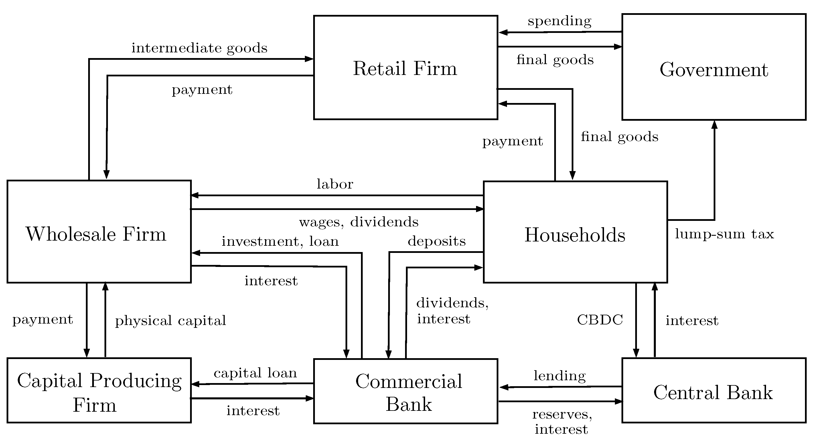
3. The Model Economy

We follow the standard framework of DSGE modeling to assess the macroeconomic consequences of introducing an interest-bearing CBDC, especially we want to know how the cash will compete with CBDC with respect to their prices and transaction costs. In this section, we outline the economy of our model and expose the optimization problems solved by households and firms. We also describe the behavior of financial intermediaries by commercial bank and the monetary and fiscal authorities by the central bank and the government.

3.1. Assumptions

Our model economy is populated by seven classes of agents: a continuum of identical households of measure unity indexed by $h\in [0,1]$, a retail firm or final-good producing firm, a continuum of wholesale firms or intermediate-good producing firms indexed by $j\in [0,1]$, a capital-producing firm, commercial banks, the central bank as a monetary authority and the government as a fiscal authority. In a representative agent model, identical agents in household and firm sectors mean that all agents differ, but they act in such a way that the sum of their preferences is mathematically equivalent to the decision of one representative agent.

The basic structure of our DSGE model is depicted in Figure 1. The model is built according to the closed economy New Keynesian framework by [8,43,44]. Households consume and supply labor to wholesale firms, receive wages, choose the real levels of cash, deposits, and CBDC to hold at the beginning of the period, and pay lump-sum tax to the government. As the owners, households also receive dividends from firms and commercial banks. Retail firm aggregates imperfectly substitutable intermediate goods into a single final good, which is used for consumption, investment, or government spending. The final good is sold at a perfectly competitive price. Wholesale firms use the labor provided by households and capital to produce a unique good that is sold on the monopolistically competitive market. Wages are fully flexible and adjust to clear the market. Capital-producing firm purchases the final good for investment and combines it with existing capital stock to produce new capital goods. Commercial bank is owned by households. The bank supplies credit to wholesale firms to finance their short-term working capital needs, supplies credit to the capital-producing firm for investment financing, pays interest on household deposits and central bank loans, and holds minimum reserves against deposits at the central bank without remuneration. The central bank regulates the commercial bank and sets its policy interest rate using a Taylor-type rule and supplies all the credit demanded by the bank at the prevailing refinance rate. The government issues bonds, receives tax payments, and makes spending.

In some respects, we follow approaches developed in previous studies by others and in different standpoints we make few extensions. Our model has the following features:

1.

We consider a money-in-utility (MIU) intertemporal welfare function to be maximized by households [10,11]. The presence of cash in addition to bank deposits and CBDC is slightly extend the one by Gross & Schiller [8]. The cash also appears in the budget constraint.

2.

In the profit maximization of wholesale firms, we adopt the so-called Calvo price setting mechanism, where firms have a certain probability of either keeping the price fixed in the next period or optimally determining the price [12].

3.

Similar to [8,13], the nominal interest rate on CBDC follows the interest rate of central bank funding considering the financial stress expressed as the percentage deviation of banks’ equity from steady state. This rule is intended to disincentivize CBDC accumulation in a crisis.

4.

Government bonds are held by banks and the central bank.

5.

To quantify the effect of disruptions by economic shocks, our model is equipped with three shock generators, namely productivity shock, liquidity demand shock, and the monetary policy shock.

3.2. Households

In this model, the economy is populated by a continuum of households indexed by $h\in [0,1]$ whose problem is to maximize a particular intertemporal welfare function. To this end, a money-in-utility function proposed by Sidrauski [10] and in the form of the constant relative risk aversion (CRRA) utility function is adopted. The lifetime utility function $U^H$ is additively separable into consumption of goods $C_{h,t}$, supply of working hours $L_{h,t}$, and saving in the form of bank deposits $D_{h,t}$, money holding in cash (real money balance) $M_{h,t}$, and digital money holding in CBDC $E_{h,t}$. Each household h wants to maximize the following expected utility:

$$U^H={\mathbb{E}}_0\sum _{i=0}^{\infty }{\beta }^i\left(\begin{array}{c}{\displaystyle \frac{C_{h,i}^{1-\sigma }}{1-\sigma }+\frac{{\alpha }_e}{1-{\eta }_e}{\left(\frac{E_{h,i}}{P_i}\right)}^{1-{\eta }_e}+\frac{{\alpha }_m}{1-{\eta }_m}{\left(\frac{M_{h,i}}{P_i}\right)}^{1-{\eta }_m}}\\ {\displaystyle +\frac{{\alpha }_d}{1-{\eta }_d}{\left(\frac{D_{h,i}}{P_i}\right)}^{1-{\eta }_d}+\frac{{\alpha }_l{L}_{h,i}^{1+\phi }}{1+\phi }}\end{array}\right),$$

(1)

where ${\mathbb{E}}_0$ stands for the rational expectation operator conditional on the information set at time zero. In (1), CBDC, cash, and deposits are expressed in nominal values as they are weighted by the price level $P_i$, $\beta \in (0,1)$ is the intertemporal discount factor, $\sigma \in (0,1)$ is the relative risk aversion coefficient, ${\alpha }_e,{\alpha }_m,{\alpha }_d>0$ are relative utility weights or preference parameters of CBDC, cash, and bank deposits, respectively, $\phi$ is coefficient relates to Frisch elasticity of labor supply, and ${\eta }_e,{\eta }_m,{\eta }_d>0$ are coefficients relate to elasticity of bank deposits, cash, and CBDC. Note that we may extend the form of household’s utility function by introducing wealth in the form of government bonds $B_{h,i}^H$ as discussed by, for instance, Michaillat & Saez [45]. However, this extension modifies the properties of the New Keynesian IS curve, where the interest rate is now negatively related to output instead of being constant, equal to the time discount rate.

Households are assumed to consume goods, invest money, pay taxes, and receive wages for their labor supplied. Households also own the firms and the banks, and therefore receive dividends and profits sharing. Decisions made by households in maximizing (1) must satisfy the following budget constraint:

$$\begin{array}{c}{P}_t(C_{h,t}+IN{V}_{h,t})+E_{h,t}+M_{h,t}+D_{h,t}+TA{X}_{h,t}=W_t{L}_{h,t}+R_t^K{K}_{h,t}\hfill \\ \hfill +(1+I_{t-1}^E)E_{h,t-1}+M_{h,t-1}+(1+I_{t-1}^D)D_{h,t-1}+{\mathrm{\Pi }}_{h,t}^{FB}.\end{array}$$

(2)

The terms on the left-hand side of (2) summarize the use of economic resources by households, and those on the right-hand side indicate the economic resources. $IN{V}_{h,t}$ is level of investment, $TA{X}_{h,t}$ is the lump sum tax, $W_t$ is the level of wages, $K_{h,t}$ is the capital stock, $R_t^K$ is the return on capital, $I_t^E$ is the nominal interest rate of CBDC, $I_t^D$ is the nominal interest rate of bank deposits, and ${\mathrm{\Pi }}_{h,t}^{FB}$ is the profit (dividend) from firms and banks. An additional equation represents the capital stock dynamics is:

$$K_{h,t+1}=IN{V}_{h,t}+(1-\delta )K_{h,t},$$

(3)

where $\delta$ is the depreciation rate of physical capital.

Lifetime utility (1) maximization, with respect to $C_{h,t}$, $L_{h,t}$, $K_{h,t}$, $E_{h,t}$, $M_{h,t}$, and $D_{h,t}$, subject to budget constraint (2) and capital stock (3) yields the following first order conditions:

$$\begin{array}{cc}\hfill {\alpha }_l{C}_t^{\sigma }{L}_t^{\phi }& =\frac{W_t}{P_t},\hfill \end{array}$$

(4)

$$\begin{array}{cc}\hfill {\left(\frac{{\mathbb{E}}_t{C}_{t+1}}{C_t}\right)}^{\sigma }& =\beta \left(1-\delta +{\mathbb{E}}_t\frac{R_{t+1}^K}{P_{t+1}}\right),\hfill \end{array}$$

(5)

$$\begin{array}{cc}\hfill {\alpha }_e{\left(\frac{E_t}{P_t}\right)}^{-{\eta }_e}& =\frac{C_t^{-\sigma }}{P_t}-\beta (1+I_t^E){\mathbb{E}}_t\frac{C_{t+1}^{-\sigma }}{P_{t+1}},\hfill \end{array}$$

(6)

$$\begin{array}{cc}\hfill {\alpha }_m{\left(\frac{M_t}{P_t}\right)}^{-{\eta }_m}& =\frac{C_t^{-\sigma }}{P_t}-\beta {\mathbb{E}}_t\frac{C_{t+1}^{-\sigma }}{P_{t+1}},\hfill \end{array}$$

(7)

$$\begin{array}{cc}\hfill {\alpha }_d{\left(\frac{D_t}{P_t}\right)}^{-{\eta }_d}& =\frac{C_t^{-\sigma }}{P_t}-\beta (1+I_t^D){\mathbb{E}}_t\frac{C_{t+1}^{-\sigma }}{P_{t+1}}.\hfill \end{array}$$

(8)

Note that derivation processes allow us to drop the index h from variables. The complete proofs for (4)–(8) can be found in Appendix B.

Under transaction costs of using cash and CBDC, the total consumption can be decomposed as follows:

$$C_t=C_t^M(1+S\left(v_t^M\right))+C_t^E(1+S\left(v_t^E\right)),$$

(9)

where $S\left(v_t^M\right)$ and $S\left(v_t^E\right)$ are the transaction costs of using cash and CBDC, respectively, as functions of money velocities $v_t^M$ and $v_t^E$, while $C_t^M$ and $C_t^E$ are the consumption levels using cash and CBDC. The money velocities with respect to cash and CBDC are, respectively, given by:

$$\begin{array}{cc}\hfill v_t^M& =\frac{C_t^M}{M_t},\hfill \end{array}$$

(10)

$$\begin{array}{cc}\hfill v_t^E& =\frac{C_t^E}{E_t}.\hfill \end{array}$$

(11)

In this work, we adopt transaction cost functions proposed by Schmitt-Grohe & Uribe [46] as follows:

$$S\left(v_t\right)=a{v}_t+\frac{b}{v_t}-2\sqrt{ab},$$

(12)

where a and b are all positive cost parameters. Cost function S has a satiation level of velocity $v^{*}=\sqrt{b/a}$. We can easily verify that S is decreasing when $v_t<v^{*}$ and increasing when $v_t>v^{*}$. The transaction cost functions for cash and CBDC are given by:

$$\begin{array}{cc}\hfill S_t^M& =Z_t^M{a}_M\frac{C_t^M}{M_t}+b_M\frac{M_t}{C_t^M}-2\sqrt{a_M{b}_M},\hfill \end{array}$$

(13)

$$\begin{array}{cc}\hfill S_t^E& =Z_t^E{a}_E\frac{C_t^E}{E_t}+b_E\frac{E_t}{C_t^E}-2\sqrt{a_E{b}_E},\hfill \end{array}$$

(14)

where we denote $S_t^M=S\left(v_t^M\right)$ and $S_t^E=S\left(v_t^E\right)$, while $Z_t^M$ and $Z_t^E$ are the shocks on the demand for total liquidities in term of cash and CBDC, respectively, which follow first order autoregressive processes:

$$\begin{array}{cc}\hfill ln{Z}_t^M& ={\rho }_{M}ln{Z}_{t-1}^M+{\epsilon }_t^M,\hfill \end{array}$$

(15)

$$\begin{array}{cc}\hfill ln{Z}_t^E& ={\rho }_{E}ln{Z}_{t-1}^E-{\epsilon }_t^E,\hfill \end{array}$$

(16)

where ${\rho }_M,{\rho }_E\in (0,1)$ are the degree of persistence in the cash and CBDC demands, and ${\epsilon }_t^M\sim N(0,{\sigma }_M)$ and ${\epsilon }_t^E\sim N(0,{\sigma }_E)$ are the errors. As pointed out by [38], an increase in $S_t^M$ or $S_t^E$ can be considered as a flight to safety, meaning a higher demand for liquid assets for a given volume of real economic transactions. CBDC that has cheaper transaction cost than cash will have smaller parameters values, i.e., $a_E\le a_M$ and $b_E\le b_M$.

Further, consumption levels by using cash and CBDC are given by:

$$\begin{array}{cc}\hfill C_t^M& ={\left(\frac{P_t^M}{P_t}\right)}^{-\zeta }{C}_t,\hfill \end{array}$$

(17)

$$\begin{array}{cc}\hfill C_t^E& ={\left(\frac{P_t^E}{P_t}\right)}^{-\zeta }{C}_t,\hfill \end{array}$$

(18)

where $\zeta$ is the elasticity of substitution between cash and CBDC payments for consumption, $P_t^M$ and $P_t^E$ are the prices of goods by using cash and CBDC, respectively, and they govern the general price:

$$P_t={({\left(P_t^M\right)}^{1-\zeta }+{\left(P_t^E\right)}^{1-\zeta })}^{\frac{1}{1-\zeta }}.$$

(19)

The proofs for (17)–(19) are provided in Appendix C.

3.3. Retail Firms

Suppose that at time t wholesale firm j produces $Y_{j,t}$ units of intermediate good and there are a continuum of intermediate goods over the unit interval $[0,1]$. These intermediate goods are CES aggregated by a retail firm (final good producer) to produce $Y_t$. The production technology for assembling intermediate goods to produce the final good is given by the standard Dixit-Stiglitz technology [47]:

$$Y_t={\left({\int }_0^1{\left(Y_{j,t}\right)}^{\frac{\theta -1}{\theta }}dj\right)}^{\frac{\theta }{\theta -1}},$$

(20)

where $\theta >1$ represents the elasticity of substitution between intermediate goods. With the nominal price of a final good being denoted by $P_t$ and that of a intermediate good j denoted by $P_{j,t}$, the price of each intermediate good is taken as a given by retail firms. Therefore, the representative retail firm chooses the quantities of intermediate goods such that maximize its profits:

$$U^{RF}=P_t{Y}_t-{\int }_0^1{P}_{j,t}{Y}_{j,t}dj,$$

(21)

where the first term in (21) is the total revenue from selling final goods and the second term is the total cost of buying intermediate goods. Substituting the aggregator technology (20) leads to the following first order condition of profit maximization:

$$Y_{j,t}={\left(\frac{P_{j,t}}{P_t}\right)}^{-\theta }{Y}_t.$$

(22)

Equation (22) accounts the demand level of intermediate good j, which is directly proportional to aggregate demand $Y_t$ and inversely proportional to its relative price level $P_t$.

3.4. Wholesale Firms

Each wholesale firm j produces a perishable intermediate good that is sold on a monopolistically competitive market. To produce these goods, each firm rents capital at the price $R_t$ from the capital good producer and combines it with labor from households. To produce the output $Y_t$, each wholesale firm has a Cobb–Douglas production function:

$$Y_{j,t}=A_t{K}_{j,t}^{\alpha }{L}_{j,t}^{1-\alpha },$$

(23)

where $K_{j,t}$ is the amount of capital rented by wholesale firm j from capital market, $L_{j,t}$ is the number of working hours supplied by households to firm j, $\alpha \in (0,1)$ is the elasticity of output with respect to capital, and $A_t$ is the productivity shock, a variable that can be interpreted as the level of general knowledge about the arts of production available in an economy. It is assumed that productivity shocks follow a first-order autoregressive process, such that:

$$ln{A}_t={\rho }_{A}ln{A}_{t-1}+{\epsilon }_t^A,$$

(24)

where ${\rho }_A\in (-1,1)$ is the degree of persistence of the shock and ${\epsilon }_t^A\sim N(0,{\sigma }_A)$ is the error.

Total wages should be transferred by wholesale firm j to household is $W_t{L}_{j,t}$. However, we assume that there is a possibility wholesale firm j can take a loan from commercial bank to pay some part of wages in advance. The amount of the loan for this purpose, denoted by $Q_{j,t}^{IF}$, is given by:

$$Q_{j,t}^{IF}=k_Q{W}_t{L}_{j,t},$$

(25)

where $k_Q\in (0,1)$ is the portion of total wages borrowed from bank. In [44], $k_Q$ represents the strength of the cost channel. As we may write $W_t{L}_{j,t}=Q_{j,t}^{IF}+(1-k_Q)W_t{L}_{j,t}$ and since it is assumed that short-term loans for working capital do not carry any risk and are therefore contracted at a rate that reflects only the marginal cost of borrowing from the central bank, $I_t^{CB}$, which is the refinance rate [44], then the wages claim faced by the wholesale firm is given by:

$$(1+I_t^{CB})Q_{j,t}^{IF}+(1-k_Q)W_t{L}_{j,t}=(1+k_Q{I}_t^{CB})W_t{L}_{j,t}.$$

(26)

3.4.1. The Cost Minimization Problem

The wholesale firm solves a two-stage optimization problem. First, the firm j takes the prices of the factors of production (return on capital $R_t^K$ and wages $W_t$) as given and determines the amount of capital and labor that it will use to minimize its total production cost. The total cost $T{C}_{j,t}$ to be minimized by the firm consists of wages bill (26) and capital rent:

$$T{C}_{j,t}=(1+k_Q{R}_t^L)W_t{L}_{j,t}+R_t^K{K}_{j,t},$$

(27)

subject to production function (23). The corresponding Lagrange function for this problem is:

$${\mathcal{L}}^{IF}=(1+k_Q{I}_t^{CB})W_t{L}_{j,t}+R_t^K{K}_{j,t}+{\mathrm{\Lambda }}_t^{IF}(Y_{j,t}-A_t{K}_{j,t}^a{L}_{j,t}^{1-a}),$$

(28)

where ${\mathrm{\Lambda }}_t^{IF}$ is the Lagrange multiplier. The first order condition with respect to $L_{j,t}$ and $K_{j,t}$ are, respectively, as follow:

$$\begin{array}{cc}\hfill (1+k_Q{I}_t^{CB})W_t-(1-\alpha ){\mathrm{\Lambda }}_t^{IF}{A}_t{K}_{j,t}^{\alpha }{L}_{j,t}^{-\alpha }& =0,\hfill \\ \hfill R_t^K-\alpha {\mathrm{\Lambda }}_t^{IF}{A}_t{K}_{j,t}^{\alpha -1}{L}_{j,t}^{1-\alpha }& =0.\hfill \end{array}$$

From the second condition, we have:

$$\frac{R_t^K{K}_{j,t}}{\alpha L_{j,t}}={\mathrm{\Lambda }}_t^{IF}{A}_t{K}_{j,t}^{\alpha }{L}_{j,t}^{-\alpha },$$

and substitution to the first condition provides:

$$\frac{K_{j,t}}{L_{j,t}}=\frac{\alpha (1+k_Q{I}_t^{CB})}{1-\alpha }\frac{W_t}{R_t^K}.$$

(29)

Since none of the terms on the right hand side of (29) depend on j, then the capital-labor ratio will be the same across all firms.

From (29) we may express $K_t$ as:

$$K_t=\frac{\alpha (1+k_Q{I}_t^{CB})}{1-\alpha }\frac{W_t}{R_t^K}{L}_t.$$

(30)

By substituting (30) into total cost (27) we obtain:

$$T{C}_t=\frac{1+k_Q{I}_t^{CB}}{1-\alpha }{W}_t{L}_t,$$

(31)

and by substituting (30) into production function (23) we get:

$$Y_t=A_t{\left(\frac{\alpha (1+k_Q{I}_t^{CB})}{1-\alpha }\frac{W_t}{R_t^K}\right)}^{\alpha }{L}_t,$$

or equivalently:

$$L_t=\frac{Y_t}{A_t}{\left(\frac{\alpha (1+k_Q{I}_t^{CB})}{1-\alpha }\frac{W_t}{R_t^K}\right)}^{-\alpha }.$$

(32)

Substitution (32) into the total optimal cost function (31) yields:

$$T{C}_t=\frac{Y_t}{A_t}{\left(\frac{(1+k_Q{I}_t^{CB})W_t}{1-\alpha }\right)}^{1-\alpha }{\left(\frac{R_t^K}{\alpha }\right)}^{\alpha }.$$

(33)

Finally, the marginal cost function $M{C}_t$ is the derivative of the total cost function (33) with respect to $Y_t$:

$$M{C}_t=\frac{1}{A_t}{\left(\frac{(1+k_Q{I}_t^{CB})W_t}{1-\alpha }\right)}^{1-\alpha }{\left(\frac{R_t^K}{\alpha }\right)}^{\alpha }.$$

(34)

Subsequently, we can rewrite $L_t$ in (32) and $K_t$ in (30) in term of $M{C}_t$, respectively, as follow:

$$\begin{array}{cc}\hfill L_t& =\frac{1-\alpha }{1+k_Q{I}_t^{CB}}M{C}_t\frac{Y_t}{W_t},\hfill \end{array}$$

(35)

$$\begin{array}{cc}\hfill K_t& =\alpha M{C}_t\frac{Y_t}{R_t^K}.\hfill \end{array}$$

(36)

3.4.2. The Profit Maximization Problem

In the second stage, wholesale firm wants to maximize the real profits it gives back to households. Since the real marginal cost is the optimal cost of producing one unit of goods, the firm’s problem is to maximize:

$${\mathrm{\Pi }}_{j,t}^{IF}=P_{j,t}{Y}_{j,t}-M{C}_t{Y}_{j,t}.$$

(37)

In addition to the stochastic discount factor $\beta$, firms will also discount their future profits by $\varphi$. We also impose that the wholesale firms face the constraint that they can only adjust prices following a Calvo-type rule. The wholesale firm has a $\varphi$ probability of keeping the price fixed in the next period and a $1-\varphi$ probability of optimally determining its price. Hence, a wholesale firm wants to maximize:

$${\mathrm{\Pi }}_{j,t}^{IF}={\mathbb{E}}_t\sum _{s=0}^{\infty }{\left(\beta \varphi \right)}^s(P_{j,t}{Y}_{j,t+s}-M{C}_{t+s}{Y}_{j,t+s}),$$

(38)

subject to production constraint (22), which is adjusted as:

$$Y_{j,t+s}={\left(\frac{P_{t+s}}{P_{j,t}}\right)}^{\theta }{Y}_{t+s}.$$

(39)

Substitution the optimal production constraint (39) into profit function (38) gives:

$${\mathrm{\Pi }}_{j,t}^{IF}={\mathbb{E}}_t\sum _{s=0}^{\infty }{\left(\beta \varphi \right)}^s(P_{j,t}^{1-\theta }{P}_{t+s}^{\theta }-P_{j,t}^{-\theta }{P}_{t+s}^{\theta }M{C}_{t+s})Y_{t+s}.$$

(40)

The first order condition with respect to $P_{j,t}$ is then given by:

$${\mathbb{E}}_t\sum _{s=0}^{\infty }{\left(\beta \varphi \right)}^s((1-\theta )P_{j,t}^{-\theta }{P}_{t+s}^{\theta -1}+\theta P_{j,t}^{-\theta -1}{P}_{t+s}^{\theta -1}M{C}_{t+s})Y_{t+s}=0,$$

(41)

or equivalently:

$${\mathbb{E}}_t\sum _{s=0}^{\infty }{\left(\beta \varphi \right)}^s\left(1+\frac{\theta }{1-\theta }\frac{M{C}_{t+s}}{P_{j,t}}\right)=0.$$

(42)

We may proceed (42) to have:

$$\begin{array}{cc}\hfill \sum _{s=0}^{\infty }{\left(\beta \varphi \right)}^s& =\frac{\theta }{1-\theta }{\mathbb{E}}_t\sum _{s=0}^{\infty }{\left(\beta \varphi \right)}^s\frac{M{C}_{t+s}}{P_{j,t}}\hfill \\ \hfill \frac{P_{j,t}}{1-\beta \varphi }& =\frac{\theta }{1-\theta }{\mathbb{E}}_t\sum _{s=0}^{\infty }{\left(\beta \varphi \right)}^{s}M{C}_{t+s}\hfill \\ \hfill P_{j,t}& =\frac{\theta (1-\beta \varphi )}{1-\theta }{\mathbb{E}}_t\sum _{s=0}^{\infty }{\left(\beta \varphi \right)}^{s}M{C}_{t+s}.\hfill \end{array}$$

Instead, we follow the approach adopted by Fernandez-Villaverde et al. [24] to proceed (41) such that we obtain:

$${\mathbb{E}}_t\sum _{s=0}^{\infty }{\left(\beta \varphi \right)}^s\left(\frac{1-\theta }{P_{j,t}}{\left(\frac{P_{j,t}}{P_{t+s}}\right)}^{1-\theta }+\frac{\theta }{P_{j,t}}{\left(\frac{P_{j,t}}{P_{t+s}}\right)}^{-\theta }\frac{M{C}_{t+s}}{P_{t+s}}\right)Y_{t+s}=0,$$

and then becomes:

$${\mathbb{E}}_t\sum _{s=0}^{\infty }{\left(\beta \varphi \right)}^s\left({\left(\frac{P_{j,t}}{P_{t+s}}\right)}^{1-\theta }+\frac{\theta }{1-\theta }{\left(\frac{P_{j,t}}{P_{t+s}}\right)}^{-\theta }\frac{M{C}_{t+s}}{P_{t+s}}\right)Y_{t+s}=0.$$

(43)

3.5. Capital Producing Firms

In the economy, all the capital is owned by the capital producing firm who adopts a linear production function to produce capital goods. At the beginning of the period, the capital producing firm buys $IN{V}_t$ of the final goods from the retail firm for investment purposes. Because payments for these final goods must be made in advance, the capital producing firms borrows $Q_t^{CF}$ from the commercial bank to purchase the capital. Thus,

$$Q_t^{CF}=IN{V}_t.$$

(44)

The loan in (44) must be paid in full plus interest with lending rate $I_t^L$. The capital producing firms then combines investment goods and the existing capital stock to create new capital goods $K_{t+1}$. The new capital stock is then rented to wholesale firms at the rate $R_t^K$. Recall that the dynamic of capital stocks is given in (3).

Taking the rental rate of capital $R_t^K$, the lending interest rate $I_t^L$, and the price of the final goods $P_t$ as given, the capital producing firm chooses the level of the capital stock so as to maximize the profits to the household. The real profits of the capital producing firm can be denoted as:

$${\mathrm{\Pi }}_t^{CF}=R_t^K{K}_t-(1+I_t^L)IN{V}_t,$$

(45)

and the value of the discounted stream of dividend payments to the household to be maximized is then formulated as:

$${\mathrm{\Pi }}^{CF}={\mathbb{E}}_t\sum _{t=0}^{\infty }{\beta }^t{\mathrm{\Lambda }}_t^H{\mathrm{\Pi }}_t^{CF},$$

(46)

where it is assumed, as in [44,48], that the capital producing firm values future profits according to the household’s intertemporal marginal rate of substitution in consumption ${\mathrm{\Lambda }}_t^H$, i.e., the Lagrange multiplier of households’ utility maximization given in (A35). This assumption is imposed because, in this model, the household and capital producing firm can be considered as a single unit with respect to housing choices.

From (3), we get $IN{V}_i=K_{i+1}-(1-\delta )K_i$, and by substituting it into (46) together with (45), we have the real profits function to be maximized:

$${\mathrm{\Pi }}^{CF}={\mathbb{E}}_t\sum _{i=0}^{\infty }{\beta }^i{\mathrm{\Lambda }}_i^H(R_i^K{K}_i-(1+I_i^L)(K_{i+1}-(1-\delta )K_i)).$$

By explicitly showing ${\mathrm{\Pi }}_t^{CF}$ at time t and $t+1$, we have:

$$\begin{array}{c}{\mathrm{\Pi }}^{CF}=\cdots +{\beta }^t{\mathrm{\Lambda }}_t^H(R_t^K{K}_t-(1+I_t^L)(K_{t+1}-(1-\delta )K_t))\hfill \\ \hfill {\beta }^{t+1}{\mathrm{\Lambda }}_{t+1}^H(R_{t+1}^K{K}_{t+1}-(1+I_{t+1}^L)(K_{t+2}-(1-\delta )K_{t+1}))+\cdots ,\end{array}$$

from which we obtain the first order condition with respect to $K_{t+1}$ as follows:

$$-{\mathrm{\Lambda }}_t^H(1+I_t^L)+\beta {\mathbb{E}}_t{\mathrm{\Lambda }}_{t+1}^H(R_{t+1}^K+(1-\delta )(1+I_{t+1}^L))=0.$$

Since ${\mathrm{\Lambda }}_t^H=-C_t^{-\sigma }/P_t$ from (A36), we then have:

$$\frac{C_t^{-\sigma }}{P_t}(1+I_t^L)=-\beta {\mathbb{E}}_t\frac{C_{t+1}^{-\sigma }}{P_{t+1}}(R_{t+1}^K+(1-\delta )(1+I_{t+1}^L)).$$

(47)

3.6. Banks

The commercial banks receive deposits $D_t$ from households at the beginning of each period. These deposits are managed by the banks to finance loans to wholesale firms for paying wages claim, which for a representative firm j it is $Q_{j,t}^{IF}$ in (25), and to the capital producing firm for investment $Q_t^{CF}$ in (44). Therefore, total lending $Q_t^B$ provided by the bank is:

$$Q_t^B=Q_t^{IF}+Q_t^{CF}=k_Q{W}_t{L}_t+IN{V}_t.$$

(48)

As refinancing via the central bank is more expensive than refinancing via deposits, i.e., $I_t^{CB}>I_t^D$, bank will only demand central bank funding to fill the gap between the supply of deposits $D_t$ and the maximum amount of total external lending $Q_t^B$. If the total lending is bigger than deposits, i.e., there is a shortfall in funding, bank borrows from the central bank $Q_t^{CB}$ with a net interest rate $I_t^{CB}$.

Bank’s liabilities comprise of loans from the central bank $Q_t^{CB}$, bank deposits $D_t$, and bank’s equity $N_t$, while bank’s assets consist of central bank reserves $T{R}_t$, loans to firms $Q_t^B$, and bonds $B_t^B$ as risk-free asset. Thus, the bank’s balance sheet is provided by:

$$Q_t^B+T{R}_t+B_t^B=Q_t^{CB}+D_t+N_t.$$

(49)

As total reserves $T{R}_t$ is a portion $\psi$ of deposit, i.e., $T{R}_t=\psi D_t$, and by (48), bank’s balance sheet (49) is then rewritten as:

$$Q_t^{IF}+Q_t^{CF}+B_t^B=Q_t^{CB}+(1-\psi )D_t+N_t.$$

(50)

Note that $N_t$ captures the bank’s equity, which is mainly driven by the interest rate premia. Since commercial bank lends their equity, households’ deposits, and funds from the central bank to the production sector, then the bank’s equity evolves according to the following equation:

$$N_{t+1}=(1+I_t^L)N_t+(I_t^L-I_t^D)D_t+(I_t^L-I_t^{CB})Q_t^{CB}.$$

(51)

In (51), $I_t^L-I_t^D$ and $I_t^L-I_t^{CB}$ denote the interest rate premia from deposits and central bank funds, respectively, by assuming that $I_t^L\ge I_t^D$ and $I_t^L\ge I_t^{CB}$.

The bank’s revenues come from equity $(1+I_t^L)N_t$, loans to wholesale firms $(1+I_t^{CB})Q_t^{IF}=k_Q(1+I_t^{CB})W_t{L}_t$, loans to capital production firms $(1+I_t^L)Q_t^{CF}=(1+I_t^L)IN{V}_t$, and bonds $(1+I_t^B)B_t^B$. Meanwhile, the bank’s liabilities come from deposits $(1+I_t^D)D_t$ and central bank loans $(1+I_t^{CB})Q_t^{CB}$. Therefore, the bank’s profit to be maximized is formulated as:

$$\begin{array}{c}{\mathrm{\Pi }}^B=(1+I_t^L)N_t+(1+I_t^{CB})Q_t^{IF}+(1+I_t^L)Q_t^{CF}+(1+I_t^B)B_t^B\hfill \\ \hfill -(1+I_t^D)D_t-(1+I_t^{CB})Q_t^{CB},\end{array}$$

(52)

subject to bank’s balance sheet (50). From (50), we may substitute $Q_t^{CB}$ as follows:

$$Q_t^{CB}=Q_t^{IF}+Q_t^{CF}+B_t^B-(1-\psi )D_t-N_t.$$

Thus, the bank’s profit (52) becomes:

$$\begin{array}{c}{\mathrm{\Pi }}^B=(1+I_t^L)N_t+(1+I_t^{CB})Q_t^{IF}+(1+I_t^L)Q_t^{CF}+(1+I_t^B)B_t^B\hfill \\ \hfill -(1+I_t^D)D_t-(1+I_t^{CB})(Q_t^{IF}+Q_t^{CF}+B_t^B-(1-\psi )D_t-N_t).\end{array}$$

(53)

The banks aim to determine the loan interest rate $I_t^L$ and the deposits interest rate $I_t^D$ in order to maximize their profit (53). Instead of maximizing (53) with respect to $I_t^L$ and $I_t^L$, it will be much easier differentiating (53) with respect to $(1+I_t^L)$ and $(1+I_t^D)$. Doing so, we respectively obtain:

$$\begin{array}{cc}\hfill N_t+Q_t^{CF}+(1+I_t^L)\frac{\partial Q_t^{CF}}{\partial (1+I_t^L)}-(1+I_t^{CB})\frac{\partial Q_t^{CF}}{\partial (1+I_t^L)}& =0,\hfill \end{array}$$

(54)

$$\begin{array}{cc}\hfill -D_t-(1+I_t^D)\frac{\partial D_t}{\partial (1+I_t^D)}+(1-\psi )(1+I_t^{CB})\frac{\partial D_t}{\partial (1+I_t^D)}& =0.\hfill \end{array}$$

(55)

We derive (54) and (55) by considering that $Q_t^{CF}$ is a function of $(1+I_t^L)$ and $D_t$ is a function of $(1+I_t^D)$. Next, we follow an approach in [44] by defining the coefficient of interest elasticity for loan supply to the wholesale firm ${\varphi }_L$ and that for deposits supply to households ${\varphi }_D$ as follows:

$$\begin{array}{cc}\hfill {\varphi }_L& =\frac{\partial Q_t^{CF}}{\partial (1+I_t^L)}\frac{1+I_t^L}{Q_t^{CF}},\hfill \end{array}$$

(56)

$$\begin{array}{cc}\hfill {\varphi }_D& =\frac{\partial D_t}{\partial (1+I_t^D)}\frac{1+I_t^D}{D_t}.\hfill \end{array}$$

(57)

Thus, by reformulating (54) and (55) in terms of ${\varphi }_L$ in (56) and ${\varphi }_D$ in (57), we obtain the optimal rates of loan and deposits:

$$\begin{array}{cc}\hfill 1+I_t^L& =\frac{{\varphi }_L(1+I_t^{CB})IN{V}_t}{N_t+(1+{\varphi }_L)IN{V}_t},\hfill \end{array}$$

(58)

$$\begin{array}{cc}\hfill 1+I_t^D& =\frac{{\varphi }_D(1-\psi )(1+I_t^{CB})}{1+{\varphi }_D}.\hfill \end{array}$$

(59)

It is shown in (58) and (59) that loan and deposit rates depend positively on refinance rate from the central bank $I_t^{CB}$. It is also known that $I_t^L$ depends negatively on the ratio of bank’s equity and investment $N_t/IN{V}_t$.

3.7. The Central Bank

While the rate of government bonds $I_t^B$ follows the interest rate on central bank funding $I_t^{CB}$ in the way that:

$$I_t^B=I_t^{CB}+{\mathrm{\Lambda }}^B,$$

(60)

where ${\Delta }^B>0$ is the fixed spread, the nominal interest rate on CBDC $I_t^E$ is set by the central bank. In the case of a non-interest-bearing CBDC, the central bank sets $I_t^E=0$. In order to use CBDC as a policy instrument, for an interest-bearing CBDC, the interest rate on CBDC strictly follows the interest rate on central bank funding with an individual rule-based determination, as suggested by Gross & Schiller [8]:

$$I_t^E=I_t^{CB}-\left({\Delta }^E+k_N\frac{\overline{N}-N_t}{\overline{N}}\right).$$

(61)

The terms in brackets in (61) define the spread between the interest rates on central bank funding $I_t^{CB}$ and that of CBDC $I_t^E$, where ${\Delta }^E>0$ is the fixed spread, and $N_t$ is the bank’s equity with steady state value $\overline{N}$. If $N_t$ is below its steady state value $\overline{N}$, then the spread increases, meaning that the CBDC rate is much lower than the central bank rate. In (61), the percentage deviation of banks’ equity from steady state $(\overline{N}-N_t)/\overline{N}$ represents the financial stress with $k_N\in (0,1)$ denotes the reaction intensity.

The central bank sets the policy interest rate on central bank funding $i_t^{CB}$ according to a Taylor-type rule. The policy rule is given in the following linear form:

$$I_t^{CB}={\rho }_R{I}_{t-1}^{CB}+(1-{\rho }_R)({\overline{R}}^B+{\pi }_t+{\varphi }_{\pi }({\pi }_t-{\pi }^T)+{\varphi }_y(Y_t-\overline{Y})+u_t,$$

(62)

where ${\rho }_R\in (0,1)$ is the interest rate smoothing parameter, ${\overline{R}}^B$ is the steady state value of the bonds interest rate, ${\pi }_t$ is the current inflation rate, ${\pi }^T$ is the central bank’s inflation target, $y_t$ is the output with steady state value $\overline{Y}$, ${\varphi }_{\pi }$ and ${\varphi }_y$ are, respectively, relative weights on inflation deviation and the output gap, and $u_t$ is the shock of first-order autoregressive process:

$$u_t={\rho }_u{u}_{t-1}+{\epsilon }_t^u,$$

(63)

where ${\rho }_u\in (-1,1)$ is the degree of persistence of the shock and ${\epsilon }_t^u\sim N(0,{\sigma }_u)$ is the error.

The central bank’s assets consist of government bonds holding $B_t^{CB}$, tax payment $TA{X}_t$, and loans to the commercial banks $Q_t^{CB}$, whereas its liabilities comprise total reserves $T{R}_t$ and currency supplied to households and firms in the forms of cash $M_t^S$ and CBDC $E_t^S$. The central bank’s balance sheet is thus formulated as:

$$(1+I_t^B)B_t^{CB}+TA{X}_t+(1+I_t^{CB})Q_t^{CB}=T{R}_t-T{R}_{t-1}+M_t^S+E_t^S.$$

(64)

Note that profits from bonds holding $I_t^B{B}_t^{CB}$ and from loan $I_t^{CB}{Q}_t^{CB}$ as well as lump sum tax $TA{X}_t$ are then transferred to the government. Since $T{R}_t=\psi D_t$ and currencies supplies can be given by $M_t^S=M_t-{\mu }_m{M}_{t-1}$ and $E_t^S=E_t-{\mu }_e{E}_{t-1}$ for cash and CBDC, respectively, then (64) becomes:

$$\begin{array}{c}(1+I_t^B)B_t^{CB}+TA{X}_t+(1+I_t^{CB})Q_t^{CB}=\psi (D_t-D_{t-1})\hfill \\ \hfill +(M_t-{\mu }_m{M}_{t-1})+(E_t-{\mu }_e{E}_{t-1}),\end{array}$$

(65)

where ${\mu }_m$ and ${\mu }_e$ are the measure of nominal rigidity in the money supply process.

3.8. The Government

In the economy, the government purchases the final good from retail firms $G_t$, collects taxes from households $TA{X}_t$, and issues one-period risk-free bonds $B_t$. The total bonds issued by government is given by:

$$B_t=B_t^B+B_t^{CB},$$

(66)

where $B_t^B$ are bonds held by commercial bank and $B_t^{CB}$ are those held by the central bank. The government’s budget constraint is formulated as:

$$P_t{G}_t+(1+I_{t-1}^B)B_{t-1}=TA{X}_t+B_t+I_t^{CB}{Q}_t^{CB}+I_t^B{B}_t^{CB},$$

(67)

where we assume that the profits earned by the central bank from loans and bonds holding are transferred to the government as fiscal authority. By (66), the budget constraint (67) becomes:

$$P_t{G}_t+(1+I_{t-1}^B)B_{t-1}^B+B_{t-1}^{CB}=TA{X}_t+B_t^B+(1+I_t^B)B_t^{CB}+I_t^{CB}{Q}_t^{CB}.$$

(68)

The government’s spending can be a constant fraction $k_G\in (0,1)$ of output of the final goods:

$$G_t=k_G{Y}_t,$$

(69)

and since output is divided into consumption, investment, and government spending, then the economy-wide budget constraint is expressed as:

$$Y_t=C_t+IN{V}_t+G_t.$$

(70)

4. Log-Linearization

One easy and common approach to solve and analyze DSGE models is to approximate the nonlinear equations characterizing the equilibrium with the corresponding log-linearized equations. The principle is to employ a first order Taylor approximation around a particular point (usually a steady state value) to replace the nonlinear equations with their approximations, which are linear in the log-deviations of the variables. In this work, we follow a log-linearization method proposed by Uhlig [49].

Let $X_t$ be the value of variable at time t and $\overline{X}$ be the steady state value of $X_t$. The log-linearized form of $X_t$, denoted by $x_t$, is defined as:

$$x_t=ln{X}_t-ln\overline{X}=ln\frac{X_t}{\overline{X}}.$$

(71)

Since the first order Taylor approximation of function $h=h\left(x\right)$ around $x=a$ is given by $h\left(x\right)\approx h\left(a\right)+h^{\prime }\left(a\right)(x-a)$, and thus for $h\left(X_t\right)=ln(X_t/\overline{X})$ we have $h^{\prime }\left(X_t\right)=1/X_t$, then the approximation of $X_t$ around its steady state value $\overline{X}$ in (71) is $x_t\approx (X_t-\overline{X})/\overline{X}$, from which we obtain the equivalency:

$$X_t\approx \overline{X}(1+x_t).$$

(72)

Alternatively, as from (71) we get $ln{X}_t=x_t+ln\overline{X}$, then by taking the exponent of both sides, we obtain $X_t\approx \overline{X}{e}^{x_t}$. By fact that Taylor approximation provides $e^{x_t}\approx 1+x_t$, then we again reclaim (72).

The nonlinear equations characterizing the equilibrium conditions of the model are presented in Section 3. The log-linearized version of these equations can be found in Appendix A.

5. Calibration

In this section, we examine the general equilibrium effects of the introduction of an interest-bearing CBDC on the macroeconomic. In particular, we inspect the effect of transaction costs, required reserves ratio, productivity shock, and monetary policy shock through impulse response functions. An illustrative calibration of the model is performed for Indonesia as a middle-income country. Other conventional parameters values are taken from relevant references.

The intertemporal discount factor is $\beta =0.985$, and the relative risk aversion coefficient is $\sigma =0.5$. Both values are in line with estimates for developing countries [44]. According to [8], elasticity coefficients of having CBDC, cash, and deposits are set to ${\eta }_e={\eta }_m={\eta }_d=0.95$. The relative utility weights or preference parameters of CBDCs, cash, and deposits are assigned to ${\alpha }_e={\alpha }_m={\alpha }_d=0.125$, while that of labor time is ${\alpha }_l=3.409$. The coefficient relates to Frisch elasticity of labor supply is $\phi =0.276$ [43].

In the production sector, as is standard in the literature, the depreciation rate of physical capital is $\delta =0.034$ and the elasticity of substitution between intermediate goods is $\theta =10$. The elasticity of output with respect to capital is set to be $\alpha =0.33$ as in [38]. These values are consistent with estimates for developing countries. The portion of total wages borrowed from bank, i.e., the strength of the cost channel, is taken to be $k_Q=0.75$ [44]. In price determination mechanism, we assume that there is a $\varphi =0.779$ probability of keeping the price fixed in the next period, and thus a $1-\varphi =0.221$ probability of optimally setting the price [43].

In banking sector, we assume that the constant interest elasticity of the supply of loan by the wholesale firm is ${\varphi }_L=-0.5$ and that of deposits by the household is ${\varphi }_D=0.5$. For the parameters related to the central bank, we use the values suggested by Chawwa [50] based on Indonesia aggregate banking data, the steady state value of required reserves ratio is $\psi =6.5$%, the government spending share is $k_G=9$%, following the average Indonesia government consumption relative to GDP, and the steady state value of the policy interest rate is ${\overline{R}}^B=1.8$%. For Taylor rule parameters, we use the conventional values of ${\varphi }_{\pi }=1.5$ for the feedback coefficient on inflation and ${\varphi }_y=0.5$ for the output gap coefficient, along with a value of ${\rho }_R=0.8$ for interest rate smoothing parameter [43]. According to Bank Indonesia, the inflation target is ${\pi }^T=3$%. The spread of bonds interest rate from central bank rate is assumed to be ${\mathrm{\Lambda }}^B=0.01$ and that of CBDC interest rate is ${\mathrm{\Lambda }}^E=0.005$ [8]. Beside a fixed spread, the dynamics of CBDC interest rate depends also on financial stress as expressed in (61). In this strategy, we set $k_N=0.01$ as the reaction intensity towards financial stress [8]. Based on [51], we specify the measure of nominal rigidity in cash and CBDC supply processes as ${\mu }_m={\mu }_e=1$. The degree of persistence in the monetary policy shock is set to be ${\rho }_u=0.74$ [52] and that of the productivity shock is ${\varphi }_A=0.97$ [53]. In the case of liquidity shocks, we assume ${\rho }_M=0.85$ and ${\rho }_E=0.9$.

The steady state value of all variables are simultaneously calculated based on steady state conditions derived from equations of motion in Appendix A. As initial values, we set $\overline{P}=1$, ${\overline{P}}^M=1/3$, $\overline{A}=1$, and ${\overline{I}}^{CB}=0.01$. Description and value of all parameters are summarized in

Table 1. The value of parameters.

No.	Parameter	Description	Value
1	$\beta$	intertemporal discount factor	$0.985$
2	$\sigma$	relative risk aversion coefficient	$0.5$
3	${\eta }_m$	elasticity of having cash	$0.95$
4	${\eta }_e$	elasticity of having CBDC	$0.95$
5	${\eta }_d$	elasticity of having bank deposits	$0.95$
6	$\phi$	coefficient relates to Frisch elasticity of labor supply	$0.276$
7	${\alpha }_m$	relative utility weights or preference parameters of cash	$0.1250$
8	${\alpha }_e$	relative utility weights or preference parameters of CBDC	$0.1250$
9	${\alpha }_d$	relative utility weights or preference parameters of bank deposits	$0.1250$
10	${\alpha }_l$	relative utility weights or preference parameters of labor time	$3.409$
11	${\rho }_M$	degree of persistence in cash demand shock	$0.85$
12	${\rho }_E$	degree of persistence in CBDC demand shock	$0.9$
13	$\delta$	depreciation rate of physical capital	$0.034$
14	$\theta$	elasticity of substitution between intermediate goods	10
15	$\alpha$	elasticity of output with respect to capital	$0.33$
16	${\rho }_A$	degree of persistence in the supply shock	$0.97$
17	$k_Q$	the portion of total wages borrowed from bank (strength of the cost channel)	$0.75$
18	$\varphi$	probability of keeping the price fixed in the next period	$0.779$
19	$1-\varphi$	probability of optimally determining the price	$0.221$
20	$\psi$	share of required reserves	$0.065$
21	${\varphi }_L$	constant interest elasticity of the supply of loan by the wholesale firm	$-0.5$
22	${\varphi }_D$	constant interest elasticity of the supply of deposits by the household	$0.5$
23	${\Delta }^B$	fixed spread of bonds interest rate from central bank rate	$0.01$
24	${\Delta }^E$	fixed spread of CBDC interest rate from central bank rate	$0.005$
25	$k_N$	reaction intensity towards financial stress	$0.01$
26	${\rho }_R$	interest rate smoothing parameter	$0.81$
27	${\overline{R}}^B$	steady state value of the policy interest rate	$0.018$
28	${\varphi }_{\pi }$	relative weights on inflation deviation	$1.5$
29	${\pi }^T$	inflation target	$0.03$
30	${\varphi }_y$	relative weights on output gap	$0.125$
31	${\rho }_u$	degree of persistence in the monetary policy shock	$0.74$
32	${\mu }_m$	measure of nominal rigidity in the cash supply process	1
33	${\mu }_e$	measure of nominal rigidity in the CBDC supply process	1

.

6. Policy Analysis

In this section, we present the simulation result of the model to explore the responses of variables with respect to liquidity demand shock, productivity shock, and monetary policy shock. We use Matlab Dynare to produce the impulse response functions with one period is a quarter.

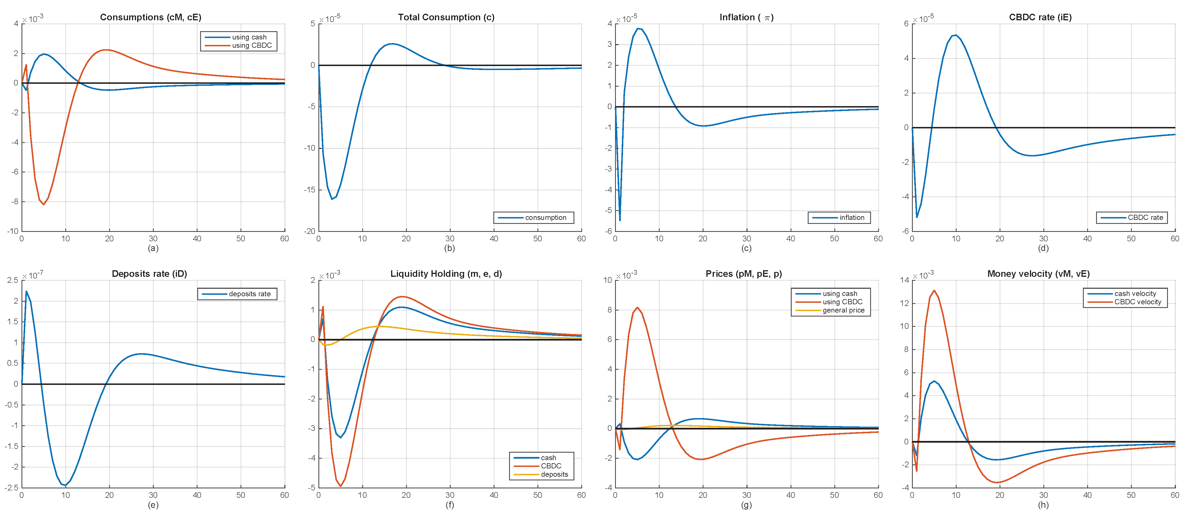
6.1. Effects of Liquidity Demand Shock

As stated in (9), consumptions by households are constrained by transaction cost. The cost is a function of money velocity with two parameters a and b as given in (13) and (14). Smaller a and b contributes cheaper transaction cost. However, the magnitude of the cost depends also on the types of money, where in our case is either cash or CBDC, whose velocities are determined by the model. To assess the effect of transaction costs, we specify the following cost parameters: $a_M=a_E=1$ and $b_M=b_E=1.5$. By this setting, we consider a situation where cash and CBDC have the same parameters values, and thus the same transaction cost provided the velocities of cash and CBDC are identical. In this simulation, we apply a negative shock on the transaction cost using CBDC as given in (14) to indicate that CBDC has a lower transaction cost.

Figure 2 shows the impact of negative shock of CBDC transaction cost on several relevant variables of the model. A negative shock is intended to decrease the transaction cost using CBDC by 1%. When the shock hits, consumption purchases using CBDC increase as the cost becomes cheaper, and consumption purchases using cash slightly decrease, see Figure 2a. However, in total, consumption purchases decrease. This fact informs us that households spend more CBDC in purchasing consumption goods, confirmed by a rise in CBDC demand as a response of shock in Figure 2f, even though the rate of CBDC is decreased by the shock as indicated by Figure 2d. In contrast to CBDC, the demand of bank deposits is decreasing even though its rate is increasing, see Figure 2e,f. From the perspective of price, a negative shock on CBDC cost is responded by a decrease in price of goods using CBDC $p_t^E$ in Figure 2g, which indicates that transaction using CBDC is cheaper than using cash. However, the general price $p_t$, which is aggregated from prices of cash and CBDC in (19), does not respond the shock very much as it fluctuates around its steady state value for all time. This small change in price is followed by a little drop in inflation rate, see Figure 2c. From the view point of money velocity, the negative shock of CBDC transaction cost is reacted by a decline in the velocity of CBDC as depicted by Figure 2h.

The simulation results presented in this section, however, indicate that the issuance of an interest-bearing CBDC has the potential to become a profitable means of liquidity storage and to have an impact that does not harm the economy.

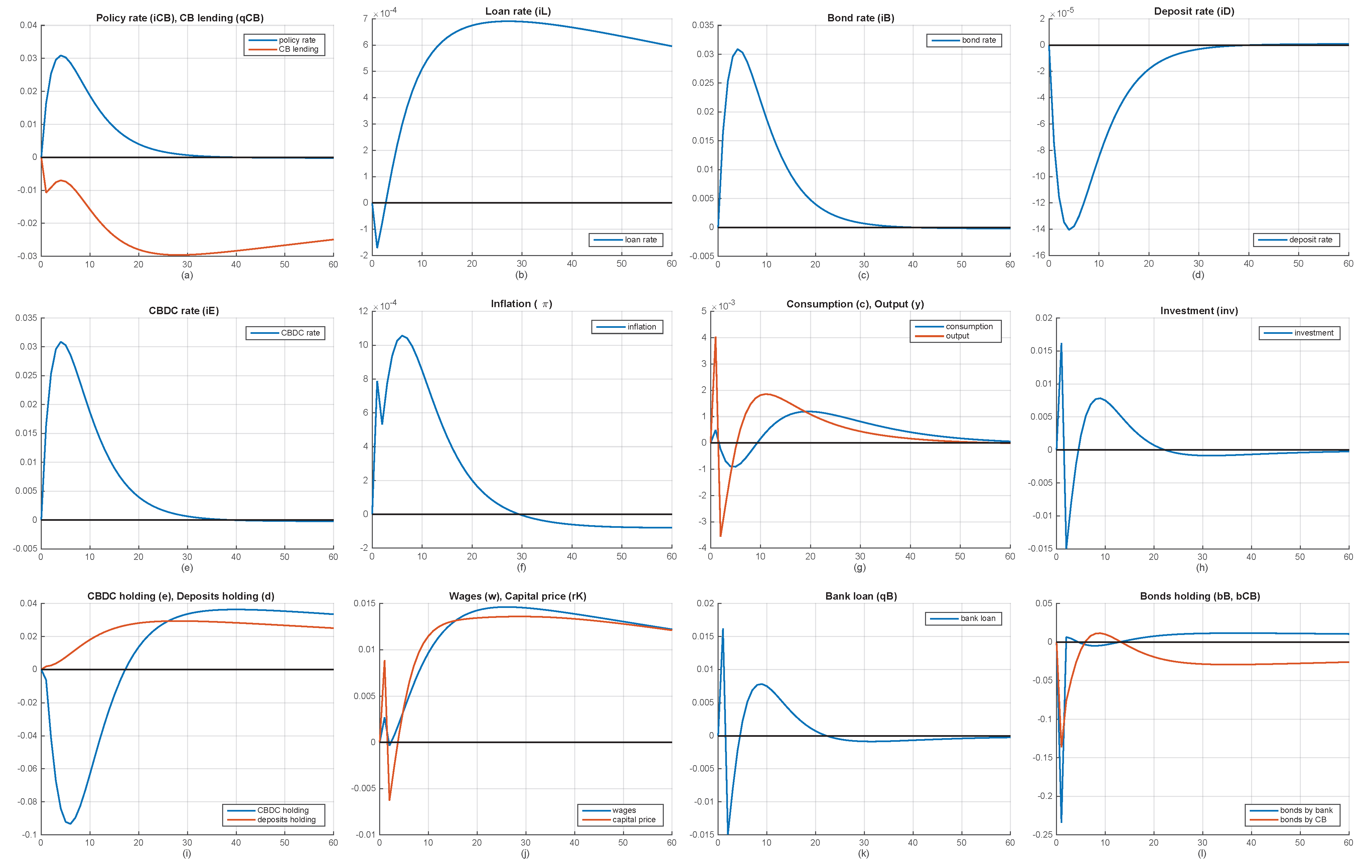
6.2. Effects of Productivity Shock

The effects of productivity shock on a number of main variables of the model are presented in Figure 3. The productivity shock due to the technological advance causes a rise in the values of the marginal products of labor and capital, and thus firms increase their demand for production inputs, so investment level increased. When one percent shock in productivity hits, the demand for labor increases more than 2% during the first two periods as depicted in Figure 3a. The intensity of labor declines quickly toward steady state. In the same figure, a similar hike in capital demand is shown, but with a more sloping rise and fall. Increasing productivity implies that firms produce more outputs (up to 3% hike), but operate more efficiently so the marginal costs decrease by about 2.5%, see Figure 3e.

Meanwhile, inflations slightly fall in the first ten periods as the production becomes more efficient, see Figure 3f. A small drop in inflation rate causes an increase in the supply of goods, thus leading to easing in monetary policy. A hike in goods production implies a rise in the wage and capital return as indicated by Figure 3b. Thus, households tend to use their time for consumption rather than saving, thus instantaneously decreasing the holding of cash, CBDC, and deposit about 1% as informed in Figure 3g. Due to the decline in inflation, the base policy rate which is governed by the Taylor rule also decreases. The lower base policy rate induces to a direct decrease in the central bank refinance rate, which in turn decreases the deposit and CBDC rates and thus the demand for bank deposits and interest bearing CBDCs.

Due to an increased aggregate supply of output, the price level decreased by more than 2%, see Figure 3h, followed by a small decrease in the inflation rate in the early periods. The central bank responds with a decline of its policy rate followed by CBDC and banks rates to make an economic contraction by reducing purchasing power. As the consequence, bank capital is decreasing due to the decreasing loans and increased liability due to the rising deposit rate. A decline of policy rate also implies the reduction of bond rate, thus central banks and banks buy more bonds, as depicted in Figure 3i. As the result, the rising interest rate makes consumption and investment decline. Both people and firms tend to save their money in CBDC rather than the deposit due to the CBDC attributes of being a risk-free asset. Decreasing consumption implies reduced firm productivity, thus reducing the wage of the labor, moreover, the technology starting to deteriorate as the technology keeps depreciating. As the sources of tax revenue decreased, see Figure 3d, government spending also decreased. In the end, the aggregate demand will be reduced, thus the output will also be declined.

These results aligned with [40,41]. Both of the results imply that CBDC would likely make monetary policy more effective. It can be seen by the response of the central bank towards inflation using CBDC rate is effective. Moreover, households show that remunerated CBDC is more attractive than bonds to fulfill their liquidity, so it enhances the monetary policy effectiveness.

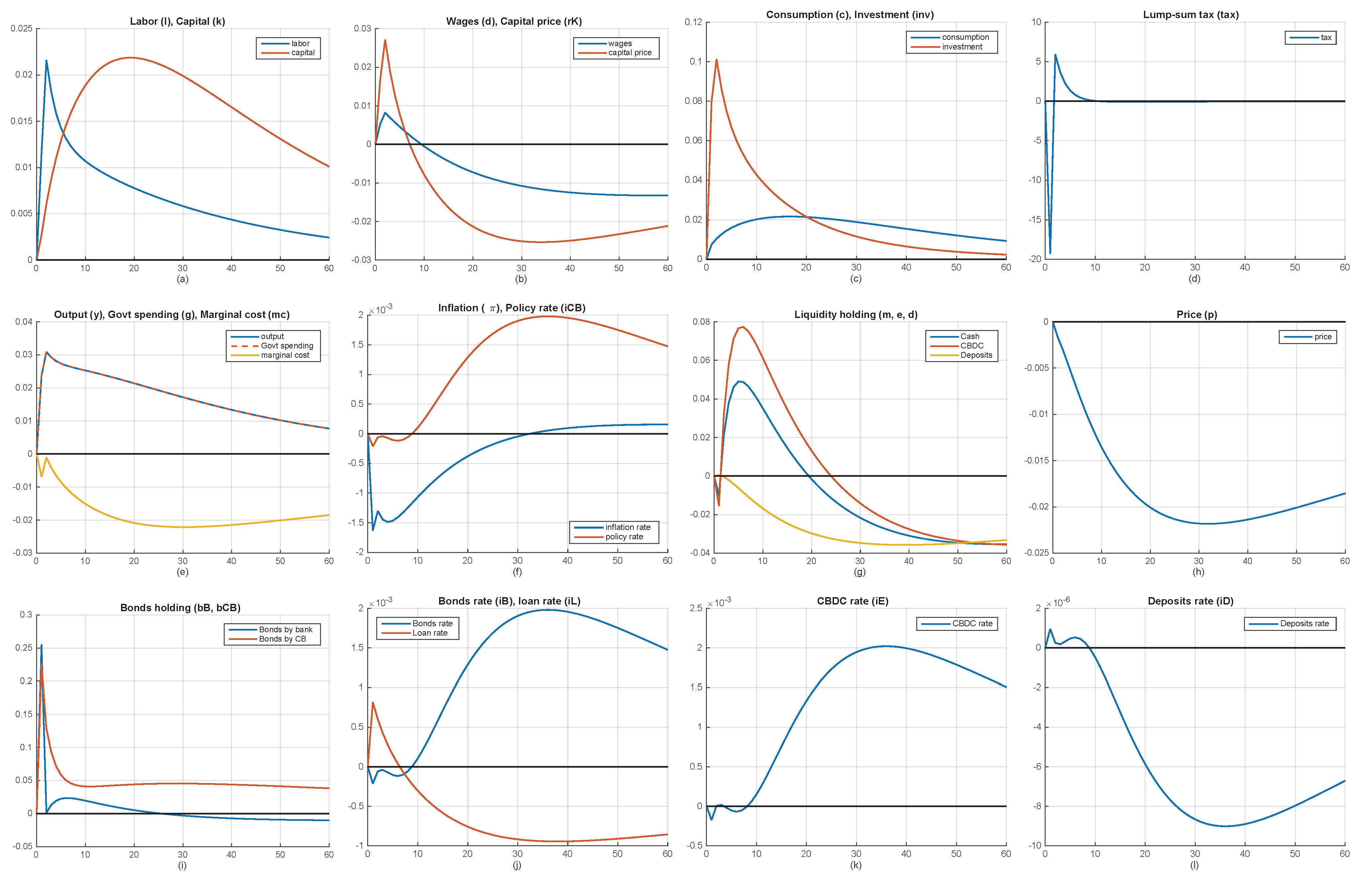
6.3. Effects of Monetary Policy Shock

Figure 4 depicts the effect of one percent increase in policy interest rate on several main variables of the model. A hike in policy rate means an increase of the borrowing cost from central bank, i.e., a decrease in funding provided by central bank. The dynamics of policy rate are mimicked by the bond rate and the CBDC rate as they are determined according to a fixed spread of the policy rate in (60) and (61). For CBDC, it is revealed that the financial stress term expressed in percentage deviation of banks’ equity from steady state gives no effect in this situation. A rise in policy rate is responded differently by the loan rate and deposits rate as they have to be determined optimally according to (58) and (59). The loan rate declines in the first period and increases in the half of remaining periods. While, the deposits rate declines during the first four periods, following by rises toward its steady state value.

The rise of CBDC rate immediately leads to the increase of CBDC demand and the fall of deposits rate directly causes the drop of bank deposits holding. However, the rise of bond rate is not followed by its demand. Bonds holding by bank and central bank drop by 23% and 13%, respectively, in response to monetary policy shock. These occurrences reveal a fact that households already consider CBDC as an alternative instrument of liquidity to bank deposits. Holding CBDC will increase the household’s overall liquidity, even though liquidity marginal utility decreased. Therefore, it is more explaining why CBDC is more attractive than the deposit. Since CBDC is remunerated, the households tend to convert more CBDC rather than cash or deposits.

There is lag in monetary policy transmission due to the cost adjustment of investment gradual response. In this lag period, households and firms tend to borrow money from bank to consume and invest before the bank done adjusting the interest rate, respectively. This lag explains why initially there is a short span increment in output when there is increment in the policy rate. After that period, households tend to substitute deposit to cash and CBDC due to the consideration of risk-free assets. CBDC also become an alternative to fulfill liquidity demand. The reduction of the deposit implies that banks have reduced credit supply, thus decreasing their lending power. As a result, there is a decrease in investment, which implies reduced labor as well as wages. Households also tend to save rather than take a loan. Reduced household and firm activity imply a reduction in purchasing power, thus reducing consumption as well as tax revenue. Due to the reduction in tax revenue, the government is also reducing its government spending. Reduced consumption and government spending also imply there is an excess supply of goods, which reduces the price level and inflation rate. Therefore, the reduction of aggregate demand reflects the reduction of output.

6.4. Implementation of the Analytical Model

Given the models in Section 3, it shows that CBDC involves many interactions among agents in the economy. Nonetheless, CBDC implementation itself brings both benefits and consequences [54]. On the high-level, CBDC could increase payment efficiency [55,56,57], monetary policy effectiveness [19,58,59], higher financial inclusion [60,61,62], and provide traceability [63,64,65]. This is also supported by the growing technology [66,67,68], network effect [17,69], the enthusiasm of CBDC [70,71,72], and cash inefficiency [73,74].

However, some consequences are the high cost of CBDC infrastructure [56,75], privacy loss potential [76,77], internet coverage limitation [62,78], and electrical outage [79,80]. This could be worsened by cyberattack threats [81,82], bank disintermediation amid crisis times [17], unprepared legal aspects [77,83], and private crypto-asset competitions [84,85,86].

Following the spirits of both CBDC benefits and consequences, we try to introduce some of the implications. First, CBDC implementation would likely increase budget spending due to its high cost of infrastructure and would disrupt innovation. Therefore, proposing a public–private partnership (PPP) allows us to maintain innovation, and also increase efficiency. The partnership could be with state-owned enterprises or private entities. Second, implementing CBDC implies that people could access their money 24/7, which means CBDC withdrawal could be conducted anytime/anywhere amid crisis times. One idea is to implement the capacity on the CBDC wallet, so there it could limit the withdrawal and will not create bank disintermediation. Third, implementing alternative offline payment (e.g., token-based offline CBDC) implies that people need to be aware of their private keys, otherwise they will lose access to their CBDC. To reduce the risk of losing the whole CBDC, the wallet could be limited so it will reduce the severity of losing CBDC. Fourth, implementing traceable CBDC implies that the central bank needs to govern the legal aspect consisting of the amount of extracted information, CBDC issuance, and eligible authority for CBDC operators. Those efforts are nothing but to maintain public trust. Fifth, central banks need to provide any means of backup plan to prevent a single point of failure risk. Preventing an outage is important because it could disrupt the whole financial system. Sixth, the central banks must use permissioned DLT to gain sufficient accessibility amid a decentralized system. Lastly, even though the central banks need to align their system to achieve interoperability in cross-border transactions, central banks still need to maintain their sovereignty.

7. Conclusions

The development of CBDC has been conducted by central banks across the world with various progress and motivation. From that consideration, implementing CBDC would likely to have macroeconomy consequences and monetary policy implication. However, it needs a comprehensive approach to support monetary policy based on those impacts. We have developed a medium size DSGE model to examine the interaction between CBDC and other variables and to quantify the macroeconomic effects of CBDC issuance. The proposed model consists of seven economic agents, namely households, retail firm, wholesale firms, capital producing firm, commercial bank, the central bank, and the government.

The model consider an economy in which the households may consider CBDC as a liquidity asset in addition to cash and bank deposits. The introduction of CBDC then differentiates the amount of consumption and the price in terms of cash and CBDC. As CBDC is designed to be an interest-bearing, CBDC may compete with cash in consumption process. The attractiveness of CBDC can also be appreciated at the lower transaction cost than cash. Thus, an interest-bearing CBDC can be considered as a profitable transaction instrument.

We have used the model to explain the main macroeconomic variables responses to a negative shock on CBDC transaction cost, as well as a positive supply shock, and a positive shock to the base policy rate. Our findings confirm that CBDC offers a number of macroeconomic benefits. A lower transaction cost offered by CBDC encourages households to consume more using CBDC, and thus reducing the purchase using cash. The price of goods counted in CBDC reduced, while the general price index is about in steady state leading to a small fall in inflation. As responses to an increase of output due to a productivity shock, we have shown that households use cash and CBDC in almost similar manners by reducing the holding for consumption. Responding to a one percent increase in the base policy rate, we have revealed that the dynamics of the policy interest rate is directly followed by that of CBDC. Thus, the accumulation of CBDC can be controlled by the policy rate.

As self-critical and possible limitations and shortcomings, our study considers only the issuance of retail CBDCs. More general situation in which commercial banks are enabled to provide loan to firms and to make settlement reserves in term of wholesale CBDCs will be the future research work. Additionally, the assessment of CBDC issuance in an open economy might be substantial to emerging countries as they have a significant portion of exports.

References

1. Pasuthip, P.; Yang, S. Central Bank Digital Currency: Promises and Risks; Academic Press: Cambridge, MA, USA, 2020. [Google Scholar]
2. Bank for International Settlements (BIS). COVID-19 Accelerated the Digitalisation of Payments; Committee on Payments and Market Infrastructures: Basel, Switzerland, 2021. [Google Scholar]
3. Balz, B. COVID-19 and cashless payments—Has coronavirus changed Europeans’ love of cash? In Proceedings of the Small and Medium Entrepreneurs Europe (SME Europe), Virtual Event, 21 October 2020. [Google Scholar]
4. Kotkowski, R.; Polasik, M. COVID-19 pandemic increases the divide between cash and cashless payment users in Europe. Econ. Lett. 2021, 209, 110139. [Google Scholar] [CrossRef] [PubMed]
5. Boar, C.; Holden, H.; Wadsworth, A. Impending Arrival—A Sequel to the Survey on Central Bank Digital Currency; BIS: Basel, Switzerland, 2020. [Google Scholar]
6. Klein, M.; Gross, J.; Sandner, P. The Digital Euro and the Role of DLT for Central Bank Digital Currencies; FSBC Working Paper; Frankfurt School Blockchain Center: Frankfurt, Germany, 2020. [Google Scholar]
7. Alonso, S.L.N.; Jorge-Vazquez, J.; Forradellas, R.F.R. Central banks digital currency: Detection of optimal countries for the implementation of a CBDC and the implication for payment industry open innovation. J. Open Innov. Technol. Mark. Complex. 2021, 7, 72. [Google Scholar] [CrossRef]
8. Gross, J.; Schiller, J. A model for central bank digital currencies: Implications for bank funding and monetary policy. SSRN Pap. 2021, 3721965, 1–46. [Google Scholar] [CrossRef]
9. Carapella, F.; Flemming, J. Central Bank Digital Currency: A Literature Review; FEDS Notes; Board of Governors of the Federal Reserve System: Washington, DC, USA, 2020. [Google Scholar]
10. Sidrauski, M. Rational choice and patterns of growth in a monetary economy. Am. Econ. Rev. 1967, 57, 534–544. [Google Scholar]
11. Blanchard, O.; Fischer, S. Lectures on Macroeconomics; MIT Press: Cambridge, MA, USA, 1989. [Google Scholar]
12. Calvo, G.A. Staggered prices in a utility-maximizing framework. J. Monet. Econ. 1983, 1, 383–398. [Google Scholar] [CrossRef]
13. Bindseil, U. Tiered CBDC and the Financial System; ECB Working Paper Series No. 2351; European Central Bank: Frankfurt, Germany, 2020. [Google Scholar]
14. Christiano, L.J.; Eichenbaum, M.; Evans, C.L. Nominal rigidities and the dynamic effects of a shock to monetary policy. J. Political Econ. 2005, 113, 1–45. [Google Scholar] [CrossRef] [Green Version]
15. Smets, F.; Wouters, R. Shocks and frictions in US business cycles: A bayesian DSGE approach. Am. Econ. Rev. 2007, 97, 586–606. [Google Scholar] [CrossRef] [Green Version]
16. Ferrari, M.M.; Mehl, A.; Stracca, L. Central Bank Digital Currency in an Open Economy; Working Paper No. 2488; European Central Bank: Frankfurt, Germany, 2020. [Google Scholar]
17. Agur, I.; Ari, A.; Dell’Ariccia, G. Designing central bank digital currencies. J. Monet. Econ. 2022, 125, 62–79. [Google Scholar] [CrossRef]
18. Andolfatto, D. Assessing the Impact of Central Bank Digital Currency on Private Banks; Working Paper 2018-026; Federal Reserve Bank of St. Louis: St. Louis, MO, USA, 2018. [Google Scholar]
19. Davoodalhosseini, S.M.R. Central Bank Digital Currency and Monetary Policy; Staff Working Paper 2018-36; Bank of Canada: Ottawa, ON, Canada, 2018. [Google Scholar]
20. Williamson, S.D. Central bank digital currency and flight to safety. J. Econ. Dyn. Control 2021, 104146, in press. [Google Scholar] [CrossRef]
21. Chiu, J.; Jiang, J.H.; Davoodalhosseini, S.M.R.; Zhu, Y. Central bank digital currency and banking. In Proceedings of the Society for Economic Dynamics: 2018 Annual Meeting of the Society for Economic Dynamics, Mexico City, Mexico, 28–30 June 2018. [Google Scholar]
22. Chiu, J.; Jiang, J.H.; Davoodalhosseini, S.M.R.; Zhu, Y. Bank Market Power and Central Bank Digital Currency: Theory and Quantitative Assessment; Staff Working Paper No. 2019-20; Bank of Canada: Ottawa, ON, Canada, 2020. [Google Scholar]
23. Keister, T.; Monnet, C. Central bank digital currency: Stability and information. In Proceedings of the 2018 Annual Research Conference of the Swiss National Bank and the Bank of Canada/Riksbank Conference on the Economics of Central Bank Digital Currencies, Ottawa, ON, Canada, 17–18 October 2019. [Google Scholar]
24. Fernandez-Villaverde, J.; Sanches, D.; Schilling, L.; Uhlig, H. Central bank digital currency: Central banking for all? Rev. Econ. Dyn. 2021, 41, 225–242. [Google Scholar] [CrossRef]
25. Kim, Y.S.; Kwon, O. Central Bank Digital Currency and Financial Stability; Working Paper; Bank of Korea: Seoul, Korea, 2019. [Google Scholar]
26. Bitter, L. Banking crises under a central bank digital currency (CBDC). In Beitrage zur Jahrestagung des Vereins fur Socialpolitik 2020: Gender Economics; ZBW—Leibniz Information Centre for Economics: Kiel, Germany, 2020. [Google Scholar]
27. Skeie, D.R. Digital Currency Runs; Chief Economists Workshop; Bank of England: London, UK, 2020. [Google Scholar]
28. Christiano, L.J.; Eichenbaum, M.S.; Trabandt, M. On DSGE models. J. Econ. Perspect. 2018, 32, 113–140. [Google Scholar] [CrossRef] [Green Version]
29. Stiglitz, J.E. Where modern macroeconomics went wrong. Oxf. Rev. Econ. Policy 2018, 24, 70–106. [Google Scholar] [CrossRef]
30. Vines, D.; Wills, S. The rebuilding macroeconomic theory project: An analytical assessment. Oxf. Rev. Econ. Policy 2018, 34, 1–42. [Google Scholar] [CrossRef]
31. Blanchard, O. PB 16-11 Do DSGE Models Have a Future? Peterson Institute for International Economics Policy Brief. August 2016, pp. 1–4. Available online: https://www.piie.com/system/files/documents/pb16-11.pdf (accessed on 28 April 2022).
32. Hurtado, S. DSGE models and the Lucas critique. Econ. Model. 2014, 44, S12–S19. [Google Scholar] [CrossRef] [Green Version]
33. Hoffmann, A. An overinvestment cycle in Central and Eastern Europe? Metroeconomica 2010, 61, 711–734. [Google Scholar] [CrossRef] [Green Version]
34. Hoffmann, A.; Schnabl, G. A vicious cycle of manias, crises and asymmetric policy responses—An overinvestment view. World Econ. 2011, 34, 382–403. [Google Scholar] [CrossRef] [Green Version]
35. Hoffmann, A.; Schnabl, G. National Monetary Policy, International Economic Instability and Feeback Effects—An Overinvestment View; Working Papers on Global Financial Markets No. 19; Universität Halle-Wittenberg: Halle, Germany, 2011. [Google Scholar]
36. Ghironi, F. Macro needs micro. Oxf. Rev. Econ. Policy 2018, 34, 195–218. [Google Scholar] [CrossRef]
37. Linde, J. DSGE models: Still useful in policy analysis? Oxf. Rev. Econ. Policy 2018, 34, 269–286. [Google Scholar] [CrossRef]
38. Barrdear, J.; Kumhof, M. The macroeconomics of central bank digital currencies. J. Econ. Dyn. Control 2021, 104148, in press. [Google Scholar] [CrossRef]
39. Luo, S.; Zhou, G.; Zhou, J. The impact of electronic money on monetary policy: Based on DSGE model simulations. Mathematics 2021, 9, 2614. [Google Scholar] [CrossRef]
40. Lim, K.Y.; Liu, C.; Zhang, S. Optimal Central Banking Policies: Envisioning the Post-Digital Yuan Economy with Loan Prime Rate-Setting; Discussion Papers in Economics No. 2021/2; Nottingham Trent University: Nottingham, UK, 2021. [Google Scholar]
41. George, A.; Xie, T.; Alba, J.D. Central Bank Digital Currency with Adjustable Interest Rate in Small Open Economies; Policy Research Paper No. 05-2020; Asia Competitiveness Institute, National University of Singapore: Singapore, 2020. [Google Scholar]
42. Benigno, P.; Schilling, L.M.; Uhlig, H. Cryptocurrencies, Currency Competition, and the Impossible Trinity; NBER Working Papers 26214; National Bureau of Economic Research: Cambridge, MA, USA, 2019. [Google Scholar] [CrossRef]
43. Gertler, M.; Karadi, P. A model of unconventional monetary policy. J. Monet. Econ. 2011, 58, 17–34. [Google Scholar] [CrossRef]
44. Primus, K. Excess reserves, monetary policy and financial volatility. J. Bank. Financ. 2017, 74, 153–168. [Google Scholar] [CrossRef] [Green Version]
45. Michaillat, P.; Saez, E. Resolving New Keynesian anomalies with wealth in the utility function. Rev. Econ. Stat. 2018, 103, 197–215. [Google Scholar] [CrossRef] [Green Version]
46. Schmitt-Grohe, S.; Uribe, M. Foreign demand for domestic currency and the optimal rate of inflation. J. Money Credit. Bank. 2012, 44, 1207–1224. [Google Scholar] [CrossRef]
47. Dixit, A.K.; Stiglitz, J.E. Monopolistic competition and optimum product diversity. Am. Econ. Rev. 1977, 67, 297–308. [Google Scholar]
48. Agenor, P.-R.; Alper, K.; da Silva, L.P. Capital regulation, monetary policy, and financial stability. Int. J. Cent. Bank. 2013, 9, 198–243. [Google Scholar]
49. Uhlig, H. A toolkit for analysing nonlinear dynamic stochastic models easily. In Computational Methods for the Study of Dynamic Economies; Marimon, R., Scott, A., Eds.; Oxford University Press: New York, NY, USA, 1999; pp. 30–61. [Google Scholar]
50. Chawwa, T. Impact of reserve requirement and liquidity coverage ratio: A DSGE model for Indonesia. Econ. Anal. Policy 2021, 71, 321–341. [Google Scholar] [CrossRef]
51. Piazzesi, M.; Rogers, C.; Schneider, M. Money and banking in a New Keynesian model. Bank of Canada Annual Conference—The Future of Money and Payments: Implications for Central Banking, Canada, ON, USA, 5–7 November 2020. [Google Scholar]
52. Harmanta; Purwanto, N.M.A.; Rachmanto, A.; Oktiyanto, F. Monetary and macroprudential policy mix under financial frictions mechanism with DSGE model. In Proceedings of the International Economic Modeling Conference 2014 (EcoMod 2014), Bali, Indonesia, 16–18 July 2014; pp. 1–35. [Google Scholar]
53. Angelini, P.; Neri, S.; Panetta, F. The interaction between capital requirements and monetary policy. J. Money Credit. Bank. 2014, 46, 1073–1112. [Google Scholar] [CrossRef]
54. Syarifuddin, F. Optimal Central Bank Digital Currency (CBDC) Design for Emerging Economies; Working Paper; Bank Indonesia Institute: Jakarta, Indonesia, 2022. [Google Scholar]
55. Bordo, M.; Levin, A. Central Bank Digital Currency and the Future of Monetary Policy; NBER Working Paper No. 23711; National Bureau of Economic Research: Cambridge, MA, USA, 2017. [Google Scholar]
56. CPMI. Central Bank Digital Currencies; Markets Committee Paper No. 174; BIS: Basel, Switzerland, 2018; pp. 1–34. [Google Scholar]
57. He, D.; Leckow, R.; Haksar, V.; Griffoli, T.; Jenkinson, N.; Kashima, M.; Khiaonarong, T.; Rochon, C.; Tourpe, H. Fintech and Financial Services: Initial Considerations; IMF Staff Discussion Notes No. 17/05; IMF: Washington, DC, USA, 2017. [Google Scholar]
58. Agur, I.; Bernaga, M.; Bordo, M.; Engert, W.; Lis, S.; Fung, B.; Gnan, E.; Levin, A.; Niepelt, D.; Judson, R.; et al. Do we need central bank digital currency? In Proceedings of the SUERF—The European Money and Finance Forum and BAFFI CAREFIN Centre, Bocconi University, Milan, Italy, 7 June 2018. [Google Scholar]
59. Nelson, B. The Benefits and Costs of a Central Bank Digital Currency for Monetary Policy; BPI Research Paper No. 202.589.2454; BSI: Basel, Switzerland, 2021. [Google Scholar]
60. Mersch, Y. An ECB digital currency—A flight of fancy? In Proceedings of the Consensus 2020 Virtual Conference, New York, NY, USA, 11–13 May 2020. [Google Scholar]
61. Wallis, J. Unlocking Financial Inclusion with CBDCs. Ripple Insight. 2021. Available online: https://ripple.com/insights/unlocking-financial-inclusion-with-cbdcs/ (accessed on 28 April 2022).
62. Didenko, A.N.; Buckley, R.P. Central Bank Digital Currencies: A Potential Response to the Financial Inclusion Challenges of the Pacific; Issues in Pacicif Development No. 3; Asian Development Bank: Mandaluyong, Philippines, 2021; pp. 1–40. [Google Scholar]
63. Nathan, A.; Galbraith, G.L.; Grimberg, J.; Bhushan, S.; Cahill, M.; Courvalin, D.; Pandl, Z.; Rosenberg, I.; Struyven, D.; Tilton, A.; et al. What’s in Store for the dollar. Goldman Sachs, 10 November 2020; 26p. [Google Scholar]
64. Adam-Kalfon, P.; Arslanian, H.; Sok, K.; Sureau, B.; Jones, H.; Dou, Y. PwC CBDC Global Index, 1st ed.; PwC: London, UK, 2021. [Google Scholar]
65. Mookerjee, A. What if central banks issued digital currency? Harvard Business Review, 15 October 2021; 1–11. [Google Scholar]
66. Adrian, T. Stablecoins, central bank digital currencies, and cross-border payments: A new look at the international monetary system. In International Monetary Fund; 14 May 2019; pp. 1–5. [Google Scholar]
67. An, Y.; Choi, P.; Huang, S. Blockchain, Cryptocurrency, and Artificial Intelligence in Finance; Springer: Singapore, 2021. [Google Scholar] [CrossRef]
68. People’s Bank of China (PBoC). Progress of Research & Development of E-CNY in China. Working Group on E-CNY Research and Development; People’s Bank of China: Hong-Kong, China, 2021. [Google Scholar]
69. Forner, G. Network Effects on Central Bank Digital Currencies and Blockchain Protocol Based Ledgers; Universita Ca’ Foscari Venezia: Venezia, Italy, 2020; Available online: http://hdl.handle.net/10579/17133 (accessed on 28 April 2022).
70. Boar, C.; Wehrli, A. Ready, Steady, Go?—Results of the Third BIS Survey on Central Bank Digital Currency; BIS Papers No. 114; BIS: Basel, Switzerland, 2021; pp. 77–82. [Google Scholar]
71. Gross, J.; Sedlmeir, J.; Babel, M.; Bechtel, A. Designing a Central Bank Digital Currency with Support for Cash-like Privacy; SSRN Papers No. 3891121; BIS: Basel, Switzerland, 2021. [Google Scholar]
72. Vives, X. Digital disruption in banking. Annu. Rev. Financ. Econ. 2019, 11, 243–272. [Google Scholar] [CrossRef]
73. Brugge, J.; Denecker, O.; Jawaid, H.; Kovacs, A.; Shami, I. Attacking the Cost of Cash; McKinsey & Company: Chicago, IL, USA, 2018; Available online: https://www.mckinsey.com/industries/financial-services/our-insights/attacking-the-cost-of-cash (accessed on 28 April 2022).
74. ING Group. Central Bank Digital Currency in a European Context. ING, 2020 17 August 2020. [Google Scholar]
75. Adrian, T.; Mancini-Griffoli, T. Central bank digital currencies: 4 questions and answers. IMF Blog, 12 December 2019. [Google Scholar]
76. Borgonovo, E.; Caselli, S.; Cillo, A.; Masciandaro, D.; Rabitti, G. Central Bank Digital Currencies, Crypto Currencies, and Anonymity: Economics and Experiments; SUERF Policy Brief No. 222; SUERF: Wien, Austria, 2021. [Google Scholar]
77. Jiang, J.; Lucero, K. Background and Implications of China’s Central Bank Digital Currency: E-CNY; SSRN Papers No. 3774479; Elservier: Amsterdam, The Netherlands, 2021. [Google Scholar]
78. Shah, D.; Arora, R.; Du, H.; Darbha, S.; Miedema, J.; Minwalla, C. Technology Approach for a CBDC; Bank of Canada: Ottawa, ON, Canada, 25 February 2020. [Google Scholar] [CrossRef]
79. Spivey, J. Technology Downtime: What’S Reasonable? (and What Isn’T?). WorkWingSwept Blog. 23 July 2021. Available online: https://www.wingswept.com/technology-downtime-whats-reasonable-and-what-isnt/ (accessed on 28 April 2022).
80. Wadsworth, A. The pros and cons of issuing a central bank digital currency. Reserv. Bank N. Z. Bull. 2018, 8, 1–21. [Google Scholar]
81. Auer, R.; Bohme, R. The technology of retail central bank digital currency. In BIS Quarterly Review; 1 March 2020; pp. 85–100. [Google Scholar]
82. Minwalla, C. Security of a CBDC; Bank of Canada: Ottawa, ON, Canada, 24 June 2020. [Google Scholar] [CrossRef]
83. Sveriges Riksbank. E-Krona Pilot Phase 1; Sveriges Riksbank Report; Sveriges Riksbank: Stockholm, Sweden, 2021; pp. 1–21. [Google Scholar]
84. Agur, I. Central bank digital currencies: An overview of pros and cons. In Proceedings of the SUERF—The European Money and Finance Forum and BAFFI CAREFIN Centre Bocconi University, Milan, Italy, 7 June 2018; pp. 121–132. [Google Scholar]
85. Goodell, G.; Aste, T. Can cryptocurrencies preserve privacy and comply with regulations? Front. Blockchain 2019, 2, 4. [Google Scholar] [CrossRef] [Green Version]
86. Morales-Resendiz, R.; Ponce, J.; Picardo, P.; Velasco, A.; Chen, B.; Sanz, L.; Guiborg, G.; Segendorff, B.; Vasquez, J.L.; Arroyo, J.; et al. Implementing a retail CBDC: Lessons learned and key insights. Lat. Am. J. Cent. Bank. 2021, 2, 100022. [Google Scholar] [CrossRef]
Figure 1. The model structure.
Mathematics 10 01671 g001
Figure 2. The effect of negative shock of CBDC transaction cost on (a) consumption by using cash c t M and CBDC c t E , (b) total consumption c t , (c) inflation π t , (d) CBDC rate i t E , (e) deposits rate i t D , (f) liquidity holding m t , e t , d t , (g) prices p t M , p t E , p t , and (h) money velocity v t M = c t M m t and v t E = c t E e t .
Mathematics 10 01671 g002
Figure 3. The effect of productivity shock on: (a) Labor l t and capital k t , (b) wages w t and price of capital r t K , (c) consumption c t and investment i n v t , (d) lump-sum tax t a x t , (e) output y t , government spending g t , and marginal cost m c t , (f) inflation π t and policy rate i t C B , (g) liquidity holding m t , e t , d t , (h) price p t , (i) bonds holding b t B , b t C B , (j) bond rate i t B and loan rate i t L , (k) CBDC rate i t E , and (l) deposits rate i t D .
Mathematics 10 01671 g003
Figure 4. The effect of monetary policy shock on: (a) Policy rate i t C B and central bank lending q t C B , (b) loan rate i t L , (c) bond rate i t B , (d) deposit rate i t D , (e) CBDC rate i t E , (f) inflation π t , (g) consumption c t and output y t , (h) investment i n v t , (i) CBDC holding e t and deposits d t , (j) wages w t and price of capital r t K , (k) bank’s loan q t B , and (l) bonds holding b t B , b t C B .
Mathematics 10 01671 g004