
Dynamics of Oxygen-Plankton Model with Variable Zooplankton Search Rate in Deterministic and Fluctuating Environments


Abstract
:1. Introduction
2. Construction of Basic Model
- The term describes the rate of oxygen production per unit of phytoplankton biomass during the daytime by photosynthetic activity; and indicate the respiration of phytoplankton and zooplankton, respectively, and is the loss of oxygen due to natural depletion in a marine ecosystem.
- The term describes the growth of phytoplankton depending on the amount of available oxygen. The function is named as a modified Holling type II functional response, based on the premise that the zooplankton’s search rate is dependent on the biomass of phytoplankton, rather than being constant (for details, see [10,11]). Again, the consumed phytoplankton biomass is transformed into zooplankton biomass with an efficiency of , which depends on the oxygen concentration (zooplankton die due to insufficient oxygen).
- is a smooth function, and for .
- , i.e., H increases with p and , i.e., saturates at for a large prey population.
- , and . Therefore, has a unique positive root, and it changes sign from positive to negative at the unique inflection point. A graphical representation of and is presented in Figure 2.
3. Positivity and Uniform Boundedness
4. Existence of Equilibria of (1) with Stability Analysis
4.1. Equilibrium Points
- Trivial equilibrium point corresponding to depletion of oxygen and the extinction of plankton;
- Planer equilibrium point (zooplankton free), where , and is a positive root of the following equation:Here, , , , ,
- Interior (coexistence) equilibrium , where , , and can be obtained by solving the following system of equations using the software MATHEMATICA:
4.2. Local Stability
5. Local Bifurcations
5.1. Transcritical Bifurcation
5.2. Hopf-Bifurcation
- Case 1:Therefore,So, at , when .
- Case 2:So,So, at , when .∴, for and
6. Numerical Simulations
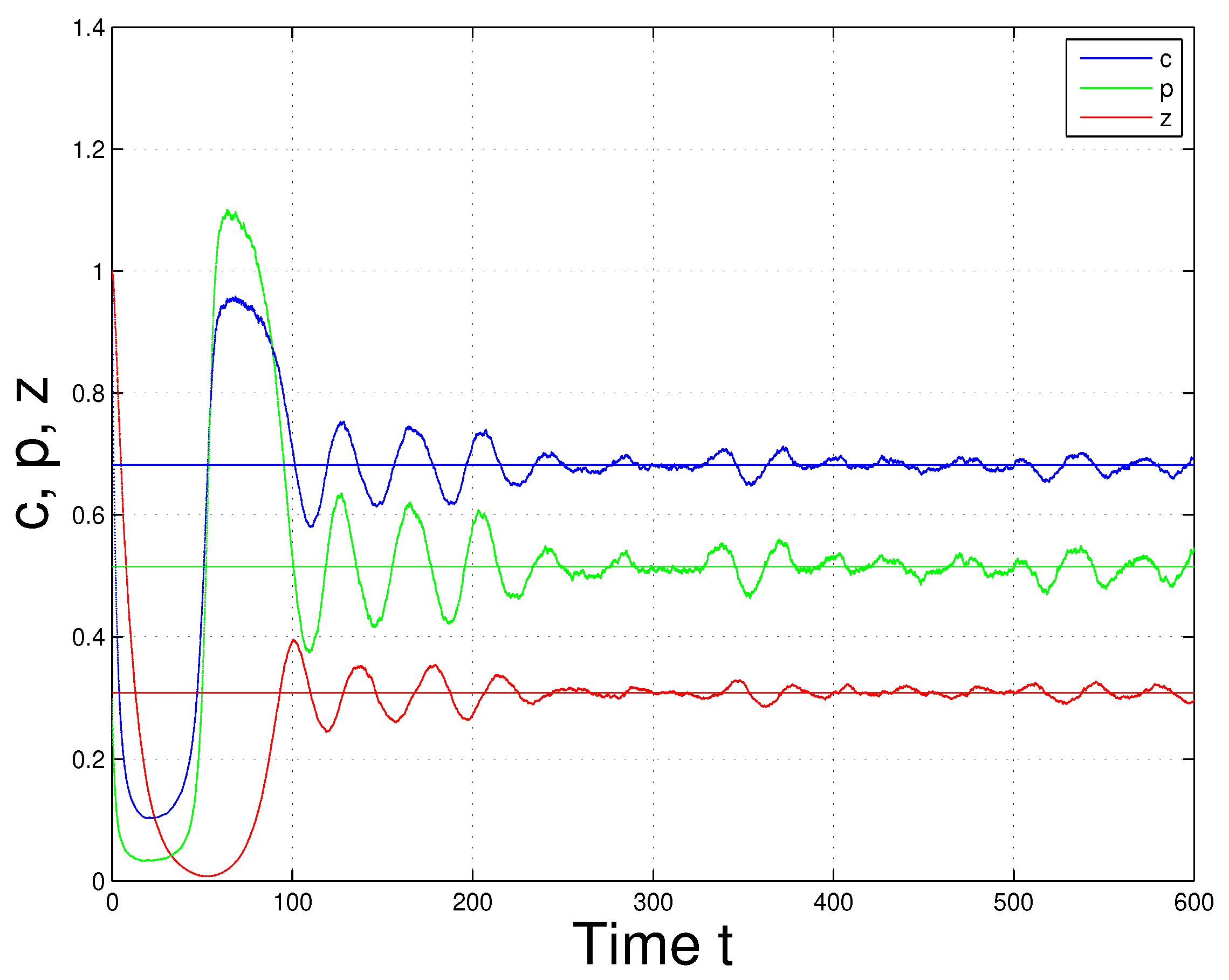
Effect of Environmental Noise on System (1)
7. Discussion and Conclusions
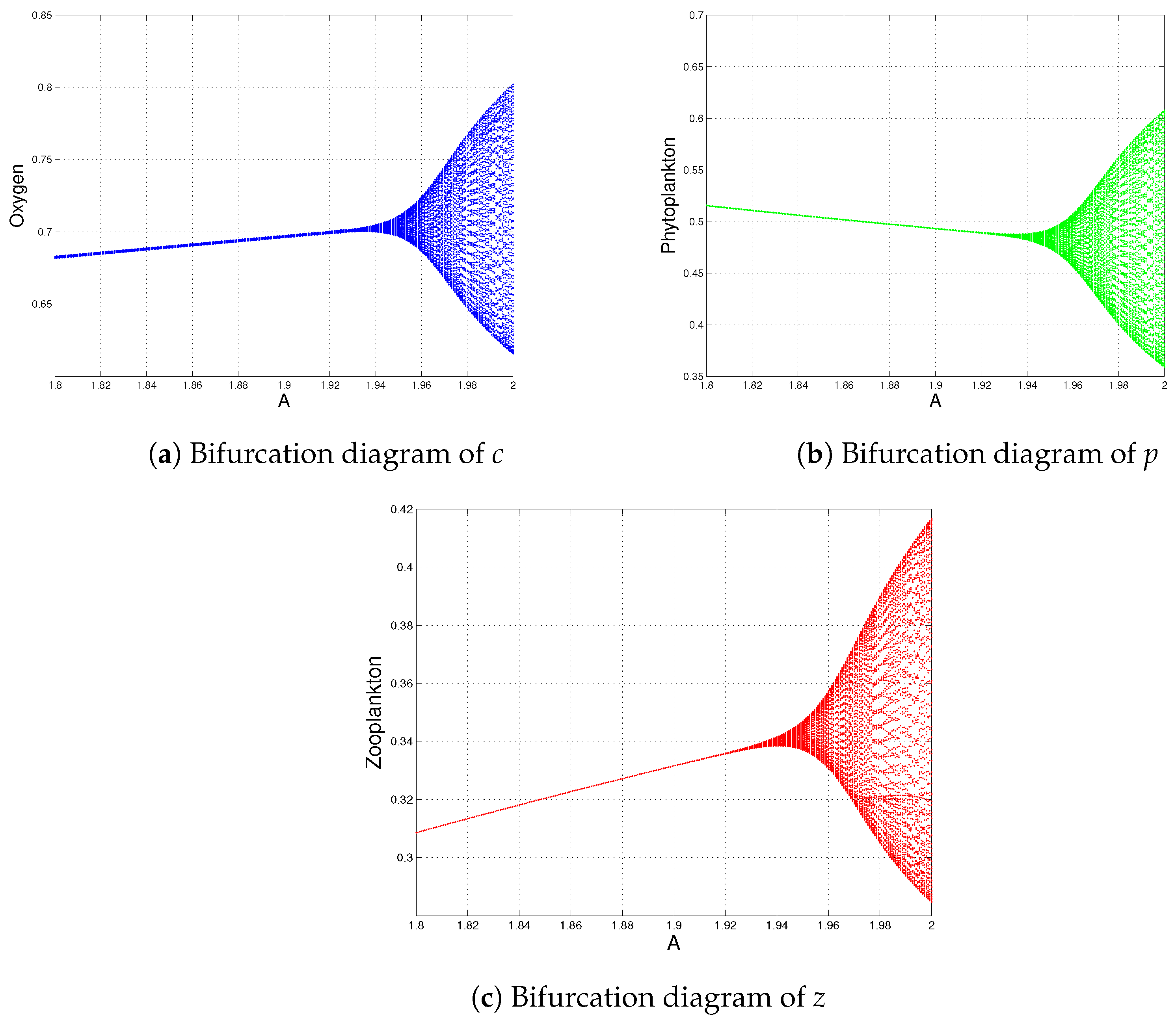
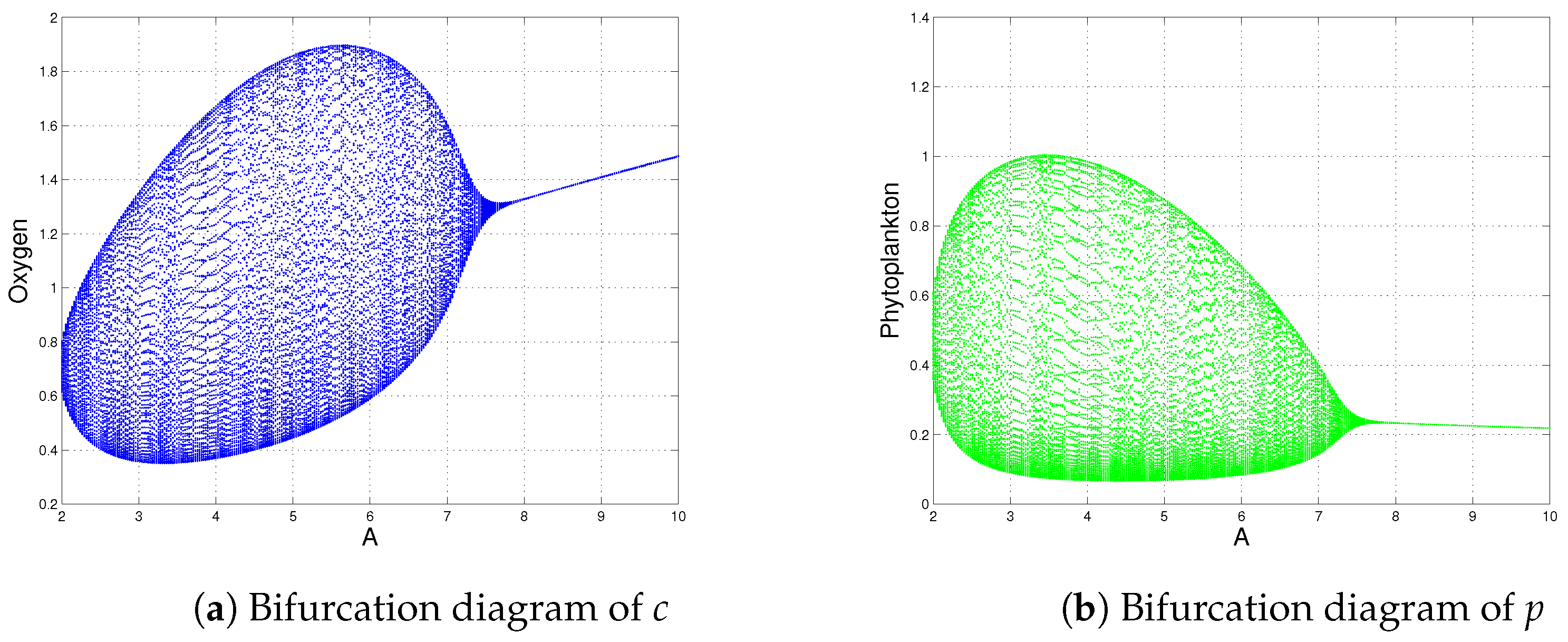
- System (1) always has a stable coexistence steady state for a high oxygen production rate (see Figure 6), i.e., the sustainability of oxygen production is possible when A is large (). This result is opposite to the outcome shown by Sekerci and Petrovskii [3] because they observed that the system dynamics were not sustainable for a high oxygen production rate. This is the main qualitative difference between the modified Holling type II (variable search rate, as mentioned in the proposed model) and the Holling type II functional responses. Therefore, the study of the modified Holling type II functional response is ecologically meaningful for the sustainability of the dynamics of system (1), if the net oxygen production rate is above a certain critical valve ().
Author Contributions
Funding
Institutional Review Board Statement
Informed Consent Statement
Data Availability Statement
Acknowledgments
Conflicts of Interest
References
- Harris, G.P. Phytoplankton Ecology: Structure, Function and Fluctuation; Springer: Dordrecht, The Netherlands, 1986. [Google Scholar]
- Moss, B.R. Ecology of Fresh Waters: Man and Medium, Past to Future; Wiley: London, UK, 2009. [Google Scholar]
- Sekerci, Y.; Petrovskii, S. Mathematical modelling of plankton-oxygen dynamics under the climate change. Bull. Math. Biol. 2015, 77, 2325–2353. [Google Scholar] [CrossRef] [PubMed] [Green Version]
- Gokce, A.; Yazar, S.; Sekerci, Y. Delay induced nonlinear dynamics of oxygen-plankton interactions. Chaos Solitons Fractals 2020, 141, 110327. [Google Scholar] [CrossRef]
- Sekerci, Y.; Petrovskii, S. Global Warming Can Lead to Depletion of Oxygen by Disrupting Phytoplankton Photosynthesis: A Mathematical Modelling Approach. Geosciences 2018, 8, 201. [Google Scholar] [CrossRef] [Green Version]
- Holling, C.S. The components of predation as revealed by a study of small-mammal predation of the european pine sawfly. Can. Entomol. 1959, 91, 293–320. [Google Scholar] [CrossRef]
- Holling, C.S. Some characteristics of simple types of predation and parasitism. Can. Entomol. 1959, 91, 385–398. [Google Scholar] [CrossRef]
- Holling, C.S. The functional response of predators to prey density and its role in mimicry and population regulation. Mem. Entomol. Soc. Can. 1965, 97 (Suppl. S45), 5–60. [Google Scholar] [CrossRef] [Green Version]
- Hassell, M.P.; Lawton, J.H.; Beddington, J.R. Sigmoid functional responses by invertebrate predators and parasitoids. J. Anim. Ecol. 1977, 46, 249–262. [Google Scholar] [CrossRef] [Green Version]
- Dalziel, B.D.; Thomann, E.; Medlock, J.; Leenheer, P.D. Global analysis of a predator-prey model with variable predator search rate. J. Math. Biol. 2020, 81, 159–183. [Google Scholar] [CrossRef] [PubMed]
- Mondal, S.; Samanta, G.P. Impact of fear on a predator-prey system with prey-dependent search rate in deterministic and stochastic environment. Nonlinear Dyn. 2021, 104, 2931–2959. [Google Scholar] [CrossRef]
- Mondal, S.; Samanta, G. Dynamics of a delayed toxin producing plankton model with variable search rate of zooplankton. Math. Comput. Simul. 2022, 196, 166–191. [Google Scholar] [CrossRef]
- Hale, J.K. Theory of Functional Differential Equations; Springer: New York, NY, USA, 1977. [Google Scholar]
- Perko, L. Differential Equations and Dynamical Systems; Springer: New York, NY, USA, 2001. [Google Scholar]
- Murray, J.D. Mathematical Biology; Springer: New York, NY, USA, 1993. [Google Scholar]
- Summers, D.; Scott, J.M.W. Systems of first-order chemical reactions. Math. Comput. Model. 1988, 10, 901–909. [Google Scholar] [CrossRef]


| Parameters | Descriptions |
|---|---|
| A | effect of environmental factors on the rate of oxygen production due to the photosynthesis of phytoplankton |
| maximum per capita phytoplankton respiration rate | |
| maximum per capita zooplankton respiration rate | |
| m | rate of oxygen loss due to the biochemical reaction in a marine ecosystem |
| B | maximum phytoplankton per capita growth rate in the high oxygen limit |
| half saturation constant of the corresponding processes | |
| mortality rate due to intraspecific competition among individual phytoplankton | |
| a | maximally achievable search rate of zooplankton |
| h | handling time of zooplankton |
| g | half saturation constant |
| natural mortality rate of phytoplankton. It is assumed that | |
| maximum feeding efficiency | |
| mortality rate of zooplankton |
| Bifurcation Parameter | Bifurcation Points | Nature of Equilibria |
|---|---|---|
| is stable when | ||
| and (Figure 11) | is destabilized through Hopf-bifurcation when | |
| goes to trivial equilibrium when | ||
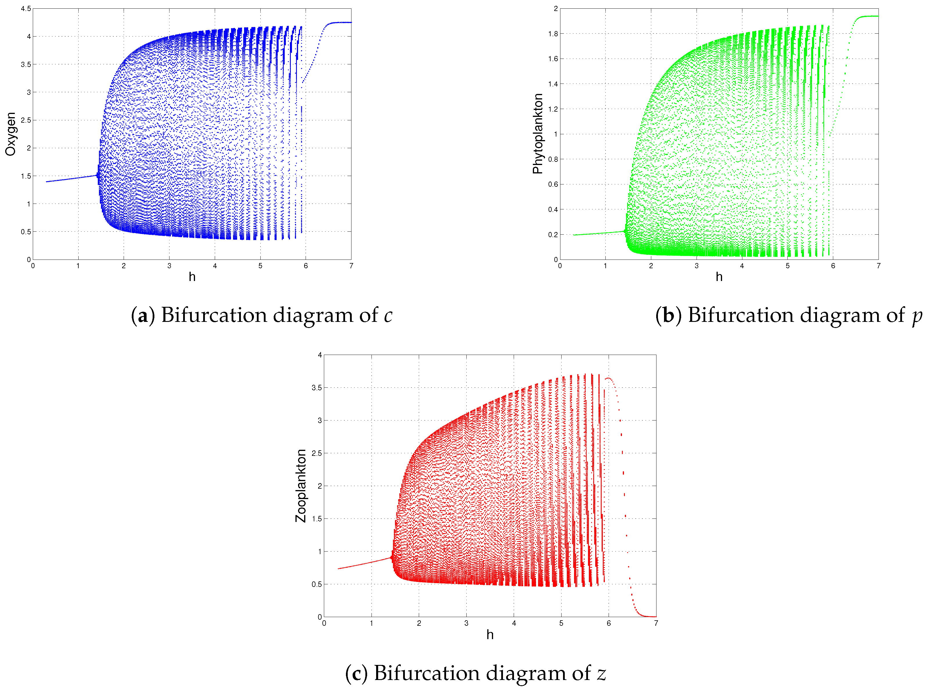
| is stable when and | ||
| h | , and (Figure 12) | is destabilized through Hopf-bifurcation when |
| goes to stable zooplankton free equilibrium when | ||
| is stable when and | ||
| , and (Figure 13) | is destabilized through Hopf-bifurcation when | |
| goes to stable zooplankton free equilibrium when | ||
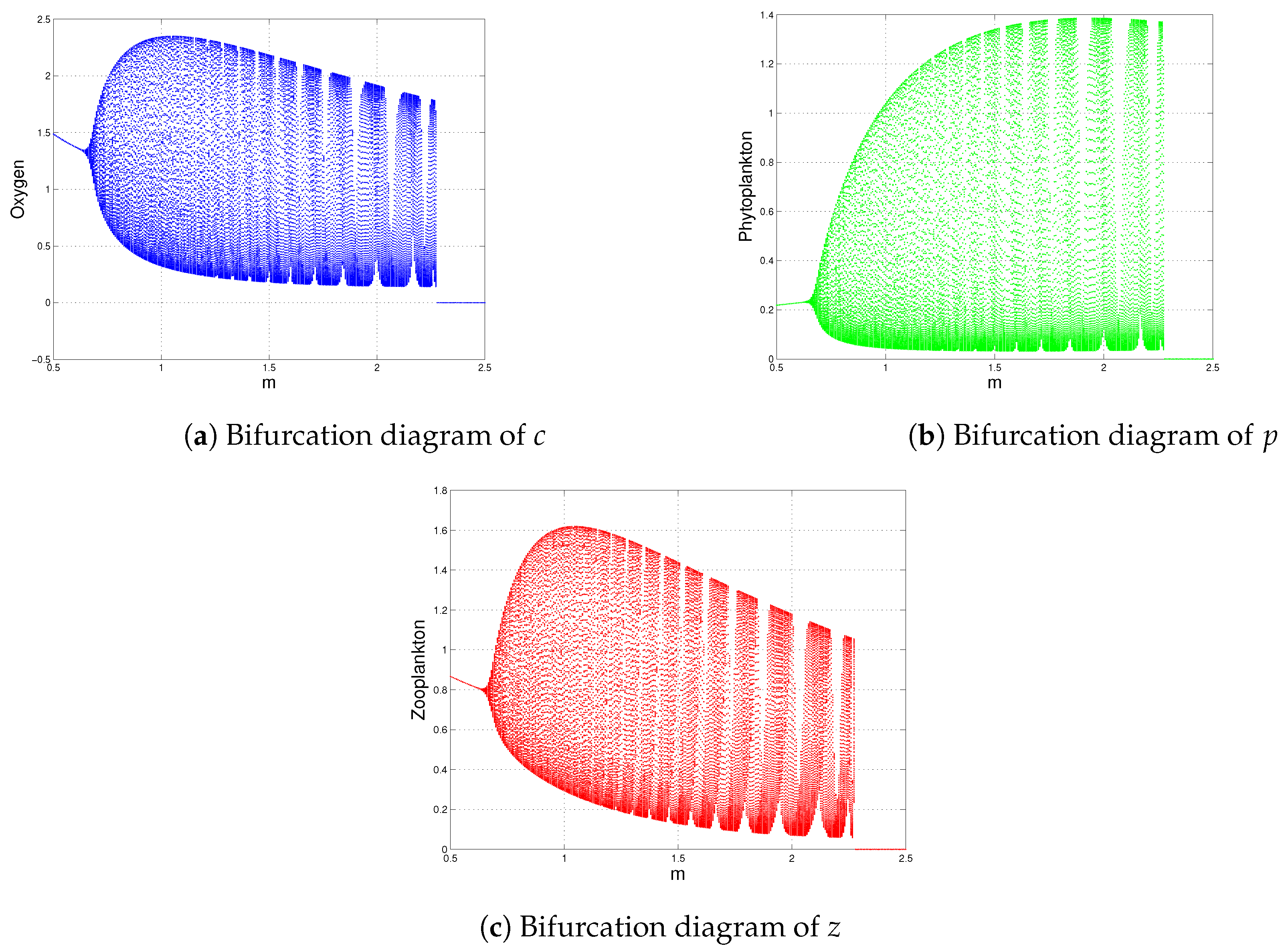
| is stable when | ||
| m | and (Figure 14) | is destabilized through Hopf-bifurcation when |
| goes to when | ||
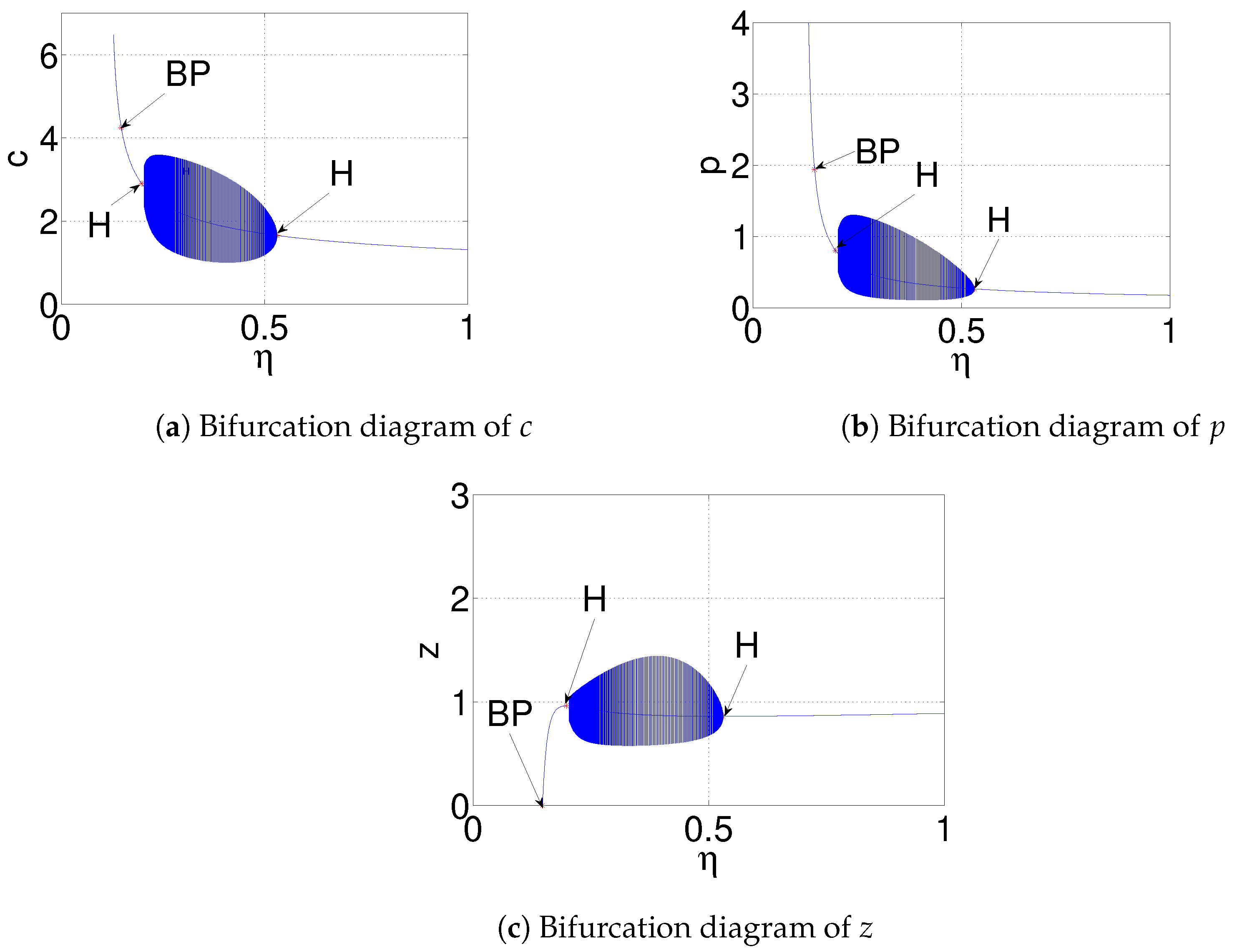
| g | (Figure 15) | is destabilized through Hopf-bifurcation when |
| (if , exists) | ||
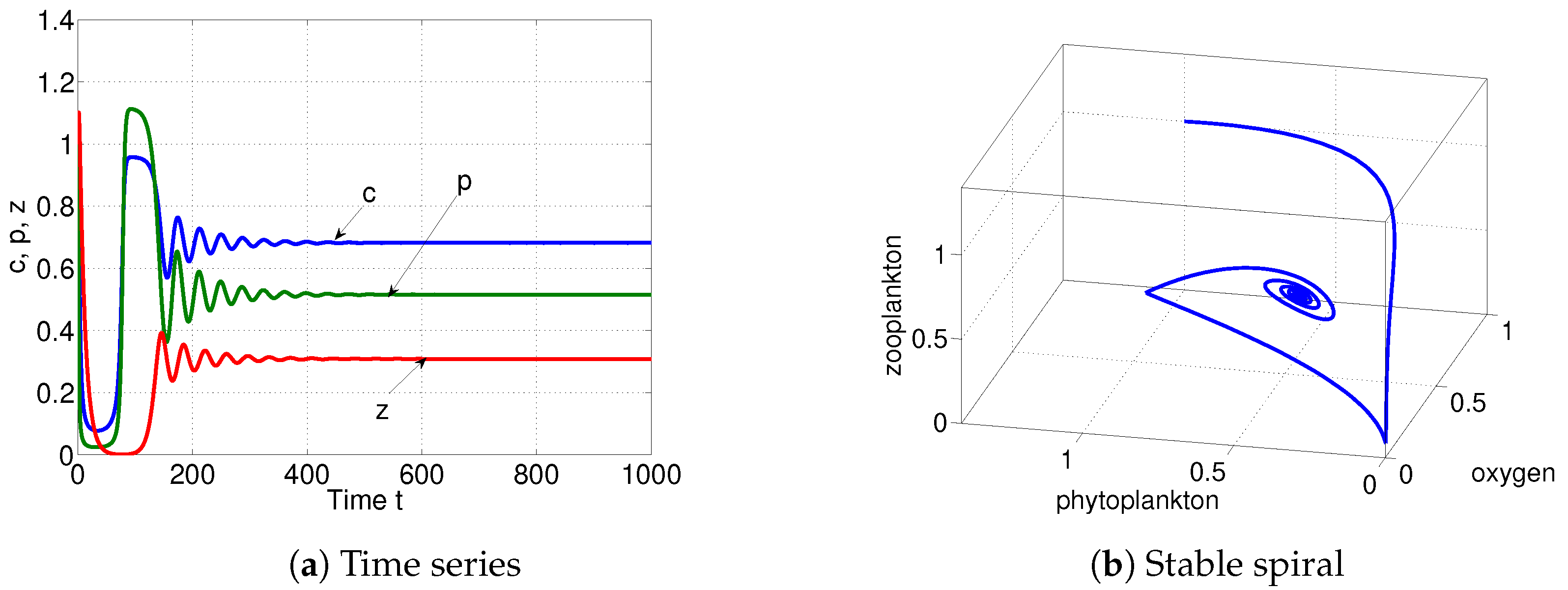
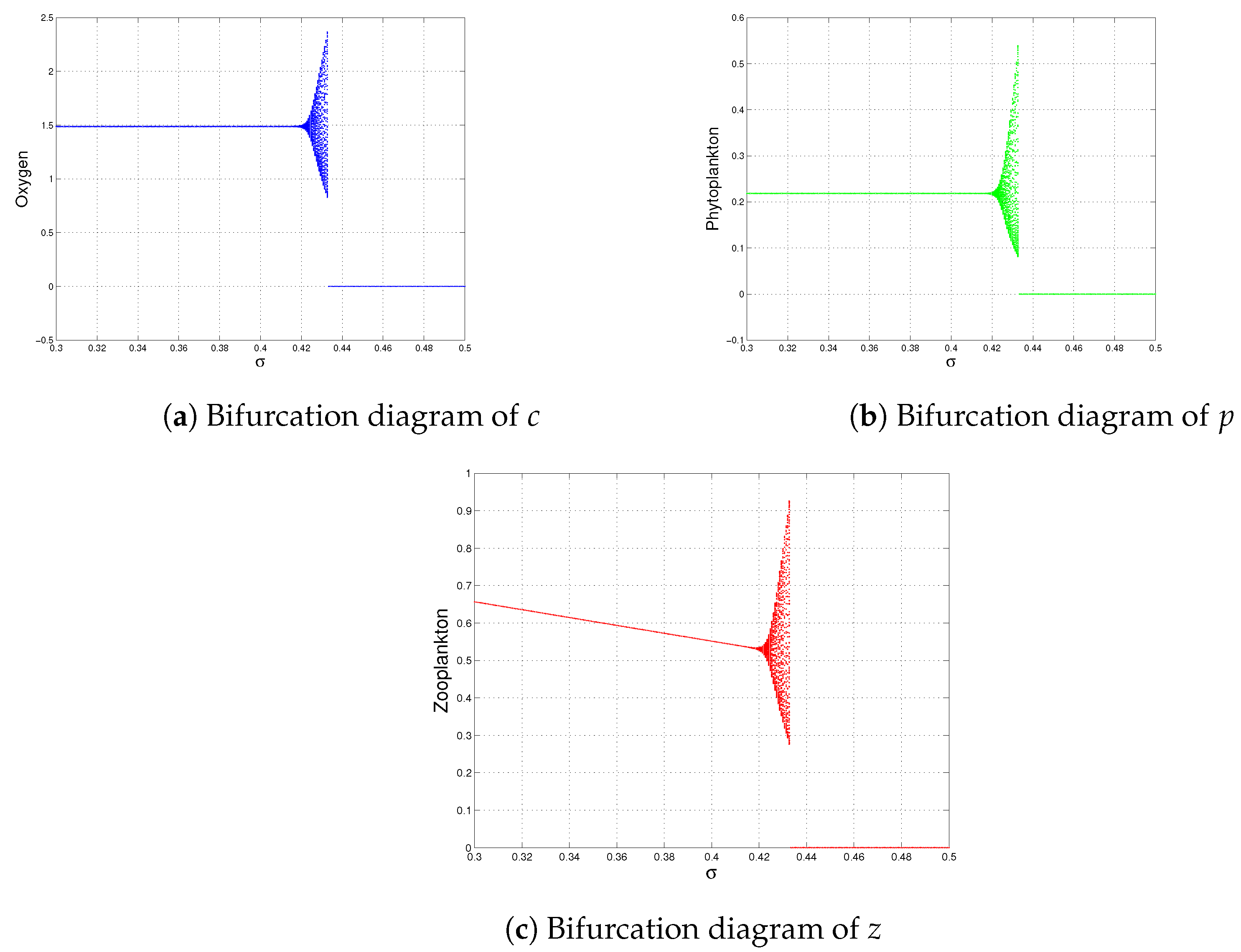
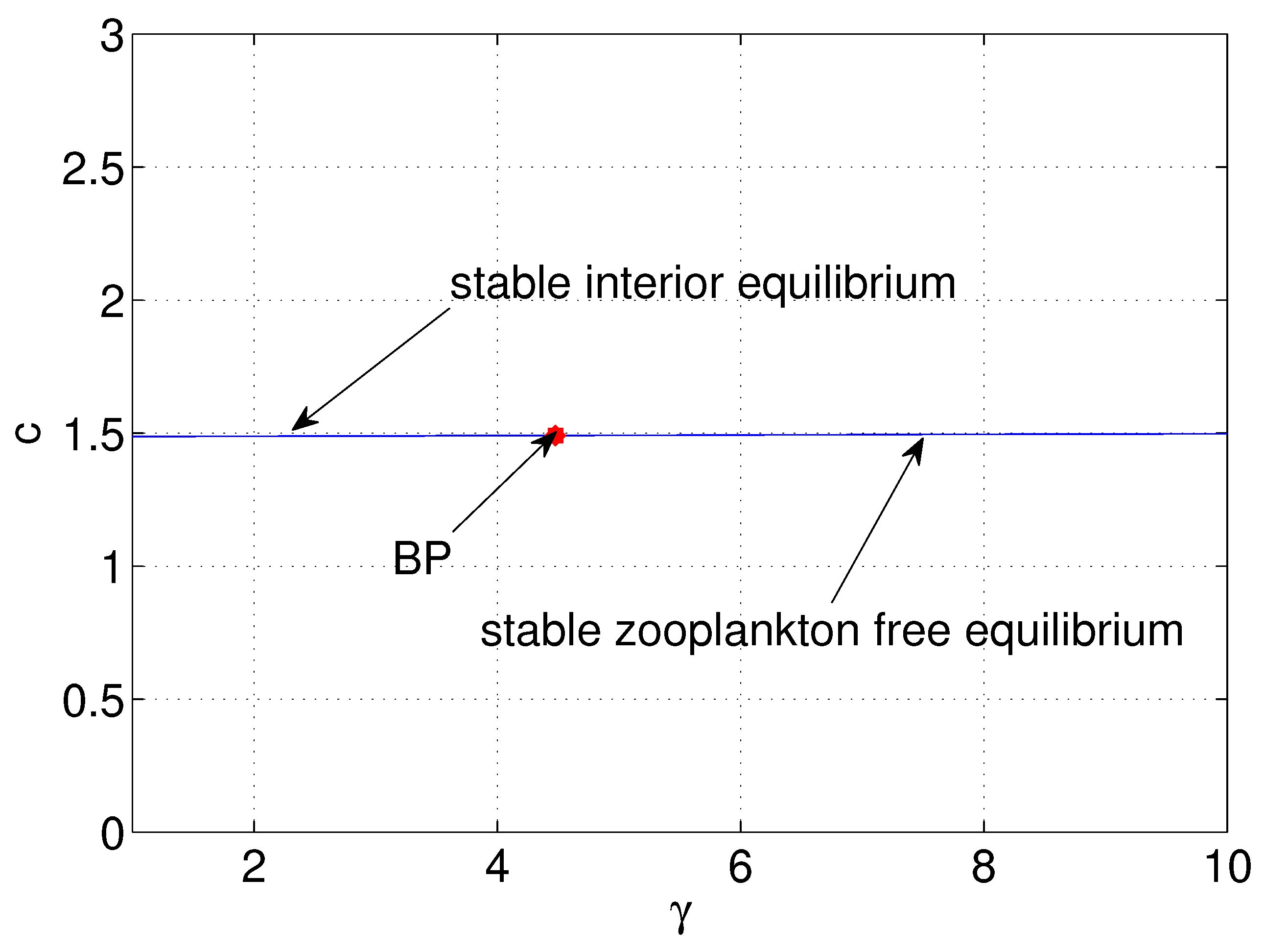
| is stable spiral when | ||
| (zooplankton free equilibrium) is stable when | ||
| , and (Figure 16) | is stable when and | |
| is destabilized through Hopf-bifurcation when | ||
| (zooplankton free equilibrium) is stable when | ||
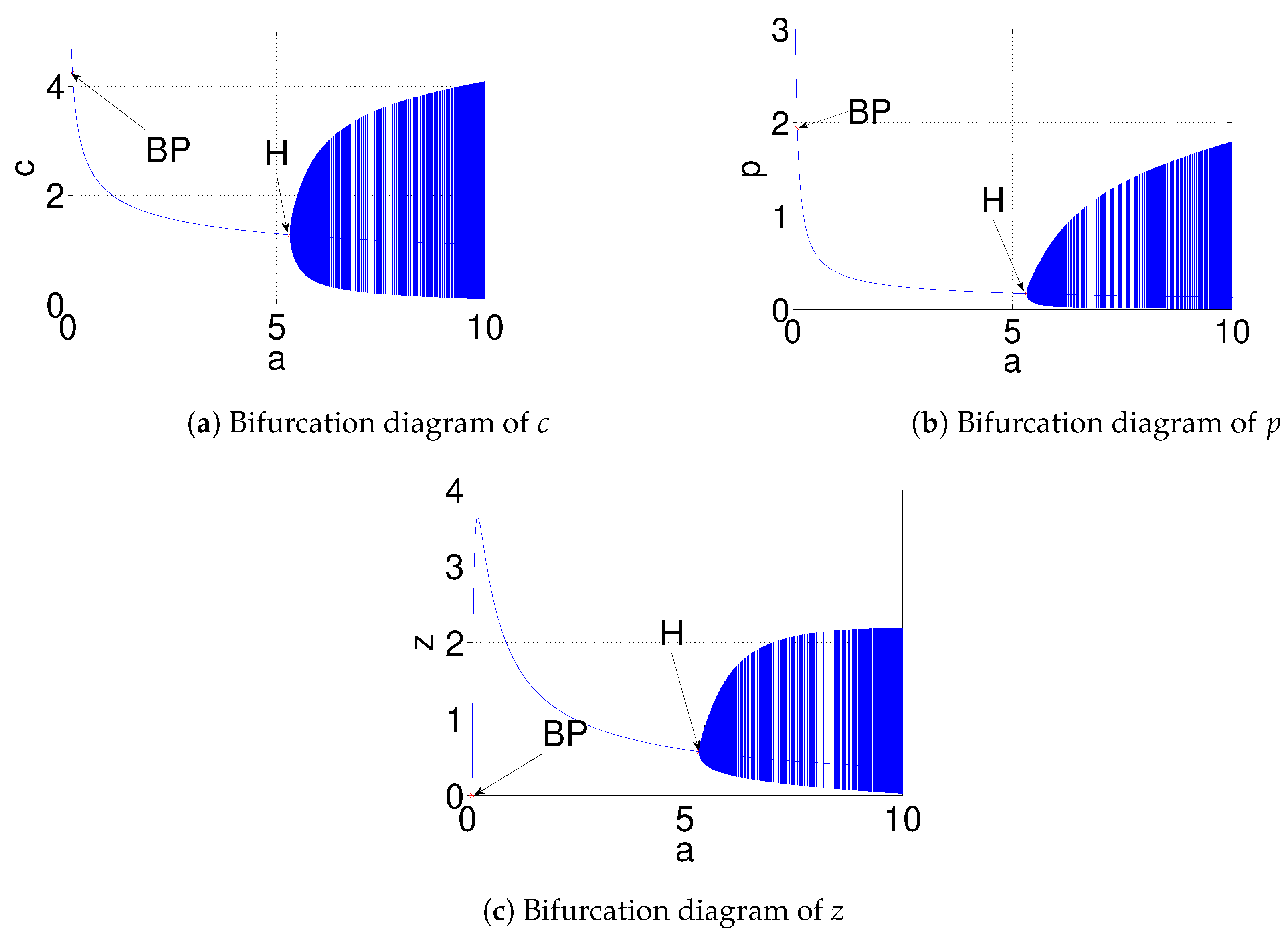
| a | and (Figure 17) | is stable when |
| (Figure 18) | is destabilized through Hopf-bifurcation when | |
| exists and is stable when | ||
| goes to stable zooplankton free equilibrium when |
Publisher’s Note: MDPI stays neutral with regard to jurisdictional claims in published maps and institutional affiliations. |
© 2022 by the authors. Licensee MDPI, Basel, Switzerland. This article is an open access article distributed under the terms and conditions of the Creative Commons Attribution (CC BY) license (https://creativecommons.org/licenses/by/4.0/).
Share and Cite
Mondal, S.; Samanta, G.; De la Sen, M. Dynamics of Oxygen-Plankton Model with Variable Zooplankton Search Rate in Deterministic and Fluctuating Environments. Mathematics 2022, 10, 1641. https://doi.org/10.3390/math10101641
Mondal S, Samanta G, De la Sen M. Dynamics of Oxygen-Plankton Model with Variable Zooplankton Search Rate in Deterministic and Fluctuating Environments. Mathematics. 2022; 10(10):1641. https://doi.org/10.3390/math10101641
Chicago/Turabian StyleMondal, Sudeshna, Guruprasad Samanta, and Manuel De la Sen. 2022. "Dynamics of Oxygen-Plankton Model with Variable Zooplankton Search Rate in Deterministic and Fluctuating Environments" Mathematics 10, no. 10: 1641. https://doi.org/10.3390/math10101641
APA StyleMondal, S., Samanta, G., & De la Sen, M. (2022). Dynamics of Oxygen-Plankton Model with Variable Zooplankton Search Rate in Deterministic and Fluctuating Environments. Mathematics, 10(10), 1641. https://doi.org/10.3390/math10101641