Geometric Metric Learning for Multi-Output Learning

Abstract

Due to its wide applications, multi-output learning that predicts multiple output values for a single input at the same time is becoming more and more attractive. As one of the most popular frameworks for dealing with multi-output learning, the performance of the k-nearest neighbor (kNN) algorithm mainly depends on the metric used to compute the distance between different instances. In this paper, we propose a novel cost-weighted geometric mean metric learning method for multi-output learning. Specifically, this method learns a geometric mean metric which can make the distance between the input embedding and its correct output be smaller than the distance between the input embedding and the outputs of its nearest neighbors. The learned geometric mean metric can discover output dependencies and move the instances with different outputs far away in the embedding space. In addition, our objective function has a closed solution, and thus the calculation speed is very fast. Compared with state-of-the-art methods, it is easier to explain and also has a faster calculation speed. Experiments conducted on two multi-output learning tasks (i.e., multi-label classification and multi-objective regression) have confirmed that our method provides better results than state-of-the-art methods.

1. Introduction

In real-world applications, many machine-learning problems, e.g., multi-label learning and multi-target regression, involving diverse prediction can be classified as multi-output learning. Multi-output learning is an emerging machine-learning paradigm that aims to predict multiple output values of a given input at the same time [1]. For example, text documents or semantic scenes can be assigned to multiple topics; one sensor can output different environmental coefficients; a gene can have multiple biological functions; a patient may suffer from multiple diseases, and so on.

Let there be a multi-output training set $\mathcal{D}=\{{\mathbf{x}}_j,{\mathbf{y}}_j|1\le j\le n\}$, where n is the number of instances, ${\mathbf{x}}_j\in \mathcal{X}$ and ${\mathbf{y}}_j\in \mathcal{Y}$ are the feature vector and the output vector for the j-th instance, respectively, and $\mathcal{X}\in {\mathbb{R}}^p$ denote the p-dimensional input space and $\mathcal{Y}\in {\mathbb{R}}^c$ denote the output space with c output variables. Multi-output learning aims to learn a mapping function $h:\mathcal{X}\to \mathcal{Y}$ from $\mathcal{D}$ to assign an instance with a proper output vector. Compared with the traditional single-output learning, multi-output learning has a multivariate nature and its output values have diverse data types; thus it subsumes many learning problems in many real-world applications. For example, binary output values ${\mathbf{y}}_j\in {\{0,1\}}^c$ can refer to a multi-label classification problem [2] and real-valued outputs ${\mathbf{y}}_j\in {\mathbb{R}}^c$ to a multi-target regression problem [3].

As one of the the most popular frameworks for solving multi-output problems, it has been proven that the k nearest neighbor (kNN) algorithm’s prediction performance can be significantly improved by learning a proper distance metric. For example, by imposing the constraint that two nearby instances from different classes will be pushed further apart with a large margin, Gou et al. [4,5] show that the prediction performance of kNN can be greatly improved. For handling multi-label learing, Zhang et al. [6] proposed a novel maximum margin output coding (MMOC) method based on structural SVMs [7,8]. It learns a distance metric such that the instances with different multiple outputs will be moved far away. Unfortunately, the training and testing of MMOC are time-consuming, which involves both solving a box-constrained quadratic programming (QP) problem for each training sample and a QP problem on ${\{0,1\}}^c$ space, respectively. Even if approximate inference is used to solve this QP problem, it is still computationally expensive. Inspired by kNN and MMOC, Liu et al. [9] proposed a large margin metric learning paradigm (LMMO) for multi-output tasks with only k nearest neighbor constraints, reducing the training computationally complexity from $\mathcal{O}(n{c}^3+np{c}^2+n^4)$ of MMOC to $\mathcal{O}(c^3+knp{c}^2)$ for each iteration, and the testing computationally complexity from $\mathcal{O}\left(c^3\right)$ of MMOC to $\mathcal{O}(cn+pc)$, thus significantly breaking the bottleneck of MMOC. Nevertheless, as the state-of-the-art metric learning method for multi-output learning, the LMMO algorithm adopts the accelerated proximal gradient (APG) method to train LMMO, but cannot directly obtain the optimal metric with a closed-form solution. To achieve an $\epsilon$-solution, the number of iterations needed by APG update is at least $\mathcal{O}\left(\frac{1}{\sqrt{\epsilon }}\right)$. In order to obtain the metric with good performance, more iterations of APG are needed to obtain the more accurate solution.

Therefore, it is non-trivial to develop a gradient-free metric learning algorithm for a multi-output task. To achieve this goal, this paper presents a novel geometric mean metric learning method for multi-output tasks, which learns a cost-weighted metric such that the instances with very different multiple outputs will be moved far away. Our formulation also possesses several attractive properties: closed-form solution, ease of interpretability, and computational speed several orders of magnitude faster than the state-of-the-art method.

Our contributions are as follows. (1) We propose a novel geometric mean metric learning method for multi-output tasks, which possesses several attractive properties: closed-form solution, ease of interpretability, and computational speed several orders of magnitude faster than the state-of-the-art method. (2) Experiments conducted on two multi-output learning tasks have confirmed that our method provides better results than the state-of-the-art methods.

This paper is organized as follows. Section 2 gives related work. Section 3 presents our geometric mean metric learning method for multi-output tasks. The performance of our proposed method for MLC and MTR is evaluated in Section 4. Section 5 concludes the work.

2. Related Work

2.1. Multi-Output Learning

Multi-output learning is an important machine-learning paradigm, which subsumes many learning problems in many practical applications. This paper focuses on the following two most popular multi-output learning tasks, namely multi-label classification and multi-objective regression.

Multi-label Classification aims to predict multiple different labels of a single sample. It has become an attractive emerging field and can be used in many practical applications, such as document classification [10], image retrieval [11], and image annotation [12]. In the past few years, many multi-label classification algorithms have been proposed. According to [2], these methods can be roughly divided into two categories: problem transformation and algorithm adaptation. By transforming popular learning techniques, algorithm adaptation methods try to directly deal with multi-label learning problems. ML-kNN [13], ML-DT [14], and Rank-SVM [15] are the typical methods. By converting the original problem into other well-established learning problems, the problem transformation methods try to use off-the-shelf techniques to solve the problem. Binary relevance [16], random k-labelsets [17], calibrated label ranking [18] and classifier chains [19] are the representive methods.

Multi-target Regression aims to predict the values of multiple continuous target variables for a set of predictor variables. Similar to multi-label learning methods, multi-objective regression methods can also be roughly divided into two categories: algorithm adaptation and problem transformation [20]. Compared with the existing problem transformation methods, the algorithm adaptive methods usually generate a single multi-output model, which is easier to interpret and can be extended to a larger output space. On the other hand, by adopting suitable basic learners, the problem transformation methods can easily adapt to the the problem at hand, and it is found that it is generally better than the algorithm adaptive method in terms of accuracy [21].

2.2. Metric Learning

Given a set of a pair of similar/dissimilar points, metric learning aims to learn the distance metric to keep similar/dissimilar points close/away in the embedding space. The distance metric retains the distance relationship between the training data [22]. The previous works [23,24,25] show that designing appropriate metrics can significantly improve the kNN classification accuracy of single-output learning tasks and multi-output learning tasks.

Metric learning methods can be roughly divided into global distance metric learning and local distance metric learning. Global distance metric learning learns appropriate metrics to keep all data points in the same class close, while pulling instances of different classes away. The most representative methods are found in  [26,27]. The second type of methods tries to learn the distance metric that satisfies the local pairwise constraints, which is particularly useful for the kNN classifier. The most representative methods are found in  [9,28]. However, these methods usually use gradient-based optimization methods to obtain appropriate metrics. On the contrary, we proposed a novel cost-weighted geometric mean metric learning method for multi-output tasks. It learns a cost-weighted metric with a gradient-free optimization method. This makes the learned metric more accurate and the training procedure more efficient.

3. The Proposed Method

3.1. Background

Suppose we are given a multi-output training set with n instances, i.e., $\mathcal{D}=\{{\mathbf{x}}_j,{\mathbf{y}}_j|1\le j\le n\}$, where ${\mathbf{x}}_j\in \mathcal{X}$ and ${\mathbf{y}}_j\in \mathcal{Y}$ are the feature vector and the output vector for the j-th instance, respectively. Multi-output learning aims to learn a function $h:\mathcal{X}\to \mathcal{Y}$ from $\mathcal{D}$ to predict the corresponding output vector of an instance.

To address this problem, a linear regression model simply learns the matrix $\mathbf{W}$ according to the following formulation:

$$\underset{\mathbf{W}\in {\mathbb{R}}^{p\times c}}{min}\frac{1}{2}{\parallel \mathbf{XW}-\mathbf{Y}\parallel }_F^2,$$

(1)

where ${\parallel ·\parallel }_F$ is the Frobenius norm, $\mathbf{X}\in {\mathbb{R}}^{n\times p}$ is the input matrix and $\mathbf{Y}\in {\mathbb{R}}^{n\times c}$ is the output matrix. However, due to a lack of modeling correlations of output space, this method usually yields low performance.

LMMO [9] learns a large margin metric to model correlations of output space. It forces the distance between input ${\mathbf{W}}^T{\mathbf{x}}_i$ and its corresponding output ${\mathbf{y}}_i$ to be smaller than the distance between ${\mathbf{W}}^T{\mathbf{x}}_i$ and the output $\mathbf{y}$ of the nearest neighbors of ${\mathbf{x}}_i$ with at least a margin, which is measured by $\mathsf{\Delta }({\mathbf{y}}_i,\mathbf{y})$, the difference between ${\mathbf{y}}_i$ and $\mathbf{y}$. The large margin metric learning formulation is formulated as follows:

$$\begin{array}{c}\underset{\mathbf{Q}\in S_c^{+},{\left\{{\xi }_i\ge 0\right\}}_{i=1}^n}{min}\frac{1}{2}trace\left(\mathbf{Q}\right)+\frac{C}{n}\sum _{i=1}^n{\xi }_i^2\\ \mathrm{s}.\mathrm{t}.{\varphi }_{{\mathbf{x}}_i,{\mathbf{y}}_i}^T\mathbf{Q}{\varphi }_{{\mathbf{x}}_i,{\mathbf{y}}_i}+\mathsf{\Delta }\left({\mathbf{y}}_i,\mathbf{y}\right)-{\xi }_i\\ \le {\varphi }_{{\mathbf{x}}_i,\mathbf{y}}^T\mathbf{Q}{\varphi }_{{\mathbf{x}}_i,\mathbf{y}},\forall \mathbf{y}\in Nei\left(i\right),\forall i\end{array},$$

(2)

where $S_c^{+}$ represents a $c\times c$ symmetric positive semidefinite matrix, ${\varphi }_{{\mathbf{x}}_i,{\mathbf{y}}_i}={\mathbf{W}}^T{\mathbf{x}}_i-{\mathbf{y}}_i$, ${\xi }_i$ is the slack variable, C is a positive constant that controls the trade-off between the square loss function and the regularizer and $Nei\left(i\right)$ is the output set of k nearest neighbors of input instance ${\mathbf{x}}_i$. The constraints in Equation (2) guarantee that the distance between ${\mathbf{W}}^T{\mathbf{x}}_i$ and its correct output ${\mathbf{y}}_i$ stays closer, but it enlarges the distance between ${\mathbf{W}}^T{\mathbf{x}}_i$ and any other output in the metric space.

However, as the state-of-the-art metric learning method for multi-output learning, the LMMO algorithm cannot directly obtain the optimal metric with a closed-form solution. To achieve an $\epsilon$-solution, the number of iterations needed is at least $\mathcal{O}\left(\frac{1}{\sqrt{\epsilon }}\right)$. Thus, it is worth studying to further improve the computing efficiency of metric learning in multi-output learning.

3.2. Proposed Formulation

It is non-trivial to further obtain a closed-formed solution for LMMO. Inspired by GMML [29], we propose a novel metric learning method with a closed-form solution for multi-output learning, namely, geometric metric learning for cost-weighted multi-output learning (GCMoL), as follows:

$$\underset{\mathbf{Q}\in S_c^{+}}{min}\sum _{i=1}^n\left({\varphi }_{{\mathbf{x}}_i,{\mathbf{y}}_i}^T\mathbf{Q}{\varphi }_{{\mathbf{x}}_i,{\mathbf{y}}_i}+\sum _{\forall \mathbf{y}\in Nei\left(i\right)}\mathsf{\Delta }({\mathbf{y}}_i,\mathbf{y}){\varphi }_{{\mathbf{x}}_i,\mathbf{y}}^T{\mathbf{Q}}^{-1}{\varphi }_{{\mathbf{x}}_i,\mathbf{y}}\right),$$

(3)

where $S_c^{+}$ represents a $c\times c$ symmetric positive semidefinite matrix, ${\varphi }_{{\mathbf{x}}_i,{\mathbf{y}}_i}={\mathbf{W}}^T{\mathbf{x}}_i-{\mathbf{y}}_i$ and $Nei\left(i\right)$ is the output set of k nearest neighbors of input instance ${\mathbf{x}}_i$, and $\mathsf{\Delta }(·)$ represents the cost functions of interest.

Compared with LMMO, in Equation (2), we have transformed several independent inequality constraints into a very uniform formulation. According to Lemma 1, the distance between input ${\mathbf{W}}^T{\mathbf{x}}_i$ and its correct output ${\mathbf{y}}_i$ increases monotonically in $\mathbf{G}$, whereas the distance between ${\mathbf{W}}^T{\mathbf{x}}_i$ and the output $\mathbf{y}$ of the nearest neighbors of ${\mathbf{x}}_i$ decreases monotonically in $\mathbf{G}$. By optimizing the object function in Equation (3), the distance between input ${\mathbf{W}}^T{\mathbf{x}}_i$ and its correct output ${\mathbf{y}}_i$ is naturally smaller than the distance between ${\mathbf{W}}^T{\mathbf{x}}_i$ and the output $\mathbf{y}$ of the nearest neighbors of ${\mathbf{x}}_i$.

For GCMoL, Equation (3), it is cost-weighted of the distance between ${\mathbf{W}}^T{\mathbf{x}}_i$ and the output $\mathbf{y}$ of the nearest neighbors of ${\mathbf{x}}_i$. Thus, by using the loss function $\mathsf{\Delta }(·)$ the metric $\mathbf{G}$ can be learned in the cost-sensitive way. For simplicity, the loss functions $\mathsf{\Delta }(·)={\parallel ·\parallel }_1$ is always used to measure the distance between different outputs for multi-label learning and mutli-target regression.

Lemma 1.

Let $\mathbf{A}$, $\mathbf{B}$ be (strictly) positive definite matrices such that $\mathbf{A}\succ \mathbf{B}$. Then, ${\mathbf{A}}^{-1}\prec {\mathbf{B}}^{-1}$.

In the following, we further simplify the objective function in Equation (3). Let us define the following two matrices:

$$\mathbf{S}:=\sum _{i=1}^n{\varphi }_{{\mathbf{x}}_i,{\mathbf{y}}_i}{\varphi }_{{\mathbf{x}}_i,{\mathbf{y}}_i}^T$$

(4)

$$\mathbf{D}:=\sum _{i=1}^n\sum _{\forall \mathbf{y}\in Nei\left(i\right)}\mathsf{\Delta }({\mathbf{y}}_i,y){\varphi }_{{\mathbf{x}}_i,\mathbf{y}}{\varphi }_{{\mathbf{x}}_i,\mathbf{y}}^T.$$

(5)

Then, the objective function in Equation (3) can be reformulated as

$$\underset{\mathbf{G}}{min}tr\left(\mathbf{GS}\right)+tr\left({\mathbf{G}}^{-1}\mathbf{D}\right).$$

(6)

The minimization problem (6) is both strictly convex and strictly geodesically convex (Theorem 3 of [29]), which is similar to problem (13) of [29]. It has a global optimal solution and a closed form solution as shown below:

$$\mathbf{G}={\mathbf{S}}_{{♯}_{1/2}}^{-1}\mathbf{D}={\mathbf{S}}^{-1/2}{\left({\mathbf{S}}^{1/2}\mathbf{D}{\mathbf{S}}^{1/2}\right)}^{1/2}{\mathbf{S}}^{-1/2}.$$

(7)

Clearly,  solution of (6) is the geometric mean between ${\mathbf{S}}^{-1}$ and $\mathbf{D}$. But the matrix $\mathbf{S}$ might sometimes be non-invertible or near-singular in practice. To address this issue, a regularizing term, which can be used to incorporate prior knowledge about the distance function, is added to the objective function,

$$\underset{\mathbf{G}\succ \mathbf{0}}{min}\lambda D_{\mathrm{sld}}\left(\mathbf{G},{\mathbf{G}}_0\right)+tr\left(\mathbf{G}\mathbf{S}\right)+tr\left({\mathbf{G}}^{-1}\mathbf{D}\right),$$

(8)

where ${\mathbf{G}}_0$ is the “prior” and $D_{\mathrm{sld}}(\mathbf{G},{\mathbf{G}}_0)$ is the symmetrized LogDet divergence, which is equal to

$$D_{\mathrm{sld}}\left(\mathbf{G},{\mathbf{G}}_0\right):=tr\left(\mathbf{G}{\mathbf{G}}_0^{-1}\right)+tr\left({\mathbf{G}}^{-1}{\mathbf{G}}_0\right)-2c.$$

(9)

The minimization problem in (8) also has a closed-form solution,

$${\mathit{G}}_{\mathrm{reg}}={\left(\mathbf{S}+\lambda {\mathbf{G}}_0^{-1}\right)}^{-1}{♯}_{\frac{1}{2}}\left(\mathbf{D}+\lambda {\mathbf{G}}_0\right).$$

(10)

From Equation (10), we can see that the solution is given by the midpoint of the geodesic joining $\mathbf{S}+\lambda {\mathbf{G}}_0^{-1}$ and $\mathbf{D}+\lambda {\mathbf{G}}_0$. From a geodesic viewpoint, assigning different weights to the matrices is also pivotal for the solution of (3). Therefore, we introduce a nonlinear cost guided by Riemannian geometry of the SPD manifold and obtain a weighted version of (3) below:

$$\underset{\mathbf{G}\succ 0}{min}{h}_t\left(\mathbf{G}\right):=(1-t){\delta }_R^2\left(\mathbf{G},{\mathbf{S}}^{-1}\right)+t{\delta }_R^2(\mathbf{G},\mathbf{D}),$$

(11)

where t is a parameter that determines the balance between the cost terms of ${\delta }_R^2\left(\mathbf{G},{\mathbf{S}}^{-1}\right)$ and ${\delta }_R^2(\mathbf{G},\mathbf{D})$. Moreover, ${\delta }_R$ denotes the Riemannian distance

$${\delta }_R(\mathbf{X},\mathbf{Y}):={∥log\left({\mathbf{Y}}^{-1/2}\mathbf{X}{\mathbf{Y}}^{-1/2}\right)∥}_{\mathrm{F}}\mathrm{for}\mathbf{X},\mathbf{Y}\succ 0$$

(12)

on SPD matrices.

The problem outlined in (11) is geodesically covex and its unique solution is the weighted geometric mean

$$\mathbf{G}={\mathbf{S}}^{-1}{♯}_t\mathbf{D}.$$

(13)

Similar to the regularized solution to problem (8), the solution to the regularized form of problem (11) is given by

$${\mathit{G}}_{\mathrm{reg}}={\left(\mathbf{S}+\lambda {\mathbf{G}}_0^{-1}\right)}_{{♯}_t}^{-1}\left(\mathbf{D}+\lambda {\mathbf{G}}_0\right),$$

(14)

for $t\in [0,1]$. In the case where $t=1/2$, it is equal to (10). Many approaches, e.g., Cholesky–Schur and scaled Newton methods, can be used for fast computation of Riemannian geodesics of SPD matrices. In this paper, we use the Cholesky–Schur method to implement the computation of Riemannian geodesics. The summary of our GCMoL algorithm for multi-output learning is presented in Algorithm 1.    

Algorithm 1: GCMoL.

Require: Input: Training dataset matrix $\mathbf{X}\in {\mathbb{R}}^{n\times p}$ and its corresponding output set $\mathbf{Y}\in {\mathbb{R}}^{n\times c}$, the number of nearest neighbors k, the loss    function $\mathsf{\Delta }(·)$, step length of geodesic t, regularization parameter $\lambda$ and prior knowledge ${\mathbf{G}}_0$. Ensure: Output: Regression matrix $\mathbf{W}$ and the learned metric $\mathbf{G}$.   1. Set $\mathbf{W}:=arg{min}_{\mathbf{W}\in {\mathbb{R}}^{p\times c}}\frac{1}{2}{\parallel \mathbf{XW}-\mathbf{Y}\parallel }_F^2$.   2.Search the output set of k nearest neighbors of each input instance,   namely $Nei\left(i\right),\forall i$.   3. Compute $\mathbf{S}={\sum }_{i=1}^n{\varphi }_{{\mathbf{x}}_i,{\mathbf{y}}_i}{\varphi }_{{\mathbf{x}}_i,{\mathbf{y}}_i}^T$.   4. Compute $\mathbf{D}:={\sum }_{i=1}^n{\sum }_{\forall \mathbf{y}\in Nei\left(i\right)}\mathsf{\Delta }({\mathbf{y}}_i,\mathbf{y}){\varphi }_{{\mathbf{x}}_i,\mathbf{y}}{\varphi }_{{\mathbf{x}}_i,\mathbf{y}}^T$.   5. Compute $\mathbf{G}={\left(\mathbf{S}+\lambda {\mathbf{G}}_0^{-1}\right)}_{{♯}_t}^{-1}\left(\mathbf{D}+\lambda {\mathbf{G}}_0\right)$.

3.3. Prediction

In the metric space, our metric learning formulation can make the input ${\mathbf{W}}^T{\mathbf{x}}_i$ and its correct output ${\mathbf{y}}_i$ as close as possible. For a new test instance $\mathbf{x}$, we can obtain its output by a decoding method. In general, the decoding process requires solving the QP problem on a combinatorial space [6], which is computationally expensive. In this paper, we follow the same prediction method as in [9]. Specifically, we find k nearest neighbors for a new testing input instance $\mathbf{x}$ in our learned metric space, where the distance between $\mathbf{x}$ and ${\mathbf{x}}_i$ can be computed as ${({\mathbf{W}}^T\mathbf{x}-{\mathbf{W}}^T{\mathbf{x}}_i)}^T)\mathbf{G}({\mathbf{W}}^T\mathbf{x}-{\mathbf{W}}^T{\mathbf{x}}_i)$. Then, we conduct voting based on weighted nearest neighbors for the prediction. In particular, for multi-label classification problems, we set $0.5$ as the threshold.

3.4. Complexity Analysis

In this subsection, we compare the training and testing time complexity of different methods.

3.4.1. Training Time

The training of MMOC involves an exponential number of constraints and solving a box-constrained QP problem for each training instance. The authors therefore use the over-generating technique with the cutting plane method and CVX (http://cvxr.com/cvx/, accessed on 8 March 2022) to solve these problems, respectively. Because MMOC is optimized based on the gradient method, it is assumed that this method iterates $\eta$ times at least to get the desired performance. From Liu et al. [9], the training time complexity of MMOC is at least $\mathcal{O}(n{c}^3+np{c}^2+n^4)$ for each iteration. Therefore, the total training time complexity of MMOC is at least $\mathcal{O}(\eta n{c}^3+\eta np{c}^2+\eta n^4)$. The training time of LMMO is dominated by the APG algorithm. To achieve an $\epsilon$-solution, the number of iterations needed by the APG update is $\mathcal{O}\left(\frac{1}{\sqrt{\epsilon }}\right)$. According to Liu et al. [30], the time complexity for each iteration is $\mathcal{O}(c^3+knp{c}^2)$. Therefore, the total training time complexity of LMMO is at least $\mathcal{O}(\frac{1}{\sqrt{\epsilon }}{c}^3+\frac{1}{\sqrt{\epsilon }}knp{c}^2)$. The training time of our method (GCMoL) is dominated by the computation of Riemannian geodesics for SPD matrices. Many approaches, e.g., Cholesky–Schur and scaled Newton methods, can be used for fast computation of Riemannian geodesics of SPD matrices. Following [29], we use the Cholesky–Schur method to implement the computation of Riemannian geodesics. So, the time complexity of GCMoL is $\mathcal{O}(c^3+knp{c}^2)$.

3.4.2. Testing Time

We analyze the testing time for each testing instance. Because the test time of MMOC involves solving a QP problem on the ${\{0,1\}}^c$ space, which is essentially a combinatorial optimization problem, it is very intractable. To address this problem, MMOC uses a mean-field approximation to iteratively obtain approximate solutions. The time complexity of each iteration of the average approximate field is $\mathcal{O}\left(c^2\right)$. If it iterates many times until convergence, its time complexity is at least $\mathcal{O}\left(c^3\right)$. Both LMMO and our method (GCMoL) use the same prediction method and therefore have the same prediction time complexity, i.e., $\mathcal{O}(nc+pc)$.

4. Experiments

In this section, we extensively compared the proposed GCMoL method with related approaches on real-world multi-label classification and multi-target regression datasets. All the methods compared are implemented in MatLab. All experiments are conducted on a desktop with a 3.2 GHZ Intel CPU and 32 GB main memory running on a Windows platform.

4.1. Experimental Setup

(1) Datasets: We conduct experiments on five benchmark multi-label datasets (http://mulan.sourceforge.net/, accessed on 9 March 2022), including emotions, scene, cal500 and genbase, and four benchmark multi-target regression datasets (http://mulan.sourceforge.net/, accessed on 9 March 2022), including edm, enb, jura, and scpf. We summarize the dataset details in the

Table 1. Characteristics of datasets.

$\mathbf{Cat}\left(\mathit{S}\right)$	Dataset	$\left|\mathit{S}\right|$	$\mathit{dim}\left(\mathit{S}\right)$	$\mathit{L}\left(\mathit{S}\right)$	$\mathbf{Card}\left(\mathit{S}\right)$
MLC	emotions	593	72	6	1.869
	scene	2407	294	6	1.074
	cal500	502	68	174	26.044
	genbase	662	1186	27	1.252
MTR	edm	154	16	2	-
	enb	768	8	2	-
	jura	359	15	3	-
	scpf	1137	23	3	-

, where $\left|S\right|$ represents the number of examples, $dim\left(S\right)$ represents the number of features, $L\left(S\right)$ represents the number of class labels, and $Card\left(S\right)$ represents the average number of labels per example, $Dom\left(S\right)$ represents the feature type of the dataset S, and $Cat$ represents the type of task category.

(2) Evaluation Metrics: To testify to the performance, we focus on two evaluation metrics, i.e., Micro-F1 and Macro-F1, for multi-label classification datasets, and one evaluation metric, i.e., aRMAE, for multi-target regression datasets. For Micro-F1 and Macro-F1, the larger the values the better the performance. Their concrete metric definitions are defined in [2]. For aRMAE, the smaller the values the better the performance. It is defined as:

$$aRMAE(\mathbf{h},\mathbf{D})=\frac{1}{m}\sum _{j=1}^m\frac{{\sum }_{(\mathbf{x},\mathbf{y})\in D}\left|{\widehat{y}}_j-y_j\right|}{{\sum }_{(\mathbf{x},\mathbf{y})\in D}\left|{\overline{Y}}_j-y_j\right|},$$

(15)

where ${\overline{Y}}_j$ is the mean value of $Y_j$ over dataset $\mathbf{D}$ and ${\widehat{y}}_j$ is the prediction of $\mathbf{h}$ for $Y_j$. Intuitively, aRMAE measures how much better ($aRMAE<1$) or worse ($aRMAE>1$) the prediction model is compared to a naive baseline that always predicts the mean value of each target.

(3) Comparing Methods: We compare our proposed method GCMoL with the following state-of-the-art multi-output learning methods.

• BR [16] is the most intuitive solution to multi-label learning. It works by decomposing the multi-label learning task into multiple independent binary learning tasks, so it is a problem transformation method. In order to be fair in the experiment, we use the kNN model as the base classifier and set $k=10$.
• ML-kNN [13] is also a problem transformation method, which learns a classifier for each label by combining kNN and Bayesian inference. According to [13], we still use $k=10$ in our experiments, which usually yields the best performance.
• LMMO [9] is a recently proposed large-margin metric learning method for multi-output tasks. It projects both input and output into the same embedding space, and then learns a distance metric to keep instances with the same output close and instances with very different outputs farther away. Its formulation is presented in Equation (2) and can only be used for multi-label learning task. Parameter $\lambda$ is selected from $\{{10}^{-5},{10}^{-4},\dots ,{10}^4,{10}^5\}$.

The hyper-parameters in compared methods are selected via 10-fold cross-validation on the training set. The parameter $\lambda$ is selected from $\{{10}^{-5},{10}^{-4},\dots ,{10}^4,{10}^5\}$, and t is selected from $\{0.2,0.5,0.7\}$. We adopt $k=10$, which yields the best performance.

4.2. Experimental Results

Detailed experimental results are reported in

Table 2. Experimental results for multi-output learning. The best ones are in bold.

Task	Criteria	Dataset	Method
			BR	MLkNN	LMMO	GCMoL
MLC	Micro-F1	emotions	0.4905	0.4918	0.6753	0.6774
		genbase	0.9607	0.9505	0.9697	0.9791
		yeast	0.6330	0.6392	0.5600	0.6376
		CAL500	0.3131	0.3185	0.3339	0.3709
	Macro-F1	emotions	0.4170	0.3811	0.6563	0.6634
		genbase	0.5683	0.5321	0.5877	0.6258
		yeast	0.3892	0.3697	0.3748	0.4056
		CAL500	0.0738	0.0534	0.0689	0.1049
MTR	aRMAE	edm	0.9335	-	0.9010	0.8591
		enb	0.2230	-	0.2488	0.1538
		jura	0.6030	-	0.7158	0.5704
		wq	0.8628	-	0.9933	0.8713

, where the performance rank on each dataset is also shown in the parentheses. Moreover, to show whether GCMoL achieves statistically superior performance against compared approaches, we employ a Nemenyi test (at $0.05$ significance level) whose statistical test results are summarized in Figure 1. The performances between two methods will be significantly different if their average ranks differ by at least one critical difference $CD=q_{\alpha }\sqrt{k(k+1)/6N}$. For the Nemenyi test, $q_{\alpha }=$ at significance level $\alpha =0.05$, and thus $CD=1.2075(k=4,N=12)$. In Figure 1, the connected algorithms indicate that their average rank difference is within one CD. Any unconnected pair of algorithms is considered to have a significant difference in performance.

Based on the reported experimental results, the following observations can be made: (1) Regarding Micro-F1 of the MLC task, GCMoL is basically better than other methods and only slightly inferior to MLkNN on the yeast dataset. (2) Regrading Macro-F1 of the MLC task, GCMoL is always better than other methods. (3) Regarding aRMAE of the MTR task, GCMoL is also basically better than other methods and only slightly inferior to BR on the wq dataset. (4) According to the Nemenyi test results, MLKNN, LMMO, and BR perform not significantly differently from each other, but GCMoL performs significantly better than other methods, which verifies the effectiveness of our method.

4.3. Analysis

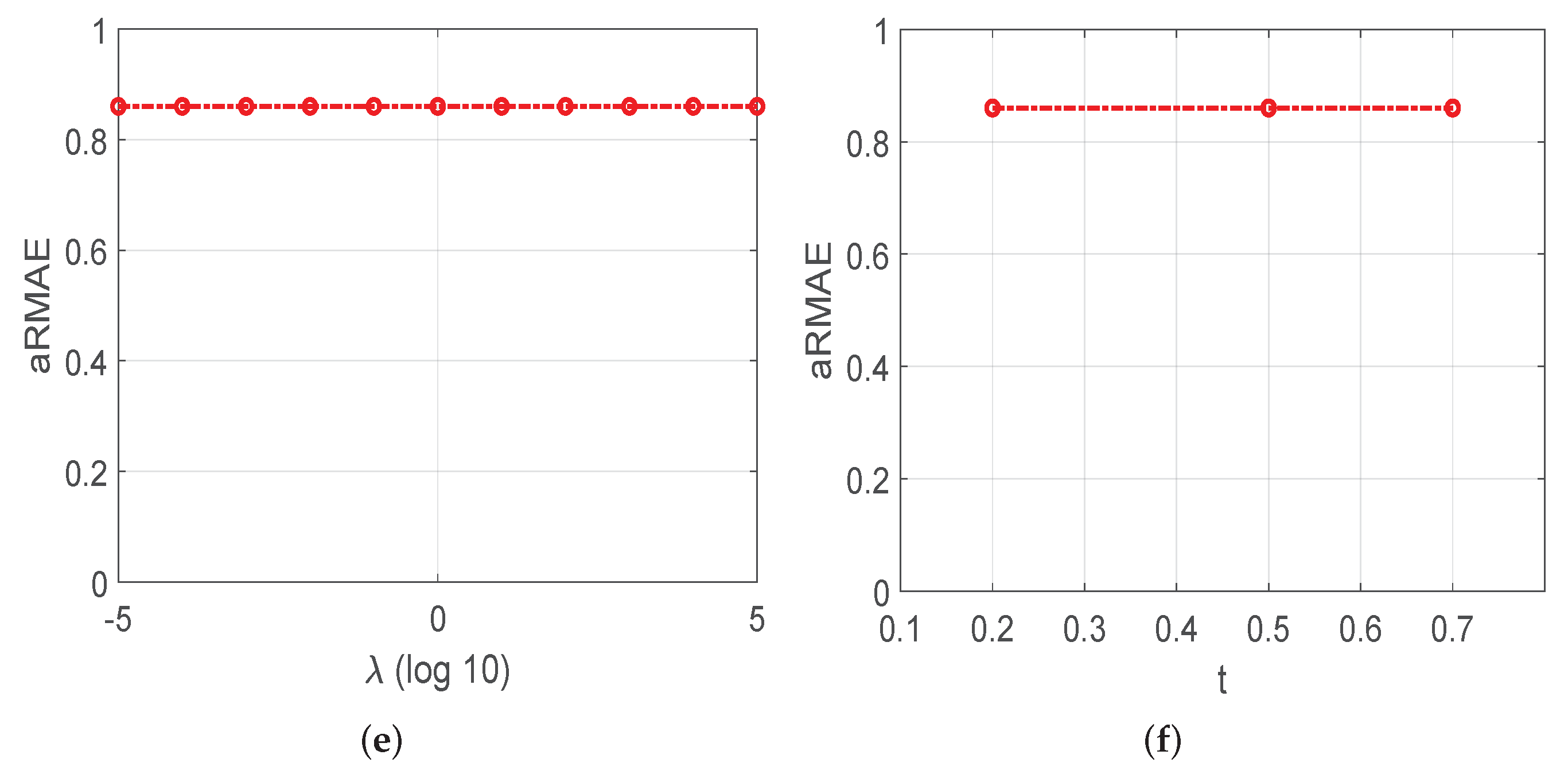
4.3.1. Hyper-Parameter Sensitivity Analysis

There are two hyper-parameters, i.e., $\lambda$ and t, in our proposed method. To give their sensitivity analysis, we conduct experiments on CAL500 and edm datasets. The experimental results of GCMoL with different values of $\lambda$ and t are depicted in Figure 2a–f. From the experimental results, we note that the performance of GCMoL is relatively insensitive to the value of $\lambda$ and t.

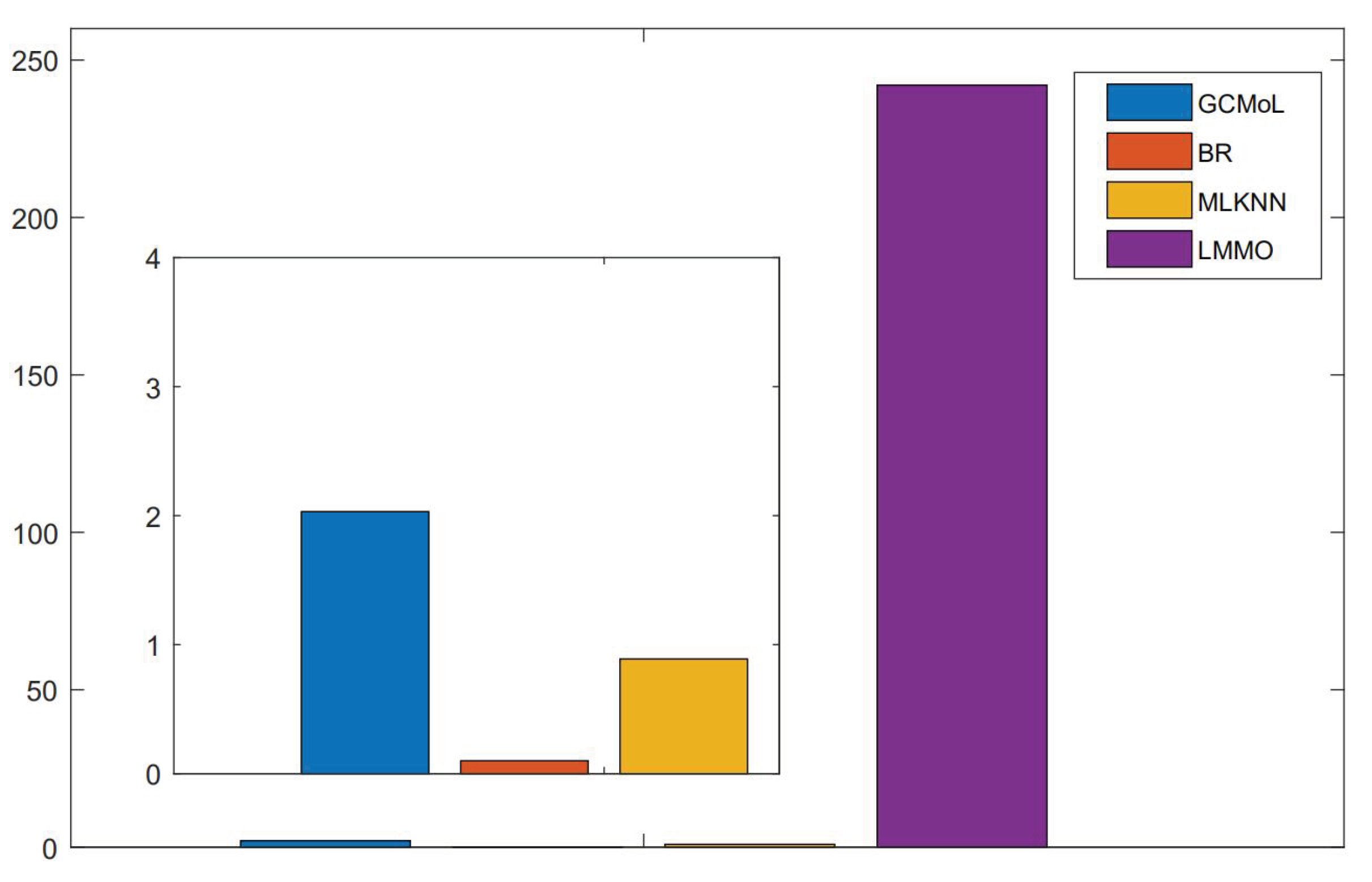
4.3.2. Time-Comsuming Analysis

To further compare the time consumption of different methods, Figure 3 reports the single training time of 10-fold cross validation of our method and baseline approaches in terms of CAL500 dataset. The results illustrate that BR, MLkNN, and GCMoL complete the training in 3 s, but LMMO lasts more than 240 s. Our method is almost 100 times faster than LMMO. In Section 3.4, the results of theoretical analysis for the time complexity show that our method runs slower than BR and MLkNN, but faster than LMMO. The experimental results also confirmed this conclusion.

5. Conclusions

We proposed a novel cost-weighted geometric mean metric learning method for multi-output tasks in this paper. Our method can model output dependency by the learned geometric mean metric, which can make the instances with very different outputs far away. It also admits a closed-form solution and computational speed several orders of magnitude faster than the state-of-the-art LMMO method. Experiments show that our method outperforms the state-of-the-art methods on multi-output learning tasks.

There are several directions worth exploring further in our future work. First, we will try to design a novel robust geometric metric learning method to generalize our technique to weakly supervised multi-output learning task. In weakly supervised multi-output learning tasks, missing or noisy supervision information may bring great challenges to metric learning. Secondly, we will try to design new weakly supervised contrastive learning methods to effectively apply self-supervised learning techniques to a multi-output learning task.

References

1. Xu, D.; Shi, Y.; Tsang, I.W.; Ong, Y.S.; Gong, C.; Shen, X. Survey on Multi-Output Learning. IEEE Trans. Neural Netw. Learn. Syst. 2019, 31, 2409–2429. [Google Scholar] [CrossRef] [Green Version]
2. Zhang, M.L.; Zhou, Z.H. A review on multi-label learning algorithms. IEEE Trans. Knowl. Data Eng. 2013, 26, 1819–1837. [Google Scholar] [CrossRef]
3. Borchani, H.; Varando, G.; Bielza, C.; Larrañaga, P. A survey on multi-output regression. Wiley Interdiscip. Rev. Data Min. Knowl. Discov. 2015, 5, 216–233. [Google Scholar] [CrossRef] [Green Version]
4. Gou, J.; Qiu, W.; Yi, Z.; Shen, X.; Zhan, Y.; Ou, W. Locality constrained representation-based K-nearest neighbor classification. Knowl.-Based Syst. 2019, 167, 38–52. [Google Scholar] [CrossRef]
5. Gou, J.; Sun, L.; Du, L.; Ma, H.; Xiong, T.; Ou, W.; Zhan, Y. A representation coefficient-based k-nearest centroid neighbor classifier. Expert Syst. Appl. 2022, 194, 116529. [Google Scholar] [CrossRef]
6. Zhang, Y.; Schneider, J. Maximum margin output coding. In Proceedings of the 29th International Coference on International Conference on Machine Learning, Edinburgh, UK, 26 June–1 July 2012; pp. 379–386. [Google Scholar]
7. Tsochantaridis, I.; Joachims, T.; Hofmann, T.; Altun, Y. Large margin methods for structured and interdependent output variables. J. Mach. Learn. Res. 2005, 6, 1453–1484. [Google Scholar]
8. BakIr, G.; Hofmann, T.; Schölkopf, B.; Smola, A.J.; Taskar, B.; Vishwanathan, S. Generalization Bounds and Consistency for Structured Labeling; MIT Press: Cambridge, MA, USA, 2007. [Google Scholar]
9. Liu, W.; Xu, D.; Tsang, I.W.; Zhang, W. Metric learning for multi-output tasks. IEEE Trans. Pattern Anal. Mach. Intell. 2018, 41, 408–422. [Google Scholar] [CrossRef] [PubMed]
10. Rubin, T.N.; Chambers, A.; Smyth, P.; Steyvers, M. Statistical topic models for multi-label document classification. Mach. Learn. 2012, 88, 157–208. [Google Scholar] [CrossRef] [Green Version]
11. Verma, Y.; Jawahar, C. Image annotation by propagating labels from semantic neighbourhoods. Int. J. Comput. Vis. 2017, 121, 126–148. [Google Scholar] [CrossRef]
12. Nguyen, C.T.; Zhan, D.C.; Zhou, Z.H. Multi-modal image annotation with multi-instance multi-label LDA. In Proceedings of the Twenty-Third International Joint Conference on Artificial Intelligence, Beijing, China, 3–9 August 2013. [Google Scholar]
13. Zhang, M.L.; Zhou, Z.H. ML-KNN: A lazy learning approach to multi-label learning. Pattern Recognit. 2007, 40, 2038–2048. [Google Scholar] [CrossRef] [Green Version]
14. Clare, A.; King, R.D. Knowledge discovery in multi-label phenotype data. In Proceedings of the European Conference on Principles of Data Mining and Knowledge Discovery, Freiburg, Germany, 3–5 September 2001; Springer: Berlin/Heidelberg, Germany, 2001; pp. 42–53. [Google Scholar]
15. Elisseeff, A.; Weston, J. A kernel method for multi-labelled classification. In Advances in Neural Information Processing Systems; Springer: Berlin/Heidelberg, Germany, 2002; pp. 681–687. [Google Scholar]
16. Boutell, M.R.; Luo, J.; Shen, X.; Brown, C.M. Learning multi-label scene classification. Pattern Recognit. 2004, 37, 1757–1771. [Google Scholar] [CrossRef] [Green Version]
17. Tsoumakas, G.; Vlahavas, I. Random k-labelsets: An ensemble method for multilabel classification. In Proceedings of the European Conference on Machine Learning, Warsaw, Poland, 17–21 September 2007; Springer: Berlin/Heidelberg, Germany, 2007; pp. 406–417. [Google Scholar]
18. Fürnkranz, J.; Hüllermeier, E.; Mencía, E.L.; Brinker, K. Multilabel classification via calibrated label ranking. Mach. Learn. 2008, 73, 133–153. [Google Scholar] [CrossRef] [Green Version]
19. Read, J.; Pfahringer, B.; Holmes, G.; Frank, E. Classifier chains for multi-label classification. Mach. Learn. 2011, 85, 333. [Google Scholar] [CrossRef] [Green Version]
20. Spyromitros-Xioufis, E.; Sechidis, K.; Vlahavas, I. Multi-target regression via output space quantization. arXiv 2020, arXiv:2003.09896. [Google Scholar]
21. Spyromitros-Xioufis, E.; Tsoumakas, G.; Groves, W.; Vlahavas, I. Multi-target regression via input space expansion: Treating targets as inputs. Mach. Learn. 2016, 104, 55–98. [Google Scholar] [CrossRef] [Green Version]
22. Yang, L.; Jin, R. Distance metric learning: A comprehensive survey. Mich. State Univ. 2006, 2, 4. [Google Scholar]
23. He, X.; King, O.; Ma, W.Y.; Li, M.; Zhang, H.J. Learning a semantic space from user’s relevance feedback for image retrieval. IEEE Trans. Circuits Syst. Video Technol. 2003, 13, 39–48. [Google Scholar]
24. He, X.; Ma, W.Y.; Zhang, H.J. Learning an image manifold for retrieval. In Proceedings of the 12th Annual ACM International Conference on Multimedia, New York, NY, USA, 10–16 October 2004; pp. 17–23. [Google Scholar]
25. He, J.; Li, M.; Zhang, H.J.; Tong, H.; Zhang, C. Manifold-ranking based image retrieval. In Proceedings of the 12th Annual ACM International Conference on Multimedia, New York, NY, USA, 10–16 October 2004; pp. 9–16. [Google Scholar]
26. Weinberger, K.Q.; Saul, L.K. Distance metric learning for large margin nearest neighbor classification. J. Mach. Learn. Res. 2009, 10, 207–244. [Google Scholar]
27. Xing, E.P.; Jordan, M.I.; Russell, S.J.; Ng, A.Y. Distance metric learning with application to clustering with side-information. In Advances in Neural Information Processing Systems; Springer: Berlin/Heidelberg, Germany, 2003; pp. 521–528. [Google Scholar]
28. Peng, J.; Heisterkamp, D.R.; Dai, H. Adaptive kernel metric nearest neighbor classification. In Proceedings of the 2002 International Conference on Pattern Recognition, Quebec City, QC, Canada, 11–15 August 2002; Volume 3, pp. 33–36. [Google Scholar]
29. Zadeh, P.; Hosseini, R.; Sra, S. Geometric mean metric learning. In Proceedings of the International Conference on Machine Learning, New York, NY, USA, 19–24 June 2016; pp. 2464–2471. [Google Scholar]
30. Liu, W.; Tsang, I.W. Large margin metric learning for multi-label prediction. In Proceedings of the Twenty-Ninth AAAI Conference on Artificial Intelligence, Austin, TX, USA, 25–30 January 2015. [Google Scholar]
Figure 1. Comparison of GCMoL against other comparing algorithms with the Nemenyi test.
Mathematics 10 01632 g001
Figure 2. Sensitivity analysis about GCMoL with different λ and t. (a) Micro-F1 scores of different λ on CAL500 dataset. (b) Micro-F1 scores of different t on CAL500 dataset. (c) Macro-F1 scores of different λ on CAL500 dataset. (d) Macro-F1 scores of different t on CAL500 dataset. (e) aRMAE of different λ on edm dataset. (f) aRMAE of different t on edm dataset.
Mathematics 10 01632 g002aMathematics 10 01632 g002b
Figure 3. Running time results of different methods on the CAL500 dataset.
Mathematics 10 01632 g003