1. Introduction
Currently, in connection with new requirements for the properties of structural materials, for the conditions of their operation, as well as in connection with the development of new technologies, which are characterized by high gradients of temperature and deformation fields, the attention to the related problems of the mechanics of deformable bodies requires revision, since the associated effects can be significant, although, in the traditional approach, they are usually ignored, i.e., changes in elastic deformation in the case of classical unbound thermoelasticity do not affect the temperature distribution, and vice versa.
One of the first attempts to eliminate this shortcoming of the classical uncoupled theory when describing the dynamic behavior of structures can be found in [
1]. However, in the formulated theory of coupled thermoelasticity in [
1], diffusion-type heat transfer models were used, predicting infinite heat propagation rates, which contradicts experimental observations. Subsequently, these contradictions were removed as a result of the development of a generalization of the theory of heat conduction [
2,
3,
4]. The idea of studying connected processes of thermodynamics of deformations and thermal conductivity problems led to the development of a generalized model of hyperbolic thermal conductivity in [
5,
6,
7,
8].
The physical nature of the relaxation time in the Maxwell–Cattaneo heat conduction law was discussed in [
9], where it was proposed to associate the relaxation time with the viscoelastic properties of the media.
Further development of the study of coupled thermoelasticity and thermal conductivity on the basis of the generalized theory of thermal conductivity was obtained in works [
10,
11] and others.
The importance of taking into account temperature gradient effects of a higher order in comparison with classical models was noted in [
12,
13,
14]. First of all, we should celebrate the fundamental work of [
15], where a unified procedure for constructing coupled gradient models of thermodynamic processes of deformation for gradient and nonlocal materials (constitutive relations, equations of motion, and initial boundary conditions) is consistently presented using the thermodynamic restrictions extended to the cases of gradient media. Taking into account the coupled effects of the deformation fields and temperatures is traditionally of considerable interest for the applications. As an example, let us consider the work [
16], in which a coupled thermoelasticity mode was used to study the effect of temperature relaxation on transient processes at the top of a semi-infinite crack. A special Fourier model with one and two relaxation times was used for modeling. To describe coupled processes of thermomechanics in inhomogeneous structures, a version of the generalized gradient model with two scale parameters was formulated in [
17].
In recent work [
18], a coupled gradient thermoelasticity model and a dual-phase-lag heat conduction model were used to study the processes of thermoelastic damping in strain gradient microplates. Simular model is applied in [
19] to study the thermal heat problem of a homogeneous and isotropic long cylinder due to initial stress and heat source. The possible elastic flexural waves in a thermoelastic semiconduction micro-beam are studied in the work [
20]. The coupling effects of the carrier field, temperature field, and the elastic displacement field are considered. The strain gradient elasticity and the non-Fourier the dual-phase-lag heat conduction model were incorporated into a generalized thermoelastic model to take the small-scale effects into account for the thermoelastic damping in microplates.
As a rule, the effects of coupling are limited by taking into account the coupling of temperature fields with volumetric deformation and the corresponding dynamic effects determined by the generalized laws of heat conduction [
16,
17,
18,
19,
20,
21], etc. In this connection, the novelty of the present work lies in the fact that it attempts to take into account the effects of higher order coupling between the gradients of the temperature fields and the gradients of the deformation fields.
For inhomogeneous structures, when solving related problems, it is important to take into account surface effects at the interface between different phases—the effects of thermal resistance of the boundaries [
22,
23,
24]. In this regard, in the work [
25], it is shown that the use of the gradient model of stationary thermal conductivity together with an extended version of continuous adhesion makes it possible to model successfully the thermal resistance.
A new and fairly general coupled model of thermoelasticity and thermal conductivity was proposed in [
25,
26], where a variational gradient model of a medium with a field of defects—dilatation—was proposed. The model took into account the mutual influence of elastic strain fields and defect fields determined by free dilatation. In turn, the defect fields—free dilatations—are proposed to be interpreted as temperature deformations.
As a result, a coupled gradient two-parameter model of thermoelasticity and thermal conductivity was constructed, in which scale effects are determined, both in mechanical processes and in processes of stationary thermal conductivity, and the coupleness of these processes is determined by the coupleness of elastic deformation fields and temperature deformation fields in the version of the gradient generalization of the Mindlin model for dilatation model of defects. It is shown that the model is fully consistent with thermoelasticity and thermal conductivity, since, in particular, it describes both the gradient version of thermoelasticity and gradient thermal conductivity.
In a recent paper [
27], a generalization of the variational model considered earlier in [
25,
26] was proposed, in which a more complete gradient one-parameter model of the interphase layer (not only the dilatation gradient model) for a medium with a defect field, the free dilatation field, is used to describe mechanical processes (field of thermal deformations), and also a non-classical version of the model of adhesive interactions is introduced, which allows modeling of thermal resistance. The study of the structures of general solutions for the proposed connected model and the features of the fundamental solutions obtained for this problem are analytically given in [
27].
In this work, the general solution of the coupled stationary problem of thermoelasticity and thermal conductivity is constructed in the form of an expansion in fundamental solutions characteristic of a coupled formulation, taking into account the constraints on the model parameters associated with positive definiteness. Such representations are new and are used for the first time for a qualitative analysis of possible solutions to contact problems. In particular, we will study the structure of the general solution and the features of the deformed state and thermal fields depending on the coupled parameters, scale parameters, and the parameter responsible for thermal barrier effects.
Let us consider the variational statement of the coupled problem [
27], where the gradient model of the interphase layer is introduced for a medium with defect fields (thermal strains) and a model of surface interactions is taken into account [
25]:
where
,
and
are the Lamé elastic parameters,
,
are the scale parameters that define the gradient effect for the temperature and elastic gradient effect consequently,
is the thermal conductivity coefficient,
determines the coefficient of thermal expansion,
defines the coupled thermomechanical effects,
defines the thermal resistance effects on the surface [
25], and
.
Using the procedure of integration by parts, we write down the condition for the Lagrangian to be stationary: . As a result, the variational equality defining the mathematical model for the considered coupled thermomechanical problem, presented in co-ordinate form, has the view:
Here, , are the efforts given in the volume V and on the surface of the body .
Equation (1) is written for simplicity under the assumption that the surface is formed by a family of planes, i.e., the effect of surface curvature is not taken into account.
2. Mathematical Statement of the Contact Problem of Coupled Thermoelasticity
Following (1), we write the system of governing equations corresponding to the functional (1) (in the absence of volume forces and heat sources):
where
is the Lamé operator and
is the Laplace operator.
In an inhomogeneous medium consisting of different phases of materials (in a composite material), a system of contact conditions at the interphase boundaries for temperature is added to Equation (2):
where:
and for displacements:
where:
Here,
is the vector of surface stresses caused by the classical component
of general displacements
,
;
is the vector of moment stresses on the interface caused by the action of the cohesive field
(see [
27]). It is determined through the tensor of cohesive moments
in the form of a next differential invariant on a smooth surface of the body:
where
and
can be any two directions orthogonal to each other and tangent to the interphase surface. For plane (
), cylindrical (
), and spherical (
) surfaces, the vector
can be calculated using a more simple formula:
where
is the radius of a spherical or cylindrical surface. The components of the normal vector in these representations are smoothly extended to some neighborhood of the surface. Equations (2)–(6) are a consequence of functional (2) with variation of displacements and temperature.
To finish the mathematical statement, let us introduce the conditions of the positive definiteness of the functional (1):
3. Characteristic Equation for Scale Parameters of the Gradient Model
The general solution of Equation (2) can be expressed (see [
27]) in terms of auxiliary potentials satisfying the Laplace and Helmholtz equations in the form of the representation similar to the Papkovich–Neuber representation for the classical [
28,
29] and gradient [
30] theory of elasticity:
where
are the roots of the third-order characteristic equation:
and
are the potentials corresponding to these roots
,
is the vector potential corresponding to the root
, which determines the gradient part of the solution in a mechanical problem,
is the additional gradient potential, and
is the additional harmonic potential for solution.
In Equations (8)–(11), we introduced the normalized and dimensionless parameters
,
,
,
, and
that are connected with the corresponding parameters of the functional (1) by the next formulas through the initial parameters of the functional:
Note that the condition of positive definiteness (7) through the dimensionless parameters takes the following form:
The characteristic equation has three roots, one of which is continuously transformed into
at
. It corresponds to the harmonic equation in the classical formulation of the heat propagation process. The other two are continuously transformed into
and
. They are the scale parameters in the gradient equations for the thermal and mechanical problems, respectively (see [
25,
27]).
In the limiting case
, the representation (9) turns into the Papkovich–Neuber representation for the gradient theory of elasticity [
30].
Note that the characteristic Equation (12) can have both real-valued or complex-valued and conjugate roots, which are found using the Cardano formula:
The nature of the roots is determined by a determinant . If , then the third-order equation has three real roots. If , then the equation has one real and two complex-valued and conjugate roots. If , then the equation has either two real roots (one of which is double), or one real triple root .
The positive definiteness condition (14) selects on the plane of normalized parameters a rectangular region with dimensions depending on the quantities and , depending on which several qualitatively different cases are distinguished in the behavior of potentials (10), (11):
- (a)
If , then the potentials are determined by the Helmholtz equation with negative coefficients and have an exponential behavior;
- (b)
If , then the potentials are determined by the Helmholtz equation with complex coefficients and have a mixed behavior: they oscillate and grow or fall exponentially.
The analysis of the characteristic Equation (12) shows the following behavior of the roots . For real roots, the case in the characteristic Equation (12) cannot be realized if we take into account the positive definiteness condition (14). Zero root in Equation (12) is possible only if . For a sufficiently small value of the parameter and the coupled parameters and , all roots of Equation (12) are real and positive. For a sufficiently large value of the parameter , for which the range of possible values expands at , two roots become complex-valued and conjugate with the positive real part. The third root is real and positive. At last, for a sufficiently large value of the parameter , two roots in Equation (12) are always complex-valued. The following statement is true.
Theorem 1. For any values of the connection parameters satisfying the positive definiteness condition (14), the condition is satisfied for the real roots of the characteristic Equation (12).
Proof. Let us represent the characteristic Equation (12) to the form:
with the coefficients
,
,
. Using the positive definiteness condition (14), we find that
and
. Let us show that, under these conditions,
. Indeed, the smallest value of
is attained at
,
and turns out to be equal
. Since
, giving out the full square, we get
. □
Next, we lead Equation (12) to the form and consider the case when is real. Then, taking into account that and , we find that . The theorem is proved.
Note that the numerical calculations show that, for all parameters satisfying the positive definiteness condition (14) and for all roots of characteristic Equation (12), both real-valued or complex-valued, the condition is satisfied. It is a somewhat stronger statement than was proved in Theorem 1.
4. One-Dimensional Solutions for Two-Phase Structures
Let us consider one-dimensional solutions of the equations of gradient coupled thermoelasticity in two-phase medium with materials having characteristics
,
,
,
,
,
,
,
at
, and
,
,
,
,
,
,
,
at
. Under these conditions, the general solution (8)–(11) is determined by four potentials
,
,
,
depending on one variable
and satisfying ordinary second-order differential equations in the general case with complex-valued coefficients:
It is easy to check that the potential is absent in the expansions (16)–(17). Indeed, the potential , which is the projection of the potential , could appear in the solution only due to the expression for the displacement , and is absent in (16) due to the fact that it satisfies Equation (10), .
In the case of complex-valued roots (case (b) from the above item), the roots are ordered as follows: we assume that and are complex-valued and conjugate, and is real. Under these conditions all representations (16), (17) remain real-valued also in the case of complex roots, since the potentials and are complex-valued and conjugate and enter into Equations (16) and (17) as the sum of two complex conjugate numbers, which provides a real combination.
Solutions of the differential Equation (15) can be written explicitly in each phase of the material:
Thus, for the one-dimensional case, the general solution of coupled thermoelasticity is determined in each phase by eight real coefficients , , , , , , , .
Contact conditions are formulated at the contact boundary
and take the following form:
Thus, the general solution of the equations of coupled thermoelasticity and stationary thermal conductivity is determined in the one-dimensional case in each phase of the material by eight real coefficients , , , , , , , .
The eight contact conditions (20), (21) are written in the terms of eight physical quantities defined by the displacements and temperature on the interphase boundary
,
,
,
,
,
,
, and
. These values are defined by Equations (16)–(19) and are written from the set of coefficients
,
,
,
,
,
,
,
for contacted phases of the material as follows:
Based on the positive definiteness of functional (1), it can be argued that the existence and uniqueness of the solution takes place for the formulated connected boundary value problem of determining the displacements and temperature by the boundary values , . So, we make the following statement.
Theorem 2. For any values of the connection parameters satisfying the positive definiteness condition (14), the system of equations connecting the boundary values of the quantities , , , , , , , and the coefficients from representations (18), (19) for the potentials of the general solution is nondegenerate.
5. Transition Matrix
The contact Equations (20) and (21) determine the solution of the contacted problem in a two-phase medium. They can be presented in the matrix form in terms of the real vector of coefficients of representations (18), (19) for the potentials of the general solution:
where
are the real vectors that are found using representations (18), (19) from the potentials of the general solution.
As a result, using the transition matrix, formulated on the interface in contacted boundary problem (22), we can present formally a solution in the second phase based on the solution given in the first phase:
With the aid of the transition matrix , we can evaluate the influence of the interface on the general solution of the problem.
It should be noted that the one-dimensional analogue of the Eshelby problem [
31,
32,
33], implemented for coupled gradient thermoelasticity, also leads to the algebraic Equation (22), in which the transition matrix connects the stress–strain state of a homogeneous deformation at infinity with the stress state of a composite two-phase rod. Condition (22) allows us to reduce formally the problem of constructing a contact problem to an algebraic problem using the general representation (18), (19) for the temperature and displacement potentials:
Returning to the one-dimensional problem, we note that, to implement the solution, an additional condition should be formulated on the coefficients, which, for example, ensure the finiteness of deformations at both ends of the two-phase structure. We can set the amount of this deformation at one of the ends of this rod. For the Eshelby problem, this limiting condition of a given deformation at the left end of the bar uniquely determines the value of the coefficient from Equation (16). To ensure the uniqueness of the solution, it is also necessary to eliminate the displacement of the inhomogeneous structure as a solid as a whole, since the contact conditions (20) determine displacements up to a constant. As a result, we can obtain the following two additional relations for the coefficients from representations (18), (19) for the one-dimensional Eshelby problem:
Conditions (23), (24) define in Equation (22) exactly eight degrees of freedom and a nonzero right-hand side, which gives a correct system of the linear equations for determining all coefficients in the representation (18), (19) that uniquely solve the Eshelby problem with a given deformation on the left end of the bar.
The transition matrix makes it possible to relate formally the solutions for various phases in contact problems by reducing the contact problem to an algebraic problem and is useful for the implementation of boundary value problems of coupled thermoelasticity and thermal conductivity for periodic structures and for more common inhomogeneous structures with finite numbers of phases.
6. Eshelby’s Problem in Case
In a particular case , characteristic Equation (12) has one zero root and two other real and positive ones , for a sufficiently small value of the connection parameter . On the other hand, the complex-valued and conjugate roots can appear for the characteristic Equation (12) for a sufficiently large value of the parameter . The general solution (8)–(11) contains two harmonic potentials and , which are transformed in the linear functions for the considered one-dimensional case. Thus, in this case, in the Eshelby problem, outside the contact zone, states with a nonzero temperature gradient corresponding to a given nonzero heat flux are possible.
For a one-dimensional problem, in the case when , we can consider as a harmonic potential, if we are following Equation (9). Thus, in this case, the degree of freedom is not lost.
As a result, we get a representation for displacements and for temperature in the case
in the following form:
The representations of the potentials (10), (11)
,
,
,
in each phase of the material are written from real coefficients and have the following form:
In the case of complex-valued and conjugate roots in the characteristic equation, the representation (25)–(28) preserves real form.
The system of equations of coupled gradient thermoelasticity for the problem of a two-phase structure is determined directly from Equations (20)–(22) using the limit transition .
Let us introduce the conditions for the existence of a uniform deformation and a temperature gradient at infinity,
, for a two-phase structure, excluding exponentially growing solutions (23):
For the Eshelby problem, these conditions determine the value of the coefficients
and
.
where
is the temperature gradient.
Note that the equilibrium equations are written with respect to the semiclassical stresses
for each phase of the structure. It is easy to see that the contact equilibrium condition
immediately leads to equality
, if we take into account that:
where
.
Thus, the following statement has place.
Theorem 3. If , the solution of the Eshelby problem for the coupled gradient thermoelasticity can have non-zero temperature gradient and non-zero strain at both ends of the two-phase structure, which satisfy to equilibrium equation. In particular, zero deformation in the model of coupled gradient thermoelasticity can be realized only simultaneously at both ends of the structure (condition of free edges).
Note that, to make the solution unique and correct, we must also fix the value of the coefficients
and
in one of the phases of the material, since the contact conditions (20) and (21) determine the displacements and temperature in this case up to two constants. This arbitrariness is eliminated by introducing the conditions:
7. Results and Discussions
Let us show some results of the solutions obtained for the coupled gradient thermoelasticity and stationary thermal conductivity for a specific layered system with the following parameters: , (corresponds to ), , (), , , , , , and with a given deformation at the left end of the considered structure. We will vary the parameters and , assuming at the beginning that .
In this case, a specific temperature field and quite specific deformations for the second phase, which are determined by relations (22) and (16), (18–19) are realized for the equilibrium structure. Note that, if the coupled parameters tend to zero, then the problems of thermoelasticity and stationary thermal conductivity are completely separated, and their solutions correspond to the gradient equilibrium case or the classical representation if the gradient parameters are equal to zero.
We try to show the influence of the coupled parameter
on the distributions of the temperature, displacement, and deformation. Results of calculations are submitted on
Figure 1 and
Figure 2 for the parameters
and
consequently. Note that, for the case
, the characteristic Equation (12) contains complex-valued roots and real roots for
.
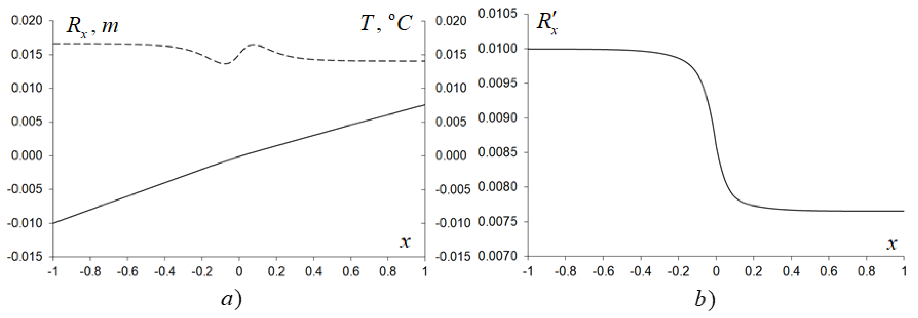
Figure 1 and
Figure 2 show that, on average, the displacement and temperature fields change insignificantly over the fragment under consideration, while the deformations change significantly in a qualitative sense. The change of parameter
changes insignificantly the local temperature field, but changes significantly the local temperature flux fields (
Figure 2a). Note that the gradient theory ensures the continuity of total deformations, but the “semiclassical” part of the deformations breaks at the point of phase contact for all connectivity parameters (see
Figure 3).
In
Figure 4 the Eshelby problem is calculated for the same parameters as in
Figure 1, but with positive
.
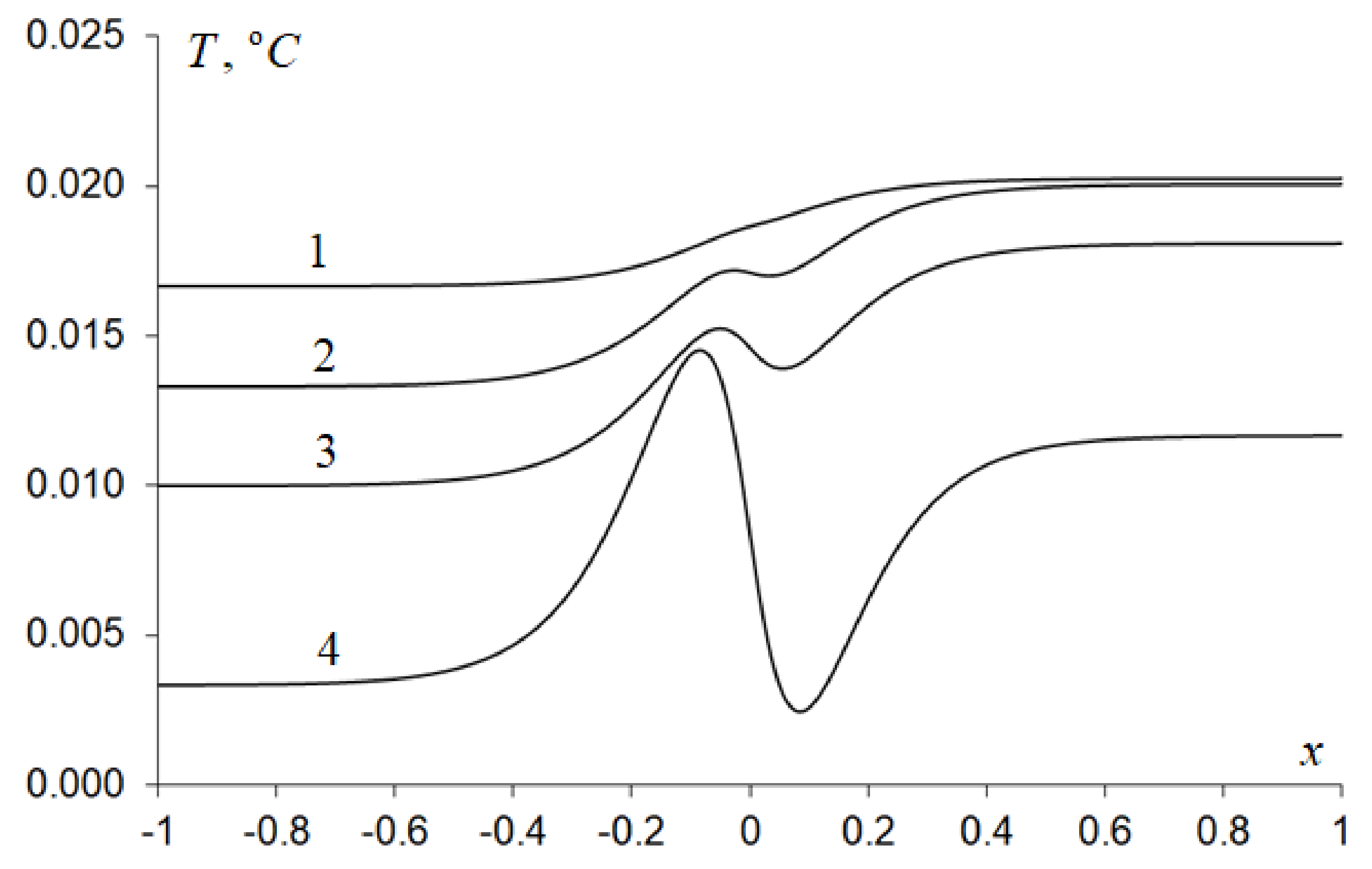
Figure 5 shows the dependences for temperatures at the different parameters
,
and
.
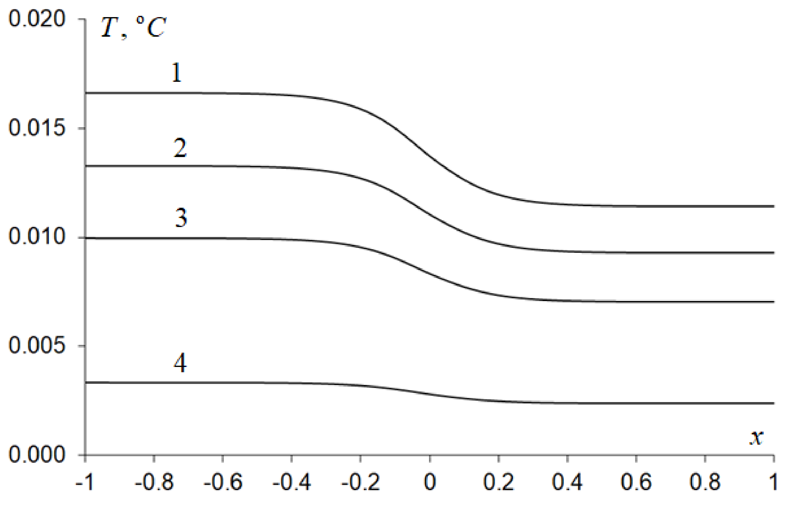
Figure 6 shows the same dependences for
.
The curves of
Figure 4 demonstrate a significant dependence of the mechanical and thermal fields on the connectivity parameter S. Comparison of the results shown in
Figure 1 and
Figure 4 shows that both the displacement fields and especially the temperature fields can vary significantly with the change in the coupled parameter S. These conclusions confirm the dependences shown in
Figure 5, obtained for different values of the parameter S associated with the coefficient of thermal expansion. Comparison of the dependences shown in
Figure 5 and
Figure 6 indicates that the coupled parameters P change, which changes the form of the roots of the characteristic Equation (12), and hence the form of fundamental solutions, which have a special effect on the possible anomalous distribution of local thermal fields in the phase contact zone.
Note that, for the considered case of loading, far from the area of contact between the phases, actually isothermal processes with zero temperature flux are realized; however, in the vicinity of the contacts, significant local heat fluxes arise (see
Figure 1,
Figure 2 and
Figure 3).
The analysis of the Equations (17)–(19) for nonzero roots of the characteristic equation (which takes place for ) shows that the temperature in the Eshelby problem for the deformed two-phase fragment can only have a constant value far from the contact zone. This value of temperature is uniquely related to the deformation field.
The follow statement can be formulated.
Theorem 4. Suppose that and, on the left edge of the layered structure for , only the deformation is given, then the solution for the displacement fields and temperature of the layered system are determined by the Equations (16) and (17) and show that:
1- Far from the contact zone for , a homogeneous deformed equilibrium state with deformation , determined by the parameters of the model, is realized;
2- Far from the contact zone, an isothermal process is realized, which is characterized by a constant temperature equal to .
When , solving the Eshelby problem, the solution for coupled thermoelasticity and stationary thermal conductivity has a nonzero strain value at infinity and the temperature value is associated with this strain by the equation . Moreover, there are no solutions with linear asymptotic of the temperature at infinity (i.e., with a nonzero limiting temperature gradient).
The proof follows directly from Equalities (16) and (17) after passing to the limit for .
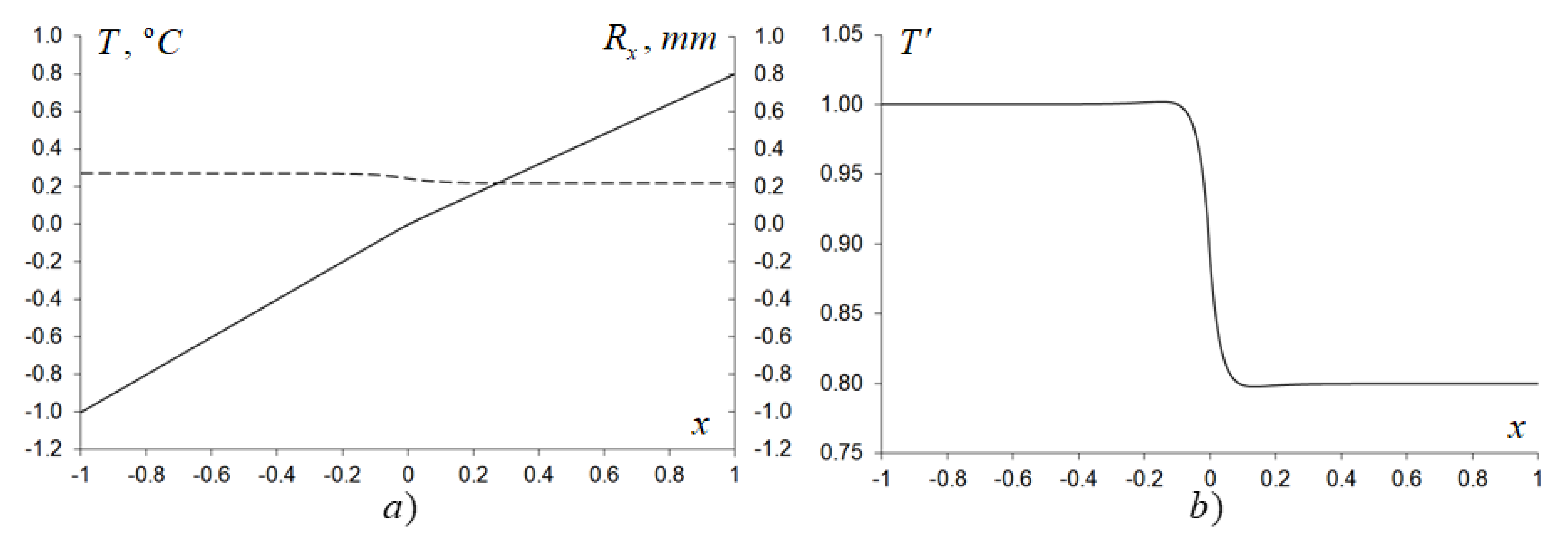
Consider a solution for a two-phase fragment with parameters
when thermal loading occurs. In this case, the solution is represented by relations (25)–(31). As an example,
Figure 7 shows the variant of calculating the Eshelby problem for the coupled gradient thermoelasticity and stationary thermal conductivity with the same parameters as was considered early in
Figure 1, only at
, with a given temperature gradient
and
at the left end of the bar.
As we can see, in this case, the displacement almost does not change and has a constant value at infinity (since zero deformation is obtained at both ends of the bar), and the temperature is close to a linear function. For the complex-valued roots, the solution exhibits similar behavior.
Note also that Equation (25) implies the equality of stresses far from the phase contact, since the temperature does not enter into this equation for (see Theorem 3).
The solutions constructed in
Section 4 and
Section 5 provide the connection between homogeneous states in the left and right phases of the material. It is analogous to the Eshelby tensor in various methods for evaluating the effective characteristics of composite materials (see [
34]). Solutions presented here can also be used to evaluate effective characteristics. In this case, the left-hand phase of the material is treated as a matrix in which a homogeneous state is specified, and the right-hand phase of the material is treated as an inclusion in which this homogeneous state is calculated based on the solution of the Eshelby problem.
The influence of the thermoresistant parameter
on the solution of the problem of coupled gradient thermoelasticity is of great interest.
Figure 8 shows the temperature dependence on the normalized parameter of thermal resistance
in the case
with the same parameters as in
Figure 7.
8. Conclusions
The article provides an analytical solution to the coupled problem of thermoelasticity through harmonic and Helmholtz potentials (in the form of an expansion in fundamental solutions), the structure of which is determined by the scale parameters and coupled parameters of the model. In this solution, in addition to the classical coupled thermoelasticity and the well-known generalizations associated with the consideration of the scale effects of deformation fields, the possible effects of the connectedness of deformation gradients and temperature gradients are also taken into account.
The characteristic numbers that determine the structure of fundamental solutions in general representation are investigated. It is shown that the positive definiteness conditions formulated for the potential energy density of the considered coupled thermoelasticity problem exclude the possibility of the appearance of purely imaginary roots, i.e., there can be no purely oscillating components of the solution. Nevertheless, the consideration of the additional parameter of connectivity of the gradient fields of deformations and temperatures predicts the appearance of rapidly changing temperature fields and significant localized fields of heat fluxes in the vicinity of phase contact in inhomogeneous materials
A transition matrix that determines the relationship between solutions in contacting phases of inhomogeneous structures and provides a formal construction of an algebraic problem corresponding to contact problems for an inhomogeneous material is constructed. On the other hand, the Eshelby matrices connecting homogeneous states far from the contact zone make it possible to assert that, in the general case, these states are not independent. When a homogeneous strain field is specified, the obtained solution predicts a gradient temperature field in the connected problem, which reflects the localization of temperatures and heat fluxes in the vicinity of the phase contact. It is shown that, under certain conditions, when one of the roots of the characteristic equation is equal to zero, a solution that allows setting a homogeneous field of heat fluxes far from the contact zone and describing the localization of deformation fields in the vicinity of the phase contact due to connectivity effects takes place. As a result, the obtained solution makes it possible to study a possible new class of thermomechanical effects that can be realized in the region of phase contact in an inhomogeneous material.
The simulation results presented above are illustrative and demonstrate the possibility of modeling inhomogeneous structures taking into account the coupled effects. Nevertheless, it was found that significant localized heat fluxes can appear in the phase contact area, which largely depend on the model connectivity parameters (
Figure 5 and
Figure 6) and on the thermal resistance characteristics (
Figure 8). Strongly localized heat flux fields, if we follow the Zener thermomechanical damping model [
35], allow, for example, the design of inhomogeneous structures with high damping properties.


