Abstract
One of the major limitations of evolutionary algorithms based on the Lebesgue measure for multi-objective optimization is the computational cost required to approximate the Pareto front of a problem. Nonetheless, the Pareto compliance property of the Lebesgue measure makes it one of the most investigated indicators in the design of indicator-based evolutionary algorithms (IBEAs). The main deficiency of IBEAs that use the Lebesgue measure is their computational cost which increases with the number of objectives of the problem. On this matter, the investigation presented in this paper introduces an evolutionary algorithm based on the Lebesgue measure to deal with box-constrained continuous multi-objective optimization problems. The proposed algorithm implicitly uses the regularity property of continuous multi-objective optimization problems that has suggested effectiveness when solving continuous problems with rough Pareto sets. On the other hand, the survival selection mechanism considers the local property of the Lebesgue measure, thus reducing the computational time in our algorithmic approach. The emerging indicator-based evolutionary algorithm is examined and compared versus three state-of-the-art multi-objective evolutionary algorithms based on the Lebesgue measure. In addition, we validate its performance on a set of artificial test problems with various characteristics, including multimodality, separability, and various Pareto front forms, incorporating concavity, convexity, and discontinuity. For a more exhaustive study, the proposed algorithm is evaluated in three real-world applications having four, five, and seven objective functions whose properties are unknown. We show the high competitiveness of our proposed approach, which, in many cases, improved the state-of-the-art indicator-based evolutionary algorithms on the multi-objective problems adopted in our investigation.
1. Introduction
In several engineering and sciences applications, some problems require the simultaneous optimization of a number of objective functions. In the specialized literature, such problems are referred to as multi-objective optimization problems (MOPs). The optimization of a multi-objective problem involves determining the best compensation alternatives considered in a set of conflicting objective functions. Therefore, instead of an optimal solution, as in single-objective optimization, a set of solutions manifesting the best trade-offs among objectives is reached. The population on which evolutionary algorithms are based makes these algorithms a practical tool to solve these types of problems. For this reason, evolutionary multi-objective algorithms (EMOAs) have become a flexible and popular instrument to deal with MOPs. In the specialized literature, a variety of investigations concerning the development of evolutionary approaches for multi-objective optimization can be found. See the extensive review of such approaches presented in [1,2]. According to their conceptual foundations, EMOAs are categorized into three main groups: Pareto-based, decomposition-based, and indicator-based approaches. These approaches incorporate different search strategies that define by themself the performance of a particular EMOA. Distinctly, EMOAs based on indicators—the topic investigated in this work—explicitly optimize a quality indicator (e.g., [3], Lebesgue measure [4], indicator [5], [6], among others) to approximate the Pareto front of a MOP. In this manner, since its origin in the early 2000s, the indicator-based evolutionary algorithm (IBEA) [7] traced a new research line investigated to date.
IBEAs adopting indicators that use reference sets (e.g., , indicator, , etc.) are a design challenge since the optimal solutions are unknown. Consequently, reference sets cannot be adequately pre-established. Despite this, some researchers have studied diverse techniques to predict the reference set for these IBEAs [8,9]. In the evolutionary multi-objective optimization (EMOO) literature, the Lebesgue measure, also referred to as hypervolume indicator or S-metric, was introduced by Zitzler and Thiele [4] to evaluate the performance of EMOAs. This quality indicator possesses an attractive property—it is Pareto compliant [5]—that has called the attention of several researchers working on IBEAs. In particular, IBEAs adopting the Lebesgue measure benefit from not requiring reference sets because they exclusively employ reference vectors that are much simpler to state. Therefore, these IBEAs have been a practical approach to solving real-life applications where the characteristics of the problems are not known. Although IBEAs based on the Lebesgue measure are highly docile solving MOPs, their application is restricted by the computational cost of the Lebesgue measure, which grows with the number of objective functions. As pointed out in [10], this indicator cannot be calculated in polynomial time concerning the number of objectives except that . In addition, the complex characteristics of multi-objective problems (for example, multimodality, bias, non-separability, etc.) faced by an IBEA, further increase the computational cost in the search process for such algorithms. In other words, IBEAs use many more iterations (computational efforts) to approximate the real Pareto front of a problem. As a consequence, extensive investigations concerning the design of IBEAs using the Lebesgue measure as a quality indicator have been studied in the last few years [11,12,13,14,15]. To date, the development of EMOAs based on the hypervolume indicator is recognized as an actual area of investigation within the EMOO community, and this is precisely the topic of the investigation presented in this work.
This paper introduces an improved Lebesgue indicator-based evolutionary algorithm for multi-objective optimization. The introduced approach can be seen as an improvement of the Lebesgue indicator-based evolutionary algorithm (LIBEA) [15]. Analogous to LIBEA, the proposed algorithm addresses the notion of IBEA [7] in the sense of optimizing a quality indicator. Nevertheless, it is directed at maximizing the Lebesgue measure of non-dominated solutions obtained through the search. In contrast to several Lebesgue indicator-based EMOAs, the introduced algorithm implicitly applies the regularity property of continuous MOPs advised to approximate continuous MOPs with complicated characteristics [16,17,18]. Additionally, in order to reduce the computational time, the local property of the Lebesgue measure is considered in the survival mechanism of the proposed algorithm [19]. We hypothesize that an algorithm considering the Lebesgue measure, the regularity property of continuous MOPs, and the local property of the Lebesgue measure can solve problems with difficult features more efficiently than traditional EMOAs based on the Lebesgue measure.
The proposed IBEA is tested by solving a set of artificial test problems known to be challenging in the EMOO literature. As discussed by some researchers [20], algorithms able to solve test problems having different difficulties can be candidates to deal properly with real-life problems. Consequently, we present an analysis of the proposed algorithm solving three real-life applications where the fitness landscapes and Pareto fronts are unknown. A comparison is carried out to analyze the performance of the suggested IBEA versus three state-of-the-art IBEAs based on the Lebesgue measure. We show that the algorithmic proposal outperforms the state-of-the-art IBEAs in most test problems, including the three real-life problems considered in our study. The obtained results are statistically validated over a number of experiments performed as part of our experimental research.
The rest of the manuscript is organized as follows. Section 2 introduces the fundamental concepts to understand the content of this work. Section 3 introduces an overview of the related work to this investigation. Section 4 introduces the proposed algorithm and details its components. Section 5 presents an experimental study of performance on a set of test problems with complicated features. Section 6 introduces three real-life applications from practice in which the suggested algorithm is tested and analyzed with other IBEAs. Lastly, Section 7 presents our outcomes and describes some paths for future investigation.
2. General Background
This section provides the foundations of multi-objective optimization, introduces the indicator-based multi-objective evolutionary algorithms, and presents some concepts related to performance quality indicators.
2.1. Multi-Objective Optimization
Using standard notation and terminology, a multi-objective optimization problem (MOP) can be defined as follows.
Definition 1
(Multi-objective optimization problem). Without loss of generality, assuming minimization in all the objective functions, a multi-objective optimization problem can be defined as:
where is a solution to the problem, is the solution space, and , for all , are m objective functions. The constraint functions restrict to a feasible region .
In multi-objective optimization, a set of trade-off solutions are normally aimed for, because the minimization of one objective function could lead to the deterioration of the others. To describe the concept of optimality in which we are interested in, the following definitions are presented.
Definition 2
(Pareto dominance). Let . We say that weakly dominates () if for all . If, in addition , we say that strictly dominates (). If for all , we say that strongly dominates ().
Definition 3
(Pareto optimality). Let . We say that is a Pareto optimal solution if there is no other solution such that .
Definition 4
(Pareto optimal set). The Pareto optimal set of a multi-objective problem is defined by is Pareto optimal solution}.
Definition 5
(Pareto optimal front). The Pareto optimal front of a multi-objective problem is stated by the image of the Pareto optimal set, that is, .
An interesting property observed in continuous multi-objective problems that has been considered when designing multi-objective algorithms is presented below.
Property 1
(Regularity property of continuous MOPs). From the Karush–Kuhn–Tucker conditions, it can be induced that under certain assumptions, the () of a continuous MOP with m objectives defines an ()-dimensional piecewise continuous manifold in the decision space (objective space) [21,22].
The regularity property of continuous MOPs defined above was firstly employed by Hillermeier [22] in the well-known continuation methods for multi-objective optimization. As identified by some authors [18], multi-objective solvers should take into account this property explicitly or implicitly.
A critical condition of a multi-objective optimization problem is the conflict among its objectives. If there is no conflict among the objectives, then the problem could be solved by the optimization of each objective function independently. Although several authors have given distinct definitions for the relation between pairs of objectives, the following definition will be used in this paper.
Definition 6
(Conflict relation). Let . According to Carlsson and Fullér [23], two objective functions and can be related in the following three ways (assuming minimization):
- is in conflict with on if ;
- supports on if ;
- and are independent on , otherwise.
2.2. Indicator-Based Evolutionary Algorithms for Multi-Objective Optimization
Quality indicators have been introduced to compare the outcomes of multi-objective algorithms in a quantitative manner. They map a Pareto front approximation to a scalar number that quantifies the performance of a multi-objective approach.
Definition 7
(Quality indicator). An n-ary quality indicator is a function , which assigns each vector of n approximation sets (which can be singletons) a real value .
Currently, we can find a large number of quality indicators for multi-objective optimization. A comprehensive compilation of them can be found in [5,24,25,26]. Quality indicators can assess convergence and diversity of solutions along the Pareto front of a given MOP. However, some indicators require certain knowledge of the problem which, in many cases, is not available. For example, quality indicators based on reference sets (e.g., R2, indicator, IGD, etc.) require a discretization of the entire Pareto front.
Although quality indicators were initially employed for comparison purposes of multi-objective solvers, their use has been extended to guide the optimization process in EMOAs. In this way, with its emergence in the early 2000s, the indicator-based evolutionary algorithm (IBEA) [7] posed the possibility to optimize a quality indicator to approximate the Pareto front of a MOP.
Let us consider the -selection scheme of an EMOA and the combined population of parents and offspring. In order to choose the best solutions for the next population (i.e., the updated set of parents), the fitness assignment to each individual is necessary. Traditionally, EMOAs employ the Pareto ranking and a diversity indicator to update the parents set. The selection mechanism in IBEAs consists of finding the solution that contributes the least to the indicator under consideration. Making allowance for the fitness value of an individual , Algorithm 1 shows the survival selection mechanism in IBEAs.
| Algorithm 1: IBEAs survival selection mechanism. |
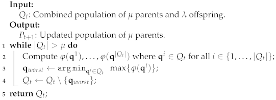 |
In the sense of evolutionary algorithms, the higher the fitness value , the better the individual . Note, however, that according to their conceptual foundations, quality indicators can be either maximized or minimized. Therefore, the adequate fitness values assignment depends directly on the concerned quality indicator. Note that besides the computational time required to estimate the worst solution in IBEAs could be considerably costly (line 2 in Algorithm 1). To date, in the EMOO literature, we can find several evolutionary algorithms based on various quality indicators. A comprehensive review of these types of algorithms can be found in [27].
2.3. Performance Quality Indicators
As pointed out, performance indicators are employed in IBEAs and are also employed to compare performance between algorithms. In the follows, we present some relevant performance indicators in this study.
2.3.1. Hypervolume Performance Indicator
The hypervolume performance indicator, as well known as Lebesgue measure or S metric, has been employed to guide the search in evolutionary algorithms for multi-objective optimization. The follow definitions are relevant in this work [28,29].
Definition 8
(Hypervolume indicator). Let and be a point set and a reference point, respectively. The hypervolume indicator of S is the measure of the region weakly dominated by S and bounded by vector . Formally:
where refers to the Lebesgue measure.
Definition 9
(Hypervolume Contribution). The exclusive hypervolume contribution of a solution to a set respect to the reference vector , is defined as:
The hypervolume contribution of a point is sometimes referred to as Lebesgue contribution, incremental, or exclusive hypervolume contribution. In this regard, some contributions to the state of the art on this topic can be found in [30,31,32].
In the specialized literature, we can find several issues addressed by investigators in relation to the hypervolume indicator, see the comprehensive review on this topic presented in [33]. However, one of the most important challenges in this research area is the exact computation of the hypervolume indicator on a point set S. In this regard, some researchers have designed algorithms that are efficient in a few dimensions, see the works reported in [31,34,35]. The computational complexity of the hypervolume computation is exponential to the number of points in S [19]. An interesting property observed in the two-dimensional objective space that has been exploited for a fast hypervolume computation is presented below.
Property 2
(Locality property of the hypervolume indicator). Given three consecutive points on the Pareto front, moving the middle point will only affect the hypervolume contribution that is solely dedicated to this point, but the joint hypervolume contribution of the other points remains fixed [19].
Nonetheless, the challenges presented in high-dimensional objective spaces have motivated a vast research in the design of algorithms for the efficient hypervolume computation. As a flavor of approaches devoted to the exact hypervolume calculation generalized in the number of dimension, Table 1 presents some algorithms known by the EMOO community and their complexities for an m-dimensional set of n points.

Table 1.
Algorithms for the exact hypervolume computation on an m-dimensional set of n points.
2.3.2. Normalized Hypervolume Indicator
The indicator (stated in Definition 8) can quantify convergence and distribution of solutions on the of a given problem. The normalized hypervolume can be defined as follows.
Definition 10
(Normalized hypervolume indicator). Let and be a point set, an ideal point, and a reference point, respectively, such that (for all ). The normalized hypervolume indicator of S is the measure of the region weakly dominated by S and bounded by vector and . Mathematical it can be stated as:
where denotes the hypervolume indicator of S with reference vector .
The indicator value is in the range . In this way, a large value indicates that the set of solutions S has a suitable approximation and spread on the real .
2.3.3. Indicator
The inverted generational distance plus () [42] is an extension of the indicator [6]. This quality indicator is weakly Pareto compliant and it can quantify how far a given approximation set is from the real Pareto front. Formally, the indicator is stated as follows.
Definition 11
(Inverted Generational Distances plus). Let and be a discretization of the real Pareto front of a given MOP and a set of objective vectors given by an algorithm, respectively. The quality indicator is stated as:
where and is defined by,
where m is the number of objective functions of a given MOP.
A value of zero of the indicator notices that all the objective vectors obtained by an algorithm are on the true .
3. Previous Related Work
The hypervolume indicator (), as well known as Lebesgue or S metric, is a quality indicator widely used to assess the performance of evolutionary multi-objective algorithms [26]. Its peculiar property—it is strictly Pareto compliant [5]—has motivated several investigators working on the design of IBEAs. It has been proved that given a finite search space and a reference point, maximizing the hypervolume indicator is equivalent to finding the Pareto optimal set of a given problem [37]. For this reason, several IBEAs have incorporated this indicator in their survival selection mechanism (see the comprehensive survey of approaches presented in [43]). Lebesgue indicator-based EMOAs need to compute the hypervolume contribution () of non-dominated objective vectors to estimate the worst solution in the current population. As pointed out before, the main disadvantage of the hypervolume indicator is its computation cost which increases exponentially with the number of objectives of the problem. Traditionally, EMOAs based on the indicator need to compute the of each individual in the population per iteration. Examples of these algorithms are SIBEA [44], SMS-EMOA [11], MO-CMA-ES [45], HMOPSO [46], FV-MOEA [14], LIBEA [15], among others. These approaches become impractical when dealing with many objective functions (more than three), employing large populations, or requiring a significant number of generations. Consequently, some authors have focused their investigation on reducing the computational complexity of methods to compute either the or [33,43]. Other alternatives studied by some researchers are the approximation methods to estimate the or [33,43]. In this regard, some authors have incorporated into their IBEAs, approximation methods to calculate . A pioneering study adopting this idea is the HypE algorithm introduced in [47]. Another example of these types of approaches is the R2HCA-EMOA [48], which works similar to SMS-EMOA, but it uses the R2-based hypervolume contribution approximation method [49]. Experimental results presented by the authors show that it outperforms the HypE algorithm in terms of . Although the approximation methods have decreased the computational cost of IBEAs based on the Lebesgue measure, the performance quality in these algorithms is compromised. This is, in effect, the price to compensate for efficiency in these types of IBEAs.
In this paper, we are interested in designing IBEAs based on the exact hypervolume computation. In this regard, Menchaca-Mendéz and Coello [50] presented an improved version of SMS-EMOA called iSMS-EMOA. iSMS-EMOA generates an offspring per iteration. After that, the nearest individual to the offspring (measured by the Euclidean distance in the objective space) and another randomly selected individual compete with the offspring to survive (comparing their ). Therefore, iSMS-EMOA only needs to compute three hypervolume contributions per iteration, unlike SMS-EMOA that calculates n contributions, where n is the population size. The core idea of iSMS-EMOA is to move a solution within its neighborhood to improve its . This idea is based on the locality property stated in [19] (see Property 2). iSMS-EMOA significantly improves the efficiency of SMS-EMOA, and it achieves comparable performance to SMS-EMOA. In [51], the authors studied the behavior of iSMS-EMOA using the approximation method to calculate proposed by Bringmann and Friedrich [52]. The experimental results show that this version of iSMS-EMOA outperforms HypE. In [53], the authors studied the behavior of iSMS-EMOA if it does not use the randomly selected individual in the competition always. Rostami and Neri [54] proposed the algorithm CMA-PAES-HAGA, which incorporates a fast hypervolume-driven selection mechanism for many-objective optimization called HAGA to CMA-ES. HAGA divides the objective space into grids. Then, it separates the population into subpopulations (each grid contains one subpopulation). When a new individual is created, it only competes with the individuals in its grid. Experimental results show that CMA-PAES-HAGA is able to solve problems with more than three objective functions. Recently, Zapotecas-Martínez et al. [15] introduced a novel Lebesgue-based IBEA (LIBEA) adopting the regularity property of continuous MOPs (see Property 1). The introduced LIBEA employs different neighborhoods for the mating selection mechanism. In this way, if a solution is close to the of a problem, it is possible to create new solutions close to the recombining with neighboring solutions. The authors show the effectiveness of LIBEA when solving continuous MOPs with roughed Pareto optimal sets.
In contrast to the related work, we introduce an improved multi-objective solver considering the Lebesgue measure, the regularity property of continuous MOPs, and the local property of the Lebesgue measure. We investigate a new framework to solve problems with difficult features and unknown fitness landscapes more efficiently than traditional IBEAs based on the Lebesgue measure. In the next section, we describe the components of the proposed algorithm thoroughly.
4. Improved Evolutionary Multi-Objective Algorithm Based on the Lebesgue Indicator
The proposed algorithm presented in this paper is an improvement of the Lebesgue indicator-based evolutionary algorithm (LIBEA) [15] for multi-objective optimization. In analogy to LIBEA, the suggested algorithm addresses the notion of IBEA [7] regarding the optimization of a quality indicator. Nevertheless, it is directed at maximizing the Lebesgue indicator of non-dominated solutions obtained through the search. The differences are clearly observed between our algorithmic proposal and IBEAs adopting the Lebesgue measure. This section introduces details of the new algorithm and its components to be compared against state-of-the-art IBEAs.
4.1. Framework of the Improved Lebesgue Indicator-Based Evolutionary Algorithm
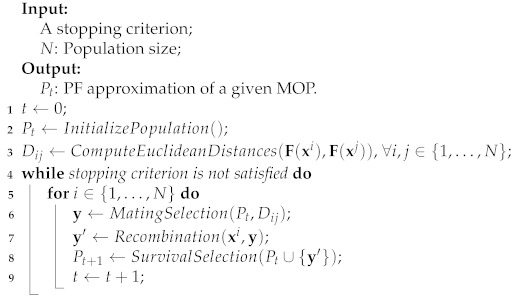
Analogous to its predecessor (LIBEA [15]), the proposed algorithm implicitly adopts the regular property of continuous MOPs to approximate solutions towards the Pareto front of a given problem. The framework of the improved LIBEA (namely here LIBEA-II) is presented in Algorithm 2. Initially, a set of N candidate solutions is generated randomly (Algorithm 2, line 2). A matrix allocating the distances between pairs of objective vectors is calculated and used in the parent selection mechanism of LIBEA-II (Algorithm 2, line 3). At each iteration, for each candidate solution , a parent solution is selected according to the mating selection mechanism (Algorithm 2, line 5). Thus, the recombination procedure is performed by employing the current solution and the parent solution (Algorithm 2, line 6). Section 4.3 illustrates different recombination models that could be adopted into LIBEA-II. Finally, in line 8 of Algorithm 2, a the new population is updated employing the current population and the offspring solution according to the survival selection mechanism described in Section 4.4. In the following, the rest of the components of LIBEA-II are described.
| Algorithm 2: LIBEA-II Framework. |
 |
4.2. Mating Selection Mechanism
The regularity property of continuous MOPs, establish that, under certain conditions, the () of a continuous MOP with m objectives defines an ()-dimensional piecewise continuous manifold in the decision space (objective space) [21,22]. Although this property was firstly introduced by Hillermeier [22] to solve multi-objective problems, its use has been adopted by several EMOAs based on different natures (see for example, the approaches reported in [15,16,17,55,56]). LIBEA-II adopts the regularity property of continuous MOPs in an implicit form by promoting the recombination between neighboring solutions. In this way, if a solution and its neighbors are close to the (), the new offspring solution should also be close to the (). In other words, the local manifold approximated by solution and its neighbors should generate a new solution also close to the (). In the following, the mating selection mechanism of LIBEA-II is described.
Let be the solutions set of the closest solutions to (in the space of the objective functions). LIBEA-II uses a probability to select the solutions set () to be taken into account in the recombination procedure. In the proposed approach, the solutions set is stated by either the neighboring solutions to or the solutions in according to a probability . More precisely:
In this way, the parameter denotes the probability of picking a neighboring solution to be recombined with solution . Otherwise, with probability , any other solution taken from the whole population can be chosen for recombination.
Once the solutions set is stated, a parent solution is chosen randomly from . It is worth noticing that LIBEA-II keeps a distance matrix updated during the search process (we refer to Section 4.4 for more details). Therefore, the solutions set can be computed by employing the partial sorting algorithm [57] with a computational complexity of , such that T denotes the number of desirable solutions in and N represents the number of solutions in .
4.3. Recombination Mechanism
LIBEA-II can be seen as a framework that allows incorporating any recombination mechanism available in the evolutionary computation research area. Nonetheless, it is worth mentioning that for certain recombination operators coming from some meta-heuristics (e.g., PSO [58], DE [59], etc.), consider more than one solution. In such cases, the mating selection mechanism should produce more than one solution for the concerned recombination operator. That is, instead of picking one solution from , various solutions , such that have to be selected. In order to exemplify the mating selection and recombination procedures in the LIBEA-II framework, two popular operators coming from the evolutionary computing field are illustrated below.
Operators from Genetic Algorithms.
Genetic algorithms employ crossover and mutation operators to create offspring solutions throughout the search process. In LIBEA-II, an offspring solution can be created employing such operators according to following equation
where is a solution randomly chosen from , , and are the crossover and mutation operators, respectively. Therefore, LIBEA-II could adopt operators for combinatorial, integer, or mixed optimization.
Operators from Differential Evolution.
A recombination method employed for solving MOPs with difficult [17] exhibiting good results, is the differential evolution (DE) operator [58]. In LIBEA-II, an offspring solution can be created employing DE operator according to the following equation:
such that is the DE crossover, is the perturbed vector, where and are solutions chosen randomly from with, , and F denotes the differential factor, respectively. After performing the DE crossover, a mutation mechanism can be applied to improve the search capabilities, as has been employed by a few researchers [17,18].
4.4. Survival Selection Mechanism
The survival selection mechanism in LIBEA-II (line 8 in Algorithm 2) chooses the best solutions from considering either the Pareto dominance relation or the Lebesgue measure. Since the number of solutions in Q is , it is necessary to remove one solution from Q to make way for the next iteration.
Let and be the number of solutions from Q that dominate solution , and the set of non-dominated solutions in Q, respectively. That is,
Traditionally, IBEAs based on the Lebesgue indicator employ Pareto ranking [60] followed by computing the exclusive Lebesgue contribution (see Definition 2) of each solution allocated in the last rank (see for example the algorithmic proposals introduced in [11,15,61,62]). Therefore, if the last rank contains a large number of solutions, the computational complexity to estimate the solution to be removed becomes extremely high. In evolutionary many-objective optimization, it can be observed that a population constituted by non-dominated solutions can be preserved for several iterations of an algorithm. Therefore, a high computational time is required to decide which solution should be removed from the population. LIBEA-II considers the following two scenarios in the survival selection mechanism.
- If , there are solutions in Q dominated by some solution in . In such a case, we shall remove the solution with the largest value avoiding the Lebesgue measure computation and reducing the computational cost of LIBEA-II;
- If , all solutions in Q are non-dominated, and all of them are equally acceptable in terms of the Pareto dominance relation. In such a case, we shall remove the solution that maximizes the contribution to the Lebesgue measure. In other words, the solution to be removed is the one such that:Therefore, a total of Lebesgue measures are required to identify the worst solution (i.e., the solution that contributes the least to the Lebesgue measure) in the population.
Note that in the case of , the worst solution is found after Lebesgue measures. This is, in fact, computationally expensive and impractical in many-objective optimization problems. LIBEA-II saves Lebesgue measures by reducing the number of candidate solutions in the set S.
A problem observed in IBEAs based on the Lebesgue indicator is the overestimation of the reference vector, which could divert the search. Although the correct estimation of the reference vector for certain types of has been discussed [63], there is no strategy to correctly define this vector for all forms. In such a case, a reference vector close to the nadir vector (the vector opposite the ideal vector) should properly measure the coverage and distribution of solutions along the , including the extreme portions of it. Therefore, the solutions that provide information on the nadir vector should be considered in the survival selection mechanism. In other words, the solutions whose objectives vectors are the farthest to the ideal vector should be considered.
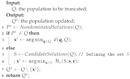
The following criteria to define the set S (line 5 in Algorithm 3) are based on the locality property of the hypervolume indicator studied in [19] (the first three criteria) and the problem to estimate the reference vector for computing the Lebesgue indicator discussed in [63] (the last criterion). The set of candidate solutions S is composed by:
- The offspring solution ;
- The solution such that the objective vector is the closest to the objective vector ;
- A percentage () of solutions which objective vectors are the closest;
- A percentage () of solutions which objective vectors are the farthest to the ideal vector , where the ideal vector is estimated by for all .
In the case that the offspring solution is accepted, it shall replace solution () and the distance matrix has to be updated calculating the Euclidean distances between the objective vector and each objective vector , that is:
In order to deal with different scales (in the objective space), LIBEA-II considers objective vectors normalized in the hypercube bounded by the ideal () and the nadir () vectors. In such cases, the ideal and nadir vectors are defined by the smallest and the largest values of each objective function found in the set of solutions . Therefore, the Lebesgue measure is computed employing the normalized objective vectors and considering the reference vector . In Algorithm 3, we show the complete survival selection mechanism of LIBEA-II.
| Algorithm 3:. |
 |
5. Experimental Study
This section presents the experimental setup and the analysis of results. Firstly, the IBEAs and the benchmark problems adopted for comparison are introduced. Then, the experimental settings are given. Finally, the results on the benchmark problems are analyzed.
5.1. IBEAs Considered for Comparison of Performance
The performance of the proposed LIBEA-II is compared with respect to state-of-the-art IBEAs based on the hypervolume quality indicator. In the first instance, we adopt the S-metric selection EMOA (SMS-EMOA) [11] for performance comparison. SMS-EMO employs a survival mechanism based on Pareto ranking joined by the exclusive Lebesgue contribution of each solution located in the last rank. This evolutionary algorithm has shown its effectiveness and has become popular among state-of-the-art IBEAs. Another algorithm contemplated in this investigation is the improved version of the SMS-EMOA (iSMS-EMOA) [50], which adopts ideas coming from the local property of the hypervolume indicator. Finally, the Lebesgue indicator-based algorithm (LIBEA) [15] for multi-objective optimization is selected. As noticed before, LIBEA adopts the regularity property of continuous MOPs in the mating selection mechanism. Since the proposed LIBEA-II also employs this regularity property, its predecessor, LIBEA, is an obvious competing algorithm.
5.2. Adopted Test Problems
The study presented in this investigation considers the continuous box-constrained MOPs with difficult Pareto sets introduced in [64]. These problems are part of the CEC’2009 competition related to the performance of evolutionary multi-objective algorithms. The adopted test problems have been formulated to assess the performance of EMOAs solving continuous MOPs that exhibit the property of complicated topologies. Since this property has been seen in real-life problems [17], this test suite is a challenge to evaluate the performance of our algorithmic proposal. The adopted test problems (as well known as UFs) offer diverse characteristics regarding separability, multi-modality, and include different shapes, incorporating discontinuities, concavity, convexity, etc. More precisely, we consider the two-objective problems UF1–UF7 and the three-objective problems UF8–UF10.
5.3. Experimental Settings
As pointed out, the results achieved by our proposed algorithm (i.e., LIBEA-II) are analyzed versus those obtained by SMS-EMOA, iSMS-EMOA, and LIBEA on the test problems with roughed (UF1–UF10). As discussed by some authors, MOPs exhibiting complicated shapes shall test specific components of EMOAs, such as the parent selection mechanism and the recombination operators [15,17]. In this work, we use the DE operator whose effectivity has been proved in MOPs with this singular characteristic (see the studies reported in [17]). Therefore, all the IBEAs adopted for performance comparison employ DE operator as their main recombination procedure, such as described in Section 4.3. In order to improve the search capabilities after performing the DE operator, the Polynomial-based mutation [65] is implemented. However, note that for other test problems such as ZDT [66] and DTLZ [67], the performance of IBEAs could be improved by using recombination operators from genetic algorithms, for example, Simulated Binary Crossover (SBX) and Polynomial-based mutation (PBM) [65]. The parameters used by the IBEAs are presented in Table 2, where N denotes the population size. represents the maximum number of generations, in our study . Therefore, the search process was limited to performing 200,000 fitness function evaluations. In the case of the DE operator, F and denote the differential amplitude factor and the crossover rate, which were set as guested in [17] to solve MOPs with complicated . and are the mutation probability and the mutation index used by PBM, respectively. For LIBEA and LIBEA-II, T and are the neighborhood size and the probability of picking solutions from a determined neighborhood (see Section 4.2), respectively. Note that the smaller the value, the effect of the regular property of continuous MOPs is diluted. For LIBEA-II, and are parameters that define the percentage of solutions to be considered in the survival selection mechanism (see Section 4.4). It is worth emphasizing that the smaller these parameters values ( and ), the more efficient LIBEA-II is.
Table 2.
Parameter settings for SMS-EMOA, iSMS-EMOA, LIBEA, and LIBEA-II.
For each IBEA, 30 executions were independently performed on each MOP. The IBEAs were assessed employing the and quality indicators presented in Section 2.3. For each test problem, a statistical analysis was performed over the final approximation produced by the IBEAs in all the experiments using the concerned quality indicator. Since the properties of the UF test functions are known, the quality indicator was calculated by employing the reference vector and the ideal vector . Therefore, a reliable measure of approximation and distribution of solutions obtained by the algorithms along the Pareto front is reported. The indicator was calculated by employing the reference sets provided by the authors of the UF test functions.
5.4. Analysis of Results on the UF Test Problems
The non-dominated solutions found by LIBEA-II, and those from SMS-EMOA, iSMS-EMOA, and LIBEA, to each UF test function, were subjected to the and . Table 3 and Table 4 show the average and values, respectively, over 30 repetitions for each UF problem. These tables have five columns: the first identifies the UF test function, and the remaining four correspond to each of the four algorithms under comparison. The best average and values for each UF problem are in boldface. Moreover, in order to distinguish if there is a statistically significant difference among the average and values for each test function, the Mann–Whitney–Wilcoxon [68] non-parametric statistical test, employing a p-value of , and Bonferroni correction [69] were applied on them. In this manner, an algorithm can be considered the best regarding the test function and quality indicator if it statistically surpasses the other three. If this is the case, the value presented in the Table is underlined.
Table 3.
Average values for the non-dominated solutions found by the IBEAs to each UF test problem.
Table 4.
Average values for the non-dominated solutions found by the IBEAs to each UF test problem.
In Table 3, we can see the average results for the indicator. As we can see, the performance of the four algorithms was very similar: SMS-EMOA obtained the best average results for two test problems, solutions from iSMS-EMOA were the best for one test problem, LIBEA found solutions that were the best to three test problems, and the solutions found by LIBEA-II were the best for three test problems. Actually, these results were expected since all four algorithms are based on the indicator. However, something remarkable is that LIBEA-II was able to find statistically better solutions than those from the other three algorithms for test instance UF8.
quality indicator assesses, to some extent, the closeness and spreading of the non-dominated solutions obtained by an EMOA. Nevertheless, quality indicators based on reference sets could provide more information regarding how distant a set of solutions is from the real . To this end, the indicator was selected to further evaluate the performance of the IBEAs. Table 4 presents the obtained results of the proposed LIBEA-II and those reached by the adopted IBEAs in terms of the indicator. It can be observed that the results achieved by LIBEA-II exceeded those obtained by SMS-EMOA, iSMS-EMOA, and LIBEA in five out of the ten test problems in terms of indicator. LIBEA obtained the best average results in four test problems, while iSMS-EMOA was the best in only one. More importantly, LIBEA-II obtained results that are statistically better than the results from the other three algorithms in problem UF8.
Additionally to the quality indicators, Figure 1 shows the average convergence of the four algorithms under comparison. This figure contains ten plots, one for each UF test function, that show the convergence of the indicator for each algorithm. We can see that the convergence of the indicator is very similar for all four algorithms in each test problem, except for test problem UF7.
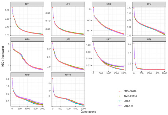
Figure 1.
Convergence plots of the quality indicator on the UF test problems.
After these results, regarding the and quality indicators, we can say that LIBEA-II performs slightly better on the UF test problems than SMS-EMOA, iSMS-EMOA, and LIBEA, since, despite solutions from LIBEA-II, have comparable hypervolumes, they are closer to the in more benchmark functions. Moreover, for the and parameters adopted in this study, LIBEA-II reduces up to approximately the hypervolume indicator calculations, as shown in Figure 2. This means that LIBEA-II is more efficient than the other three algorithms since, with fewer computational resources, it can find solutions with as high quality as those found by SMS-EMOA, iSMS-EMOA, and LIBEA.
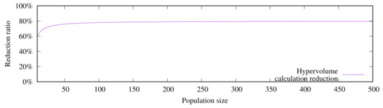
Figure 2.
Reduction of computations in LIBEA-II adopting and .
In order to illustrate the Pareto approximations obtained by the algorithms, Figure 3 presents the non-dominated solutions found by the four algorithms under consideration to the test problems UF1, UF3, and UF7. It is clear that no algorithm could find a proper approximation set to any of the three test problems. However, solutions from SMS-EMOA and LIBEA-II show the best approximations to the Pareto front.
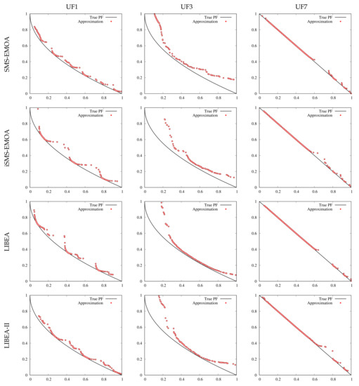
Figure 3.
Non-dominated solutions found by the four algorithms under study to the test problems UF1, UF3, and UF7.
6. Three Real-World Applications from Practice
After testing LIBEA-II on the UF benchmark test problems, it is now tested on three real-world applications. This section introduces, firstly, the three real-world applications under consideration. Secondly, the experimental setup is presented. Thirdly, the results are analyzed. Finally, the correlation between pairs of objectives are analyzed.
6.1. Description of the Real-World Applications
The three real-world applications considered in this study are introduced next.
6.1.1. RWA1: Liquid-Rocket Single Element Injector Design
The design of a liquid-rocket single element injector aims at improving its performance and enlarging its life [70]. Vaidyanathan et al. [71] states that, in order to optimally design such an injector, four objectives should be considered: the maximum injector face temperature (), the wall temperature at a distance of three inches from the injector face (), the maximum oxidizer post tip temperature (), and the centerline axial location where the combustion is 99% complete (). Specifically, this multi-objective optimization problem can be written as:
where , such that is the hydrogen flow angle, is the hydrogen area increment with respect to the baseline cross-section area (), is the oxygen area decrement with respect to the baseline cross-section area () of the tube carrying oxygen, and is the oxidizer post tip thickness, where denotes the tip thickness with a baseline value . The mathematical definition of this problem can be seen in [71].
6.1.2. RWA2: Ultra-Wideband Antenna Design
In order to design an ultra-wideband antenna with two stopbands within the WiMAX and WLAN bands, besides achieving the expected impedance features, gain uniformity and high fidelity are also required [72]. Such antenna comprises a planar rectangular patch and a pair of notches at the two lower corners. Two U-shaped thin slots are carved in the monopole patch for the two stopbands. In order to design this antenna, ten parameters have to be considered and five objective functions, which are the voltage standing wave ratio (VSWR) over the passband (), the VSWR among the WiMAX () and WLAN () bands, respectively, the fidelity factors in the E-plane and H-plane (), and the relatively uniform peak gains over the passband () [73]. Hence, the multi-objective optimization problem is stated as:
where , such that , , , , , , , , , and . The mathematical formulation of this problem is presented in [73].
6.1.3. RWA3: Development of Oil and Water Repellent Fabric
In the textile industry, one aim is to produce fabrics with added high value. Particularly, the hydrophobicity effect, that is, water, oil, and stain repellence, is one of the most widely used textile surface modification [74]. Hydrophobicity depends on several process parameters, such as the concentration of oil and water repellent (O-CPC) finish, the concentration of the crosslinking agent (K-FEL), and the curing temperature (C-Temp) [75]. The hydrophobicity effect can be measured by means of the following seven responses [76]: the contact angle of a water () and oil () droplet touching a surface; the air permeability (), which is the comfort property of a woven fabric used to measure the flow of air through it; the crease recovery angle (), which measures the textiles ability to recover from creasing; the , which is a comfort property of cotton fabric; the of the finished fabric, which depends on the chemical finishing treatment applied to the fabric; and the , which describes the behavior of the fabric under axial stretching load. These seven responses can be considered as objective functions as follows:
where , such that 10 g/L 50 g/L, 10 g/L g/L, and 150 C 170 C. The mathematical description of the problem is presented in [76].
6.2. Experimental Setup
In order to analyze the results achieved by LIBEA-II versus those achieved by SMS-EMOA, iSMS-EMOA, and LIBEA, the following experimental setup was carried out. Since the characteristics of the real-world applications(RWA) described above are not known, the reference had to be constructed to compute the quality indicator .
- The non-dominated solutions obtained by all four IBEAs from the 30 executions were recorded;
- The maximin fitness function [77] was applied to choose 5000 from these non-dominated solutions and they were considered as the reference set for the quality indicator.
Regarding the quality indicator, for each RWA problem, the ideal point was calculated by finding the minimum value for each objective function in the reference . On the other hand, the reference vector was stated by finding the maximum value for each objective function in the reference and scaling its magnitude (with respect to the ideal point) by 10% for each dimension. More precisely, , such that is the maximum value of each objective function in the reference , for all . Hence, the indicator will consider, in a more appropriate scope, the boundaries of the approximation found by each IBEA. Due to the computational cost of the original SMS-EMOA and LIBEA when dealing with more than four objectives, the exact calculation of the was replaced by the HypE indicator [13] employing samples for the approximation, where m denotes the number of objectives in the problem. It is worth noticing that the computational cost of LIBEA-II and the other IBEAs depends directly on the population size and on the number of objectives. Our experimental study adopts solutions to solve the three real-world applications. With this number of solutions, LIBEA-II could deal with problems with up to seven objectives in approximately five days. However, LIBEA-II spent less than 24 h performing a single run for problems having four and five objective functions. The experimental study presented in this work was carried out on a desktop PC with a 32-core 2.6 GHz processor and 64GB of RAM.
6.3. Analysis of Results
The results achieved by LIBEA-II were examined versus those obtained by SMS-EMOA, iSMS-EMOA, and LIBEA. Table 5 and Table 6 show the results achieved by the algorithms in the three real-world applications described above, for the and quality indicators, respectively. The structure of these tables is similar to that of Table 3 and Table 4. That is, the best average and values for each real-world application are in boldface, while the best algorithm regarding the concerned real-world application and quality indicator is underlined.
Table 5.
Average values for the non-dominated solutions found by the IBEAs to each real-world application.
Table 6.
Average values for the non-dominated solutions found by the IBEAs to each real-world application.
Regarding the indicator, we can see from Table 5 that LIBEA-II found solutions that cover a larger hypervolume for the three real-world problems and, remarkably, for problem RWA3, the difference is statistically significant. Concerning the indicator, Table 6 shows that solutions from LIBEA-II obtained, on average, the smallest values for all three real-world problems. In this case, there is a tie between LIBEA-II and iSMS-EMOA for problem RWA1.
Figure 4 shows the average convergence for the indicator. This Figure contains three plots, one for each real-world application. It is evident that the convergence of LIBEA-II is faster than those of the other three algorithms for the two real-world applications RWA1 and RWA3. The convergence for problem RWA2 is similar for all three algorithms.
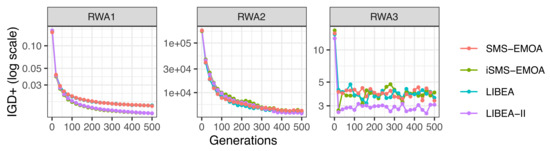
Figure 4.
Convergence of the quality indicator on the three real-world applications.
After these results, it is clear that the performance of LIBEA-II on the three real-world applications is higher than that of SMS-EMOA, iSMS-EMOA, and LIBEA.
6.4. Analysis of the Conflict Relation between Pairs of Objectives
In addition to studying the performance of the four IBEAs on real-world applications, it is also of interest to know the conflict relation (see Definition 5) between the objective functions for each RWA. To this end, Figure 5 presents the parallel coordinates plots for the three real-world applications considered in this study.
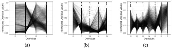
Figure 5.
Parallel coordinate plots for the three real-world applications. (a) RWA1; (b) RWA2; (c) RWA3.
Parallel coordinates are a handy tool for identifying conflict, support, or independence between pairs of objectives. Even though they do not specify information regarding the characteristics of the approximation sets, they are generally utilized for realizing the correlation, whether positive, negative, or neutral, between pairs of objectives [78]. As mentioned earlier, the reference was obtained, for each RWA, by recording all non-dominated solutions found by all four algorithms. For each of these solutions, the values for each objective function were plotted. In Figure 5, the conflict between pairs of objectives is illustrated. This Figure shows three boxes, one for each RWA. For each problem, the objective values are normalized in the vertical axis in the range for a straightforward interpretation, while the objective functions are on the horizontal axis. Lines are plotted from one objective function to the next adjacent to reflect the correlation between the pair of objectives . If a line depicts a significant slope (whether negative or positive) from one objective to the next, it can be interpreted that those objectives are in conflict, and the longer the slope, the greater the conflict. On the contrary, if a line is horizontal, i.e., it has no slope at all, the objectives support each other.
In the case of RWA1, we can see that most of the lines between objectives are nearly horizontal or with a slight slope, which indicates that those objectives support each other. For the pair of objectives , a considerable number of lines have a more significant slope, whether positive or negative, from which we can infer that those objective functions are in conflict. For the last pair , we see that some lines have a slope while others are almost horizontal. Hence, there is no clear conclusion for this pair of objectives.
Following the same analysis as in RWA1, in the case of RWA2, we see that objectives and are clearly in conflict since nearly all the lines present a significant slope and only a few are horizontal or with a slight slope. For the pair of objectives and , on the contrary, most of the lines have a slight slope or are horizontal, while the rest of the lines present a significant slope. For these cases, nothing can be said from these plots.
Finally, for problem RWA3, it is evident that there is conflict for the pairs of objectives , , , and , since the vast majority of the lines presents a significantly large slope, whether positive or negative. For the other two pairs of objectives, and , there is no clear indication whether the objectives are in conflict, support each other, or are independent.
In order to complete the conflict relation analysis between objectives, a numerical analysis of the reference s is presented next. Figure 6 contains three matrices, one for each RWA problem. Each matrix shows: in the upper triangular matrix, the Pearson correlation coefficients [79] between pairs of objectives; in the lower triangular matrix, the projection of the objective function values of the non-dominated solutions between pairs of objectives; and in the diagonal, the densities of each objective function.
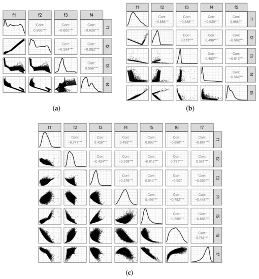
Figure 6.
Pearson correlation coefficients between pairs of objectives for the three RWA problems. (a) RWA1; (b) RWA2; (c) RWA3.
For problem RWA1, we can see that the pairs of objectives and are positively correlated. Remarkably, the correlation for is approximately , which means that optimizing one of them, whether or , will lead to the optimization of the other and vice versa. These results are in accordance with the analysis of the parallel coordinates plots. The remaining four pairs of objectives, i.e., , , , and , present a negative correlation. This means that there is a conflict between the objectives in each pair. That is, the optimization of one objective function deteriorates the other and vice versa.
In the case of problem RWA2, we see a positive correlation for pairs of objectives , , , and , which means that, to some extent, the objectives in each pair support each other. Particularly for the pair , we can observe that the correlation is nearly . The other six pairs of objective functions, that is , , , , , and , present a negative correlation. From these last pairs of objectives, the conflict that exists in and is in agreement with the observed in the parallel coordinates plots.
Finally, for the RWA3 problem, we can confirm what was noticed from the parallel coordinates plots, that is, the pairs of objective functions , , , and presents a negative correlations, which means the objectives in each pair are in conflict with each other. Other pairs of objectives that present a negative correlation are , , , , , , , , and . The remaining eight pairs of objectives show a positive correlation, however, this does not mean that they can be removed from the problem since they show conflict with other objective functions.
7. Conclusions
This paper introduced an improved Lebesgue indicator-based evolutionary algorithm (LIBEA-II) for solving multi-objective optimization problems. The hypothesis put forward in this paper about the efficiency of IBEAs considering the Lebesgue measure, the regularity property of continuous MOPs, and the local property was held. In terms of results, the proposed LIBEA-II and the other three IBEAs, namely SMS-EMOA, iSMS-EMOA, and LIBEA, were tested on the well-known UF benchmark set. These test functions have properties that have been seen in real-life optimization problems in terms of separability, multi-modality, and different shapes, including convexity, concavity, discontinuities, etc. The non-dominated solutions achieved by LIBEA-II and by the other three algorithms, for each test function, were applied the two quality indicators: normalized hypervolume () and inverted generational distance plus (). Results from the indicator showed that the performance of the four algorithms is similar. Given that all four algorithms are based on the quality indicator, this result was rather expected. Regarding the indicator, the performance of LIBEA-II was slightly better than the other three algorithms since it obtained the best average results for five out of the ten test functions, and the difference was statistically significant for one of them. In general, LIBEA-II is an efficient algorithm since it can find solutions with the same quality as those found by the other three algorithms but using only 20% of the computing resources.
LIBEA-II was also tested on three real-world applications, precisely: the liquid-rocket single element injector design (RWA1), which has four objective functions and four variables, the ultra-wideband antenna design (RWA2), which considers five objective functions and ten variables, and the development of oil and water repellent fabric (RWA3), which optimizes seven objective functions with three variables. In this case, LIBEA-II was also compared with the same IBEAs used for the UF test instances. Remarkably, LIBEA-II was able to obtain non-dominated solutions with higher quality than those found by the other three IBEAs, since the average value from both quality indicators, i.e., and , was the best. The superiority of LIBEA-II was demonstrated in real-world applications since it obtained higher-quality non-dominated solutions and saved up to approximately 80% of the hypervolume calculations.
As part of our future research, we are interested in extending the applicability of LIBEA-II to deal with constrained MOPs. This line of research has been slightly explored, and it is the course of our outcoming investigations. On the other hand, we would like to test the performance of the proposed LIBEA-II in other real-life applications in order to identify insights that allow us to understand the main weaknesses of IBEAs based on the Lebesgue measure. On the other hand, the hybridization of these types of approaches with mathematical programming is certainly a good path that deserves to be investigated. These are, in fact, part of our future program of investigations.
Author Contributions
Conceptualization, S.Z.-M.; methodology, S.Z.-M.; software, S.Z.-M. and A.M.-M.; validation, S.Z.-M., A.G.-N.; formal analysis, S.Z.-M. and A.G.-N.; investigation, S.Z.-M., A.M.-M., and A.G.-N.; data curation, S.Z.-M.; writing—original draft preparation, S.Z.-M., A.M.-M., and A.G.-N.; writing—review and editing, S.Z.-M. and A.G.-N.; visualization, S.Z.-M. All authors have read and agreed to the published version of the manuscript.
Funding
This research received no external funding.
Institutional Review Board Statement
Not applicable.
Informed Consent Statement
Not applicable.
Conflicts of Interest
The authors declare no conflict of interest.
References
- Zhou, A.; Qu, B.Y.; Li, H.; Zhao, S.Z.; Suganthan, P.N.; Zhang, Q. Multiobjective evolutionary algorithms: A survey of the state of the art. Swarm Evol. Comput. 2011, 1, 32–49. [Google Scholar] [CrossRef]
- Nedjah, N.; de Macedo Mourelle, L. Evolutionary multi-objective optimisation: A survey. Int. J. -Bio-Inspired Comput. 2015, 7, 1–25. [Google Scholar] [CrossRef]
- Hansen, M.P.; Jaszkiewicz, A. Evaluating the Quality of Approximations to the Non-Dominated Set; Technical Report IMM-REP-1998-7; Technical University of Denmark: Kongens Lyngby, Denmark, 1998. [Google Scholar]
- Zitzler, E.; Thiele, L. Multiobjective Optimization Using Evolutionary Algorithms—A Comparative Study. In Parallel Problem Solving from Nature V; Eiben, A.E., Ed.; Springer: Amsterdam, The Netherlands, 1998; pp. 292–301. [Google Scholar]
- Zitzler, E.; Thiele, L.; Laumanns, M.; Fonseca, C.M.; da Fonseca, V.G. Performance Assessment of Multiobjective Optimizers: An Analysis and Review. IEEE Trans. Evol. Comput. 2003, 7, 117–132. [Google Scholar] [CrossRef] [Green Version]
- Coello, C.A.C.; Reyes Sierra, M. A Study of the Parallelization of a Coevolutionary Multi-Objective Evolutionary Algorithm. In Proceedings of the Third Mexican International Conference on Artificial Intelligence (MICAI’2004), Mexico City, Mexico, 26–30 April 2004; Monroy, R., Arroyo-Figueroa, G., Sucar, L.E., Sossa, H., Eds.; Lecture Notes in Artificial Intelligence; Springer: Amsterdam, The Netherlands, 2004; Volume 2972, pp. 688–697. [Google Scholar]
- Zitzler, E.; Künzli, S. Indicator-based Selection in Multiobjective Search. In Parallel Problem Solving from Nature—PPSN VIII; Lecture Notes in Computer Science; Springer: Amsterdam, The Netherlands, 2004; Volume 3242, pp. 832–842. [Google Scholar]
- Rodríguez Villalobos, C.A.; Coello, C.A.C. A new multi-objective evolutionary algorithm based on a performance assessment indicator. In Proceedings of the GECCO’2012, Philadelphia, PA, USA, 7–11 July 2012; ACM: New York, NY, USA, 2012; pp. 505–512. [Google Scholar]
- Zapotecas Martínez, S.; Sosa Hernández, V.A.; Aguirre, H.; Tanaka, K.; Coello Coello, C.A. Using a Family of Curves to Approximate the Pareto Front of a Multi-Objective Optimization Problem. In Parallel Problem Solving from Nature—PPSN XIII, Proceedings of the 13th International Conference, Ljubljana, Slovenia, 13–17 September 2014; Bartz-Beielstein, T., Branke, J., Filipič, B., Smith, J., Eds.; Lecture Notes in Computer Science; Springer: Amsterdam, The Netherlands, 2014; Volume 8672, pp. 682–691. [Google Scholar]
- Bringmann, K.; Friedrich, T. Approximating the Least Hypervolume Contributor: NP-Hard in General, But Fast in Practice. In Evolutionary Multi-Criterion Optimization, Proceedings of the 5th International Conference, EMO 2009, Nantes, France, 7–10 April 2009; Ehrgott, M., Fonseca, C.M., Gandibleux, X., Hao, J.K., Sevaux, M., Eds.; Lecture Notes in Computer Science; Springer: Amsterdam, The Netherlands, 2009; Volume 5467, pp. 6–20. [Google Scholar]
- Beume, N.; Naujoks, B.; Emmerich, M. SMS-EMOA: Multiobjective selection based on dominated hypervolume. Eur. J. Oper. Res. 2007, 181, 1653–1669. [Google Scholar] [CrossRef]
- Tsukamoto, N.; Sakane, Y.; Nojima, Y.; Ishibuchi, H. Incorporation of Hypervolume Approximation with Scalarizing Functions into Indicator-based Evolutionary Multiobjective Optimization Algorithms. Trans. Inst. Syst. Control Inf. Eng. 2010, 23, 165–177. [Google Scholar]
- Bader, J.; Deb, K.; Zitzler, E. Faster Hypervolume-Based Search Using Monte Carlo Sampling. In Multiple Criteria Decision Making for Sustainable Energy and Transportation Systems; Ehrgott, M., Naujoks, B., Stewart, T.J., Wallenius, J., Eds.; Lecture Notes in Economics and Mathematical Systems; Springer: Amsterdam, The Netherlands, 2010; Volume 634, pp. 313–326. [Google Scholar]
- Jiang, S.; Zhang, J.; Ong, Y.S.; Zhang, A.N.; Tan, P.S. A Simple and Fast Hypervolume Indicator-Based Multiobjective Evolutionary Algorithm. IEEE Trans. Cybern. 2015, 45, 2202–2213. [Google Scholar] [CrossRef]
- Zapotecas-Martínez, S.; García-Nájera, A.; López-Jaimes, A. LIBEA: A Lebesgue Indicator-Based Evolutionary Algorithm for multi-objective optimization. Swarm Evol. Comput. 2019, 44, 404–419. [Google Scholar] [CrossRef]
- Zhang, Q.; Li, H. MOEA/D: A Multiobjective Evolutionary Algorithm Based on Decomposition. IEEE Trans. Evol. Comput. 2007, 11, 712–731. [Google Scholar] [CrossRef]
- Li, H.; Zhang, Q. Multiobjective Optimization Problems With Complicated Pareto Sets, MOEA/D and NSGA-II. IEEE Trans. Evol. Comput. 2009, 13, 284–302. [Google Scholar] [CrossRef]
- Zhou, A.; Zhang, Q.; Zhang, G. A multiobjective evolutionary algorithm based on decomposition and probability model. In Proceedings of the 2012 IEEE Congress on Evolutionary Computation (CEC’2012), Brisbane, QLD, Australia, 10–15 June 2012; IEEE Press: Brisbane, Australia, 2012; pp. 3151–3158. [Google Scholar]
- Auger, A.; Bader, J.; Brockhoff, D.; Zitzler, E. Theory of the Hypervolume Indicator: Optimal {μ}-Distributions and the Choice Of The Reference Point. In Proceedings of the FOGA ’09: Tenth ACM SIGEVO Workshop on Foundations of Genetic Algorithms, Orlando, FL, USA, 9–11 January 2009; ACM: Orlando, FL, USA, 2009; pp. 87–102. [Google Scholar]
- Chand, S.; Wagner, M. Evolutionary many-objective optimization: A quick-start guide. Surv. Oper. Res. Manag. Sci. 2015, 20, 35–42. [Google Scholar] [CrossRef] [Green Version]
- Miettinen, K. Nonlinear Multiobjective Optimization; Kluwer Academic Publishers: Boston, MA, USA, 1999. [Google Scholar]
- Hillermeier, C. Nonlinear Multiobjective Optimization—A Generalized Homotopy Approach; Birkhaäuser: Basel, Switzerland, 2001. [Google Scholar]
- Carlsson, C.; Fullér, R. Multiple criteria decision making: The case for interdependence. Comput. Oper. Res. 1995, 22, 251–260. [Google Scholar] [CrossRef]
- Okabe, T.; Jin, Y.; Sendhoff, B. A Critical Survey of Performance Indices for Multi-Objective Optimization. In Proceedings of the 2003 Congress on Evolutionary Computation (CEC’2003), Canberra, Australia, 8–12 December 2003; IEEE Press: Canberra, Australia, 2003; Volume 2, pp. 878–885. [Google Scholar]
- Jiang, S.; Ong, Y.S.; Zhang, J.; Feng, L. Consistencies and Contradictions of Performance Metrics in Multiobjective Optimization. IEEE Trans. Cybern. 2014, 44, 2391–2404. [Google Scholar] [CrossRef]
- Li, M.; Yao, X. Quality Evaluation of Solution Sets in Multiobjective Optimisation: A Survey. ACM Comput. Surv. 2019, 52, 1–38. [Google Scholar] [CrossRef]
- Falcón-Cardona, J.G.; Coello, C.A.C. Indicator-Based Multi-Objective Evolutionary Algorithms: A Comprehensive Survey. ACM Comput. Surv. 2020, 53, 1–35. [Google Scholar] [CrossRef] [Green Version]
- Knowles, J.; Corne, D.; Fleischer, M. Bounded archiving using the lebesgue measure. In Proceedings of the 2003 Congress on Evolutionary Computation, 2003 CEC ’03, Canberra, ACT, Australia, 8–12 December 2003; Volume 4, pp. 2490–2497. [Google Scholar] [CrossRef]
- While, L.; Bradstreet, L. Applying the WFG algorithm to calculate incremental hypervolumes. In Proceedings of the 2012 IEEE Congress on Evolutionary Computation, Brisbane, QLD, Australia, 10–15 June 2012; pp. 1–8. [Google Scholar] [CrossRef]
- Emmerich, M.T.; Fonseca, C.M. Computing hypervolume contributions in low dimensions: Asymptotically optimal algorithm and complexity results. In International Conference on Evolutionary Multi-criterion Optimization; Springer: Berlin/Heidelberg, Germany, 2011; pp. 121–135. [Google Scholar]
- Guerreiro, A.P.; Fonseca, C.M. Computing and updating hypervolume contributions in up to four dimensions. IEEE Trans. Evol. Comput. 2017, 22, 449–463. [Google Scholar] [CrossRef]
- Russo, L.M.; Francisco, A.P. Extending quick hypervolume. J. Heuristics 2016, 22, 245–271. [Google Scholar] [CrossRef]
- Guerreiro, A.P.; Fonseca, C.M.; Paquete, L. The Hypervolume Indicator: Computational Problems and Algorithms. ACM Comput. Surv. 2021, 54, 119. [Google Scholar] [CrossRef]
- Beume, N.; Fonseca, C.M.; Lopez-Ibanez, M.; Paquete, L.; Vahrenhold, J. On the complexity of computing the hypervolume indicator. IEEE Trans. Evol. Comput. 2009, 13, 1075–1082. [Google Scholar] [CrossRef] [Green Version]
- Guerreiro, A.P.; Fonseca, C.M.; Emmerich, M.T. A Fast Dimension-Sweep Algorithm for the Hypervolume Indicator in Four Dimensions. In Proceedings of the Canadian Conference on Computational Geometry, Charlottetown, PEI, Canada, 8–10 August 2012; pp. 77–82. [Google Scholar]
- Knowles, J.D. Local-Search and Hybrid Evolutionary Algorithms for Pareto Optimization. Ph.D. Thesis, University of Reading, Reading, UK, 2002. [Google Scholar]
- Fleischer, M. The measure of Pareto optima applications to multi-objective metaheuristics. In International Conference on Evolutionary Multi-Criterion Optimization; Springer: Berlin/Heidelberg, Germany, 2003; pp. 519–533. [Google Scholar]
- Fonseca, C.M.; Paquete, L.; López-Ibánez, M. An improved dimension-sweep algorithm for the hypervolume indicator. In Proceedings of the 2006 IEEE International Conference on Evolutionary Computation, Vancouver, BC, Canada, 16–21 July 2006; pp. 1157–1163. [Google Scholar]
- Beume, N. S-metric calculation by considering dominated hypervolume as Klee’s measure problem. Evol. Comput. 2009, 17, 477–492. [Google Scholar] [CrossRef]
- While, L.; Bradstreet, L.; Barone, L. A fast way of calculating exact hypervolumes. IEEE Trans. Evol. Comput. 2011, 16, 86–95. [Google Scholar] [CrossRef]
- Russo, L.M.; Francisco, A.P. Quick hypervolume. IEEE Trans. Evol. Comput. 2013, 18, 481–502. [Google Scholar] [CrossRef]
- Ishibuchi, H.; Masuda, H.; Tanigaki, Y.; Nojima, Y. Modified Distance Calculation in Generational Distance and Inverted Generational Distance. In Evolutionary Multi-Criterion Optimization, Proceedings of the 8th International Conference, EMO 2015, Guimarães, Portugal, 29 March–1 April 2015; Gaspar-Cunha, A., Antunes, C.H., Coello Coello, C., Eds.; Lecture Notes in Computer Science; Springer: Amsterdam, The Netherlands, 2015; Volume 9019, pp. 110–125. [Google Scholar]
- Shang, K.; Ishibuchi, H.; He, L.; Pang, L.M. A Survey on the Hypervolume Indicator in Evolutionary Multiobjective Optimization. IEEE Trans. Evol. Comput. 2021, 25, 1–20. [Google Scholar] [CrossRef]
- Zitzler, E.; Brockhoff, D.; Thiele, L. The Hypervolume Indicator Revisited: On the Design of Pareto-compliant Indicators Via Weighted Integration. In Evolutionary Multi-Criterion Optimization; Obayashi, S., Deb, K., Poloni, C., Hiroyasu, T., Murata, T., Eds.; Springer: Berlin/Heidelberg, Germany, 2007; pp. 862–876. [Google Scholar]
- Igel, C.; Hansen, N.; Roth, S. Covariance Matrix Adaptation for Multi-objective Optimization. Evol. Comput. 2007, 15, 1–28. [Google Scholar] [CrossRef]
- Mostaghim, S.; Branke, J.; Schmeck, H. Multi-Objective Particle Swarm Optimization on Computer Grids. In Proceedings of the 9th Annual Conference on Genetic and Evolutionary Computation, London, UK, 7–11 July 2007; Association for Computing Machinery: New York, NY, USA, 2007; pp. 869–875. [Google Scholar] [CrossRef] [Green Version]
- Bader, J.; Zitzler, E. HypE: An Algorithm for Fast Hypervolume-Based Many-Objective Optimization. Evol. Comput. 2011, 19, 45–76. [Google Scholar] [CrossRef]
- Shang, K.; Ishibuchi, H. A New Hypervolume-Based Evolutionary Algorithm for Many-Objective Optimization. IEEE Trans. Evol. Comput. 2020, 24, 839–852. [Google Scholar] [CrossRef]
- Shang, K.; Ishibuchi, H.; Ni, X. R2-Based Hypervolume Contribution Approximation. IEEE Trans. Evol. Comput. 2020, 24, 185–192. [Google Scholar] [CrossRef] [Green Version]
- Menchaca-Mendéz, A.; Coello, C.A.C. A new selection mechanism based on hypervolume and its locality property. In Proceedings of the 2013 IEEE Congress on Evolutionary Computation, Cancún, México, 20–23 June 2013; pp. 924–931. [Google Scholar] [CrossRef]
- Menchaca-Mendez, A.; Coello Coello, C.A. An alternative hypervolume-based selection mechanism for multi-objective evolutionary algorithms. Soft Comput. 2017, 21, 861–884. [Google Scholar] [CrossRef]
- Bringmann, K.; Friedrich, T. Approximating the least hypervolume contributor: NP-hard in general, but fast in practice. Theor. Comput. Sci. 2012, 425, 104–116. [Google Scholar] [CrossRef] [Green Version]
- Menchaca-Méndez, A.; Montero, E.; Zapotecas-Martínez, S. An Improved S-Metric Selection Evolutionary Multi-Objective Algorithm With Adaptive Resource Allocation. IEEE Access 2018, 6, 63382–63401. [Google Scholar] [CrossRef]
- Rostami, S.; Neri, F. Covariance matrix adaptation pareto archived evolution strategy with hypervolume-sorted adaptive grid algorithm. Integr. Comput.-Aided Eng. 2016, 23, 313–329. [Google Scholar] [CrossRef] [Green Version]
- Zhang, Q.; Zhou, A.; Jin, Y. RM-MEDA: A Regularity Model-Based Multiobjective Estimation of Distribution Algorithm. IEEE Trans. Evol. Comput. 2008, 12, 41–63. [Google Scholar] [CrossRef] [Green Version]
- Schütze, O.; Coello Coello, C.A.; Mostaghim, S.; Talbi, E.G.; Dellnitz, M. Hybridizing evolutionary strategies with continuation methods for solving multi-objective problems. Eng. Optim. 2008, 40, 383–402. [Google Scholar] [CrossRef]
- Chambers, J.M. Algorithm 410: Partial Sorting. Commun. ACM 1971, 14, 357–358. [Google Scholar] [CrossRef]
- Kennedy, J.; Eberhart, R.C. Particle swarm optimization. In Proceedings of the IEEE International Conference on Neural Networks, Perth, WA, Australia, 27 November–1 December 1995; pp. 1942–1948. [Google Scholar]
- Storn, R.M.; Price, K.V. Differential Evolution—A Simple and Efficient Adaptive Scheme for Global Optimization over Continuous Spaces; Technical Report TR-95-012; International Computer Science Institute: Berkeley, CA, USA, 1995. [Google Scholar]
- Goldberg, D.E. Genetic Algorithms in Search, Optimization and Machine Learning; Addison-Wesley Publishing Company: Reading, MA, USA, 1989. [Google Scholar]
- Knowles, J.; Corne, D. Properties of an Adaptive Archiving Algorithm for Storing Nondominated Vectors. IEEE Trans. Evol. Comput. 2003, 7, 100–116. [Google Scholar] [CrossRef]
- Huband, S.; Hingston, P.; White, L.; Barone, L. An Evolution Strategy with Probabilistic Mutation for Multi-Objective Optimisation. In Proceedings of the 2003 Congress on Evolutionary Computation (CEC’2003), Canberra, Australia, 8–12 December 2003; IEEE Press: Canberra, Australia, 2003; Volume 3, pp. 2284–2291. [Google Scholar]
- Ishibuchi, H.; Imada, R.; Setoguchi, Y.; Nojima, Y. Reference Point Specification in Hypervolume Calculation for Fair Comparison and Efficient Search. In Proceedings of the Genetic and Evolutionary Computation Conference, Berlin, Germany, 15–19 July 2017; Association for Computing Machinery: New York, NY, USA, 2017; pp. 585–592. [Google Scholar] [CrossRef]
- Zhang, Q.; Zhou, A.; Zhao, S.; Suganthan, P.N.; Liu, W.; Tiwari, S. Multiobjective Optimization Test Instances for the CEC 2009 Special Session and Competition. In Special Session on Performance Assessment of Multi-Objective Optimization Algorithms; Technical Report CES-487; University of Essex: Colchester, UK; Nanyang Technological University: Singapore, 2008; Volume 264. [Google Scholar]
- Deb, K.; Pratap, A.; Agarwal, S.; Meyarivan, T. A Fast and Elitist Multiobjective Genetic Algorithm: NSGA–II. IEEE Trans. Evol. Comput. 2002, 6, 182–197. [Google Scholar] [CrossRef] [Green Version]
- Zitzler, E.; Deb, K.; Thiele, L. Comparison of Multiobjective Evolutionary Algorithms: Empirical Results. Evol. Comput. 2000, 8, 173–195. [Google Scholar] [CrossRef] [Green Version]
- Deb, K.; Thiele, L.; Laumanns, M.; Zitzler, E. Scalable Multi-Objective Optimization Test Problems. In Proceedings of the Congress on Evolutionary Computation (CEC’2002), Honolulu, HI, USA, 12–17 May 2002; IEEE Service Center: Piscataway, NJ, USA, 2002; Volume 1, pp. 825–830. [Google Scholar]
- Wilcoxon, F. Individual Comparisons by Ranking Methods. Biom. Bull. 1945, 1, 80–83. [Google Scholar] [CrossRef]
- Bonferroni, C.E. Teoria statistica delle classi e calcolo delle probabilita. Pubbl. R Ist. Super. Sci. Econ. Commer. Firenze 1936, 8, 3–62. [Google Scholar]
- Goel, T.; Vaidyanathan, R.; Haftka, R.T.; Shyy, W.; Queipo, N.V.; Tucker, K. Response surface approximation of Pareto optimal front in multi-objective optimization. Comput. Methods Appl. Mech. Eng. 2007, 196, 879–893. [Google Scholar] [CrossRef]
- Vaidyanathan, R.; Tucker, P.K.; Papila, N.; Shyy, W. Computational-fluid-dynamics-based design optimization for single-element rocket injector. J. Propuls. Power 2004, 20, 705–717. [Google Scholar] [CrossRef]
- Chen, Y.S. Performance enhancement of multiband antennas through a two-stage optimization technique. Int. J. Microw.-Comput.-Aided Eng. 2017, 27, e21064. [Google Scholar] [CrossRef]
- Chen, Y.S. Multiobjective optimization of complex antenna structures using response surface models. Int. J. Microw. Comput.-Aided Eng. 2016, 26, 62–71. [Google Scholar] [CrossRef]
- Genzer, J.; Marmur, A. Biological and synthetic self-cleaning surfaces. MRS Bull. 2008, 33, 742–746. [Google Scholar] [CrossRef] [Green Version]
- Sun, T.; Feng, L.; Gao, X.; Jiang, L. Bioinspired surfaces with special wettability. Accounts Chem. Res. 2005, 38, 644–652. [Google Scholar] [CrossRef] [PubMed]
- Ahmad, N.; Kamal, S.; Raza, Z.A.; Hussain, T. Multi-objective optimization in the development of oil and water repellent cellulose fabric based on response surface methodology and the desirability function. Mater. Res. Express 2017, 4, 035302. [Google Scholar] [CrossRef]
- Balling, R. The maximin fitness function for multiobjective evolutionary optimization. In Optimization in Industry; Springer: Berlin/Heidelberg, Germany, 2002; pp. 135–147. [Google Scholar]
- Tušar, T.; Filipič, B. Visualization of Pareto Front Approximations in Evolutionary Multiobjective Optimization: A Critical Review and the Prosection Method. IEEE Trans. Evol. Comput. 2015, 19, 225–245. [Google Scholar] [CrossRef]
- Pearson, K. Notes on regression and inheritance in the case of two parents. Proc. R. Soc. Lond. 1895, 58, 240–242. [Google Scholar]
Publisher’s Note: MDPI stays neutral with regard to jurisdictional claims in published maps and institutional affiliations. |
© 2021 by the authors. Licensee MDPI, Basel, Switzerland. This article is an open access article distributed under the terms and conditions of the Creative Commons Attribution (CC BY) license (https://creativecommons.org/licenses/by/4.0/).