Closing a Bitcoin Trade Optimally under Partial Information: Performance Assessment of a Stochastic Disorder Model

Abstract

The Bitcoin market exhibits characteristics of a market with pricing bubbles. The price is very volatile, and it inherits the risk of quickly increasing to a peak and decreasing from the peak even faster. In this context, it is vital for investors to close their long positions optimally. In this study, we investigate the performance of the partially observable digital-drift model of Ekström and Lindberg and the corresponding optimal exit strategy on a Bitcoin trade. In order to estimate the unknown intensity of the random drift change time, we refer to Bitcoin halving events, which are considered as pivotal events that push the price up. The out-of-sample performance analysis of the model yields returns values ranging between 9% and 1153%. We conclude that the return of the initiated Bitcoin momentum trades heavily depends on the entry date: the earlier we entered, the higher the expected return at the optimal exit time suggested by the model. Overall, to the extent of our analysis, the model provides a supporting framework for exit decisions, but is by far not the ultimate tool to succeed in every trade.

1. Introduction

“Buy low and sell high” is the common advice given to rational investors. The advice is easier to follow in the markets where the asset prices move primarily according to the underlying fundamentals. However, in the case of financial bubbles, asset price increases are mainly due to the belief that future prices will increase, known as the so-called momentum effect. In that case, following the advice becomes more challenging, and trading becomes riskier, as it becomes harder to predict the ultimate maximum, which would be exactly known only after the bubble bursts.

The cryptocurrency market has attracted significant attention over the past few years, leading to abnormal returns for early investors. Bitcoin was officially launched on 3 January 2009, when the first block of the Bitcoin blockchain, called the genesis block, was created. Over the years, Bitcoin has become the best performing asset ever, reaching approximately 28,000 percent of a return on investment. Among the cryptocurrency community, keywords like “HODL”, which means “Hold on, doubt less”, or “FOMO”, which means “Fear of missing out”, established, referring to the extreme market dynamics of cryptocurrencies. A 10 percent loss on a given day is accepted as normal in the cryptocurrency market, while such a drop would lead to financial turmoil in traditional markets, such as a stock market.

Moreover, momentum seems to exist in cryptocurrencies (see, e.g., [1,2]), which might be due to the herding effect ([3]). Overall, the cryptocurrency market and markets with a speculative bubble share some common characteristics, like being very volatile and inheriting the risk of quickly increasing to a peak, and decreasing from the peak in an even quicker way (see, [4,5], for an extensive review on the properties of the cryptocurrency market). In this context, it is vital for small investors to determine the closing time of their positions optimally. Not doing so may prevent investors from using the momentum opportunity, and may result in significant losses in a short period, mainly due to the fast-moving property of the Bitcoin price.

Acknowledging the stylized facts of the markets with a financial bubble, refs. [6,7,8] propose a partial-information setting, and analyze how to close long and short positions optimally in a momentum trade in the market with bubbles. Both studies modeled the underlying asset price as a geometric Brownian motion with disorder. That is, the drift of the return process is governed by a random variable that can take only two values, yielding a positive drift or a negative drift, which is not directly observable by the investor. The investor is assumed to observe prices and know the distribution of the random time that the drift changes from a positive value to a negative one. What distinguishes the settings given in [6] and ref. [7] is the underlying assumption on the distribution of the random time that the drift change occurs: the former study assumes an exponentially distributed random time, and the latter assumes that the random time is uniformly distributed. While the exponential distribution assumption implies that the bubble will burst or the momentum effect will vanish in time, the uniform distribution assumption suggests maximum uncertainty on the actual structure of the distribution of the random time, since the uniform distribution has the maximum entropy on a finite time interval.

The investor’s objective is to maximize the profit from the trade, and accordingly, he or she would hold a long position until the drift changes from the positive to the negative value. As the exact time of the drift change is not known to the investor, he or she faces an optimal stopping problem under incomplete information. As a solution to this problem, ref. [6] characterizes the optimal trading strategy as the closing of the long position at the first time when the conditional probability that the random changing time hits a constant barrier, which is given through the solution of a free boundary problem. The solution provided in [9] is based on the so-called Shiryaev–Roberts statistic (SR), and the optimal closing time is characterized as the first time when the SR process crosses some time-dependent boundary, which can be obtained from a particular integral equation. The model suggested in [7] is shown to perform well in the US stock market data (see [9]), while the performance of the model given in [6] has not been investigated so far.

Several studies have suggested sophisticated models for the Bitcoin price dynamics (see, e.g., [10,11]). Although the proposed models seem to be consistent in explaining the price behavior, they may not be suitable for the analysis we would like to conduct here, assuming that a stochastic or rough volatility model does not allow for a partial information setting in continuous time. In particular, in a rough model, the volatility process is neither a semimartingale nor a Markov process, and accordingly, it is not possible to use standard results in stochastic filtering.

In this paper, our objective is to investigate the performance of the stochastic disorder model introduced in [6]. Although the theoretical results are readily available for the model under consideration, it necessitates an effort to bring them into practice. In particular, estimation of the parameter ($\lambda )$ of the distribution of the random time that the drift change occurs is not straightforward. If we could observe the exact times of the drift changes, $\lambda$ could be estimated by counting the number of drift changes during the estimation period, and dividing this number by the sum of waiting times between two consecutive changes.

We think that the Bitcoin market is suitable to apply the stochastic disorder model due to having many local maxima in the historical price series. Our idea is to use the specific properties of this market to tackle the issue concerning the estimation of $\lambda$. More precisely, to attribute a down (up) movement in an ongoing increase (decrease) in prices to a drift change ex-post, we suggest referring to Bitcoin halving events. Bitcoin halving events occur after 210,000 new blocks are added to the blockchain. Then, the rate at which new coins are released into circulation is cut in half. Thus, Bitcoin miners who receive the newly issued Bitcoins for the computational power they provide to secure and maintain the entire system will only continue to perform their tasks if they are compensated for the remuneration cut. The only way to compensate Bitcoin miners for their "loss” is an immediate price increase of Bitcoin. Hence, after each halving event, a significant price increase is expected at some future point (see Section 2.4 for details). For this reason, we suggest to initiate long Bitcoin trades after each halving event. The recent literature provides results on the detection of cryptocurrency bubbles, see, e.g., [12,13]. By using the log-periodic approach, ref. [13] presents a detailed bubble analysis of the Bitcoin, and identify three major peaks and ten additional smaller peaks. We mainly cover the periods with major bubbles in our analysis below.

Following [9], we suggest a drift parametrization that allows us to understand whether the Bitcoin prices fall faster than they rise, or vice versa. Finally, after obtaining the in-sample parameter estimates, we run an out-of-sample performance test for the model. We refer to Bitcoin halving events and the news data to decide on a realistic entry date for a long position, and we use the percentage of the maximum as a performance criterion.

To the best of our knowledge, this is the first study investigating the performance of an optimal exit strategy under a stochastic drift model with partial information on a Bitcoin trade. Our findings suggest that Bitcoin prices fall faster in a bubble than they increase. The out-of-sample performance analysis of the model yields return values ranging between 9% and 1153%. The return of the initiated Bitcoin momentum trades heavily depends on the entry date. The earlier we entered, the higher the expected return at the optimal exit time suggested by the model. This result is intuitive as the optimal exit times cluster around the same point in time, and an earlier entry means a lower entry price, at least in a bubble. At this point, it is essential to mention the high price volatility, which manifests itself as high noise variance, making it hard for the model to detect the actual drift change point. Thus, to the extent of our analysis, the model provides a supporting framework for exit decisions, but is by far not the holy grail to succeed in every trade.

We organize the remainder of this paper as follows. Section 2 covers the underlying modeling setup and gives information on estimation methodology and data. In Section 3, we provide the numerical results, and we discuss implications. Section 4 concludes.

2. Materials and Methods

2.1. Model and Methodology

In this part, we will cover the model setting given in [6], and we will provide the steps needed in order to bring the theoretical results into practice.

We consider a finite time interval $[0,T]$ and a filtered probability space $(\mathsf{\Omega },\mathcal{G},\mathbb{G},\mathbb{P})$, where $\mathbb{G}={\left({\mathcal{G}}_t\right)}_{t\ge 0}$ satisfies the usual conditions; all processes and random variables that we consider here are assumed to be $\mathbb{G}$-adapted. Let $\theta$ be a random variable in the given probability space with some known distribution function. In the following, $\theta$ represents the random time that the drift change occurs.

We assume that the asset price process S is modeled by a geometric Brownian motion with disorder given by the dynamics:

$$\begin{array}{c}\hfill d{S}_t=\mu \left(t\right)S_t\mathrm{d}t+\sigma S_t\mathrm{d}{W}_t,S_0=s>0,\end{array}$$

where $\mu \left(t\right)={\mu }_h-({\mu }_h-{\mu }_l){\mathbf{1}}_{\{\theta \le t\}}$ with ${\mu }_h$ and ${\mu }_l$ are constants, such that ${\mu }_h>{\mu }_l$ and W is a $\mathbb{G}$-Brownian motion independent of $\theta$.

Now, denote by $\mathbb{F}$ the filtration generated by the asset price process. That is,

$$\mathbb{F}={\left({\mathcal{F}}_t\right)}_{t\ge 0},{\mathcal{F}}_t=\sigma \{S_u,0\le u\le t\}.$$

Note that the filtration $\mathbb{F}$ is strictly contained in $\mathbb{G}$, the global filtration. Let $\mathcal{T}$ be the set of $\mathbb{F}$-measurable stopping times with $\tau \in \mathcal{T}$. We assume that the risk-free rate in the market is zero. The objective of the investor is to decide on the selling time that maximizes the expected discounted payoff, based on the information carried by the asset price trajectory. Technically speaking, the investor faces the optimal stopping problem with the value function

$$V\left(s\right)=\underset{\tau \in \mathcal{T}}{sup}{\mathbb{E}}_{0,s}^{\mathbb{P}}\left(S_{\tau }\right),$$

(1)

where ${\mathbb{E}}_{0,s}^{\mathbb{P}}$ indicates the $\mathbb{P}$-conditional expectation given that $S_0=s$.

In what follows, for the sake of completeness, we will recall the main theoretical results provided in [6]. Then, we will introduce the algorithms that we use to bring the theoretical results into practical implementation.

We begin with the standing assumption distinguishing the works [6,7].

Assumption 1.

The switching time of the drift has the following distribution:

$$\begin{array}{c}\hfill \mathbb{P}(\theta \ge t|\theta >0)=e^{-\lambda t},fort>0,and\mathbb{P}(\theta =0)=\pi ,\end{array}$$

for some $\lambda >0$ and π in $[0,1)$.

Next, we define by ${\Pi }_t$ the posterior probability process ${\Pi }_t=\mathbb{P}(\theta \le t|{\mathcal{F}}_t)$. The results in standard filtering theory suggest that (see, e.g., Ref. [14]) $\Pi$ has the dynamics given by

$$\begin{array}{c}\hfill \mathrm{d}{\Pi }_t=\lambda (1-{\Pi }_t)\mathrm{d}t-\omega {\Pi }_t(1-{\Pi }_t)\mathrm{d}{\overline{W}}_t,{\Pi }_0=\pi ,\end{array}$$

where $\omega =({\mu }_h-{\mu }_l)/\sigma$ and $\overline{W}$ is a $(\mathbb{P},\mathbb{F})$-Brownian motion given by

$$\mathrm{d}{\overline{W}}_t=\frac{\mathrm{d}{S}_t}{\sigma S_t}-\frac{1}{\sigma S_t}({\Pi }_t{\mu }_l+(1-{\Pi }_t){\mu }_h)S_t\mathrm{d}t.$$

Note that $\overline{W}$ is called the innovation process in filtering literature.

Proposition 1.

(Ekström and Lindberg [6]). Denote by $a=\frac{2\lambda }{{\omega }^2}$, $b=\frac{2}{\omega }\left(\frac{\lambda }{\omega }-\sigma \right)$ and $\gamma =\sqrt{{(b-1)}^2+4c}$ with $c=\frac{2(\lambda -{\mu }_h)}{{\omega }^2}$, and let B be the unique positive solution to the free boundary equation

$$2{\int }_0^{\infty }{e}^{-at}{t}^{(b+\gamma -3)/2}{(1+Bt)}^{(\gamma -b+1)/2}\mathrm{d}t=(\gamma -b+1)(1+B){\int }_0^{\infty }{e}^{-at}{t}^{(b+\gamma -3)/2}{(1+Bt)}^{(\gamma -b+1)/2}\mathrm{d}t.$$

(2)

Define the likelihood process $\mathsf{\Phi }=\Pi /(1-\Pi )$, then the solution to the optimal stopping problem (1) is given by

$${\tau }^{\ast }=inf\left\{t\ge 0:{\mathsf{\Phi }}_t\ge B\right\}.$$

Proof. 

Please see the proof of Proposition 1 and Theorem 1 in [15]    □

Proposition 1 suggests that the optimal closing time for a long position is the first time that the posterior probability process ${\Pi }_t$, representing the filtered estimate of the probability that a drift change occurred given the information at t, hits to the constant boundary $\frac{B}{B+1}$.

To apply the model, we obtain historical price series $S_0,\dots ,S_N$ and apply the following algorithm to determine the optimal closing time:

• Fix an entry date within the observation period and take the price history up to the closing price of the day before the entry (in-sample period), and estimate the parameters $\sigma$, ${\mu }_h$, ${\mu }_l$, $\lambda$ (please see Section 2.2 for parameter estimation)
• Use the estimated parameters in RStudio ([15]) to numerically solve the free boundary Equation (2) for constant barrier B (please see Appendix A for the code)
• Initialize the filtering algorithm using the investor’s initial guess for the probability of an immediate drift change: ${\Pi }_0=\pi =\mathbb{P}(\theta =0)$
• Each trading day after the entry, download the closing price and obtain recursively the filtered estimates through the discretized filtering equation:

  $$\mathsf{\Delta }{\Pi }_k=\lambda (1-{\Pi }_{k-1})\mathsf{\Delta }t-w{\Pi }_{k-1}(1-{\Pi }_{k-1})\mathsf{\Delta }{\overline{W}}_k,$$

  where $\overline{W}$ is the innovation process given by

  $$\mathsf{\Delta }{\overline{W}}_k=\frac{S_k-S_{k-1}}{\sigma S_{k-1}}-\frac{1}{\sigma }\left({\Pi }_{k-1}{\mu }_1+(1-{\Pi }_{k-1}){\mu }_2\right)\mathsf{\Delta }t$$
• Compute the likelihood process ${\mathsf{\Phi }}_k=\frac{{\Pi }_k}{1-{\Pi }_k}$
• Stop the algorithm when the filtered value ${\mathsf{\Phi }}_k$ hits the barrier B

2.2. Parameter Estimation

The model introduces unknown parameters $\pi$, $\sigma$, ${\mu }_h$, ${\mu }_l$, and $\lambda$. The parameters need to be estimated to find a numerical solution to the free boundary equation and obtain filtered probability estimates. The first parameter is the investor’s initial guess for the probability of an immediate drift change. This can be set to 0 or another small value, depending on the subjective belief of the investor. We will refer to the maximum likelihood estimates for the rest of the parameters. Since the asset price S is modeled by a geometric Brownian motion, the sequence of log-returns $r_k=log(S_k/S_{k-1})$ is normally distributed with mean $({\mu }_h-\frac{1}{2}{\sigma }^2)\mathsf{\Delta }t$ and standard deviation $\sigma \mathsf{\Delta }t$. Using the standard formula for the standard deviation and dividing by $\mathsf{\Delta }t$, we find the estimate

$$\widehat{\sigma }=\sqrt{\frac{1}{(T-1)\mathsf{\Delta }t}\sum _{t=1}^T{(r_t-\overline{r})}^2}$$

where $\overline{r}=\frac{1}{T}{\sum }_{t=1}^T{r}_t$ is the sample mean of the log returns. Recall that the investor enters into a long position only if he or she believes that the underlying drift of the asset price process S is positive. By setting $\overline{r}=({\mu }_h-\frac{1}{2}{\sigma }^2)\mathsf{\Delta }t$ and solving for ${\mu }_h$, we have the estimated positive drift given by

$$\widehat{{\mu }_h}=\frac{\overline{r}}{\mathsf{\Delta }t}+\frac{{\sigma }^2}{2}$$

At $\theta$, the drift change occurs; that is, the drift switches from ${\mu }_h$ to ${\mu }_l$. As suggested in [9], we use the following drift parametrization: the negative drift is equal to the positive drift times a negative constant $\alpha$, which can be interpreted as the speed of the downward movement. Thus,

$$\widehat{{\mu }_l}=\alpha \widehat{{\mu }_h},$$

for $\alpha \in (-\infty ,0)$. Intuitively, $\alpha$ controls the difference between the speed of the upward and downward movements in the asset prices. For example, if a financial bubble bursts, one may expect the asset prices to fall faster than it has increased, which would imply that $\alpha <-1$.

Finally, we need to estimate the parameter $\lambda$, representing the intensity of the random drift change time $\theta$. If we could observe the exact times of the drift changes, the MLE estimate of $\lambda$ would be obtained by counting the number of drift changes during the estimation period, and dividing this number by the sum of waiting times between two consecutive changes. Although in a given set of asset price series, it is possible to count the number of local maxima, due to the unobservability of the actual drift change points, one cannot make sure whether such a change in the asset price is due to high volatility or an actual switch in the drift. In order to address this issue, we refer to Bitcoin halving events (see Section 2.4) and characterize any local maxima as an actual drift change, provided that there has been a halving event that occurred in the near past.

Obtaining an estimate for a number of drift changes, we utilize the maximum likelihood estimator of $\lambda$:

$$\widehat{\lambda }=\frac{J}{{\sum }_{i=1}^J{x}_i\ast \mathsf{\Delta }t},$$

where J indicates the total number of drift changes that occurred and $x_i$ indicates the ith waiting time (in days).

2.3. Performance Measure

The investor who initiates a long momentum trade and uses the model mentioned above aims to determine the optimal exit time to maximize the expected return from the trade. Due to partial information, it is rarely the case that the investor can sell the asset at the ultimate maximum. Accordingly, as a natural performance measure, we consider the deviation between the maximum price and the model-implied selling price (see also [9]). The performance measure is thus given by

$$\% \mathrm{of} \mathrm{maximum}=100\frac{P_{exit}}{P_{maximum}}.$$

Note that, in our results below, we also provide the actual percentage return, that is, $100(\frac{P_{exit}}{P_{entry}}-1)$.

2.4. Price Data and 4-Year-Cycles

Figure 1 represents Bitcoin’s trajectory in absolute prices (top pane) and log prices (bottom pane). Within the past decade, Bitcoin has seen spectacular ups and downs, resulting in one of the most volatile trading histories ever, where double-digit returns were fairly common, both positive and negative. We retrieved daily BTC/EUR price data without a single missing value from coinmarketcap.com on 15 May 2021.

The next section aims to find optimal exit times for several long Bitcoin trades. Thus, we are especially interested in the price peaks corresponding to exponential price increases in December 2013, December 2017, and June 2019. Recently, Bitcoin skyrocketed again and reached a new all-time high, approaching the USD 100,000 price target. The realized local peaks and local troughs of the price series are marked by the red triangles and the blue triangles, respectively. Moreover, the so-called Bitcoin halving events are marked by green points.

A halving event occurs after 210,000 new blocks are added to the Bitcoin block-chain. Since it usually takes about four years from one halving event to another, people also refer to Bitcoin’s 4-Year-Cycles. We can clearly observe the positive price effect of such halving events in Figure 1. These events are critical, especially for Bitcoin miners, as their remuneration gets cut in half. More precisely, the rate of newly issued Bitcoins, which miners receive for the computational power they provide to secure and maintain the entire Bitcoin ecosystem, is cut in half. From an economic point of view, Bitcoin miners will only continue to execute their tasks if they are compensated for the resulting “loss”.

For example, Bitcoin saw a sharp increase almost a year after the first halving event on 28 November 2012. In November 2013 alone, Bitcoin surged by a 4.50 multiple and reached a local high at the beginning of December 2013. Eventually, the bubble burst, followed by a 76% price decline until April 2015. In anticipation of the second halving event on 9 July 2016, Bitcoin gained momentum as the digital currency and was in the news everywhere around the world, and a wave of private investors started to speculate on increasing prices. A couple of months after the halving event, Bitcoin started to take off and realized a staggering annual return of 11,427% in 2017. However, history repeated itself, and the bubble burst in December 2017, which led to an 83% price decline from the peak.

In early 2019, Bitcoin recovered and reached the critical EUR 10,000.00 price level again. However, the digital currency dropped below the support and declined until the global pandemic hit the financial market. In the middle of March 2020, Bitcoin lost 37% in a single day before reaching a new local trough. To the surprise of many investors, Bitcoin rallied in a V-shaped recovery to the most recent halving event on 11 May 2020, although the global economy was hit hard, and unemployment rates spiked to unseen levels. Nevertheless, Bitcoin surged shortly after the halving event, surpassed previous all-time highs, and peaked at EUR 53,318.77 on 13 April 2021, with a 572% return since May 2020. Hence, it seems that Bitcoin miners are compensated for their revenue cut by a price surge of the digital currency after each halving event. Based on these findings, we have a strong argument in place to initiate long Bitcoin trades after each halving event.

3. Results and Discussion

In this section, to demonstrate the model’s performance, we will apply the results of Section 2 to a sample set of Bitcoin momentum trades during the bubble in 2017. We selected this period for two reasons: firstly, the second halving event occurred in July 2016, so we expect a price increase such that the momentum effect drives the actual price away from the fundamental value, as described above. Secondly, since the bubble burst at the end of December 2017, we have an actual trend reversal within the period under consideration. Note that, as of the writing of this article, the increasing trend that started after the halving event on 11 May 2020 is still prominent. Accordingly, when we consider entry dates after the recent halving event, our model does not suggest any exit within the considered data sample period. Below, we also report the results for those cases, where we initiate the long trade on 16 October 2020, 11 December 2020, and 27 January 2021, and set the exit date to the last day of the data sample period.

In order to find the optimal exit times implied by the model, we first use the price history up to the selected entry time (in-sample period), we fix $\mathsf{\Delta }t=0.1$ and $\alpha \in \{-0.5,-1,-2,-3\}$, and estimate the model parameters. Then, we employ the algorithm given in Section 2.1. Please note that during our analysis, we have also considered $\alpha$ values, $\alpha \in \{-4,-5,-6\}$. The corresponding results do not suggest further insights or yield different conclusions, so we do not report them here. 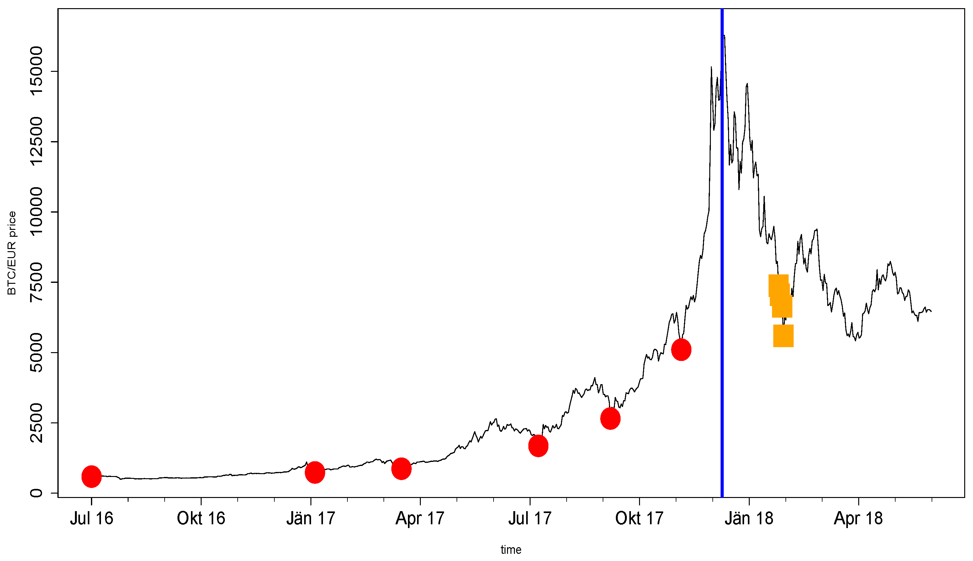Figure 2 shows the result for six Bitcoin momentum trades that are initiated after the halving event in 2016. The red points represent the entry dates: we chose entries on 9 July 2016 (directly at the halving event), 11 January 2017, 24 March 2017, 16 July 2017, 14 September 2017, and 12 November 2017. Note that all but the first entry date correspond to the troughs of major corrections. At this point, it is worth mentioning the high volatility of Bitcoin, since it establishes a harsh environment for the model to perform well. In other words, high noise variance results in high fluctuations around the mean of the asset price, which makes it hard for the model to detect the actual drift change point. Within the considered period, the drift change occurred at the local maximum on 16 December 2017 at EUR 16,590 per Bitcoin, designated by the blue vertical line in Figure 2. The model-implied optimal exit times are designated by the orange squares.

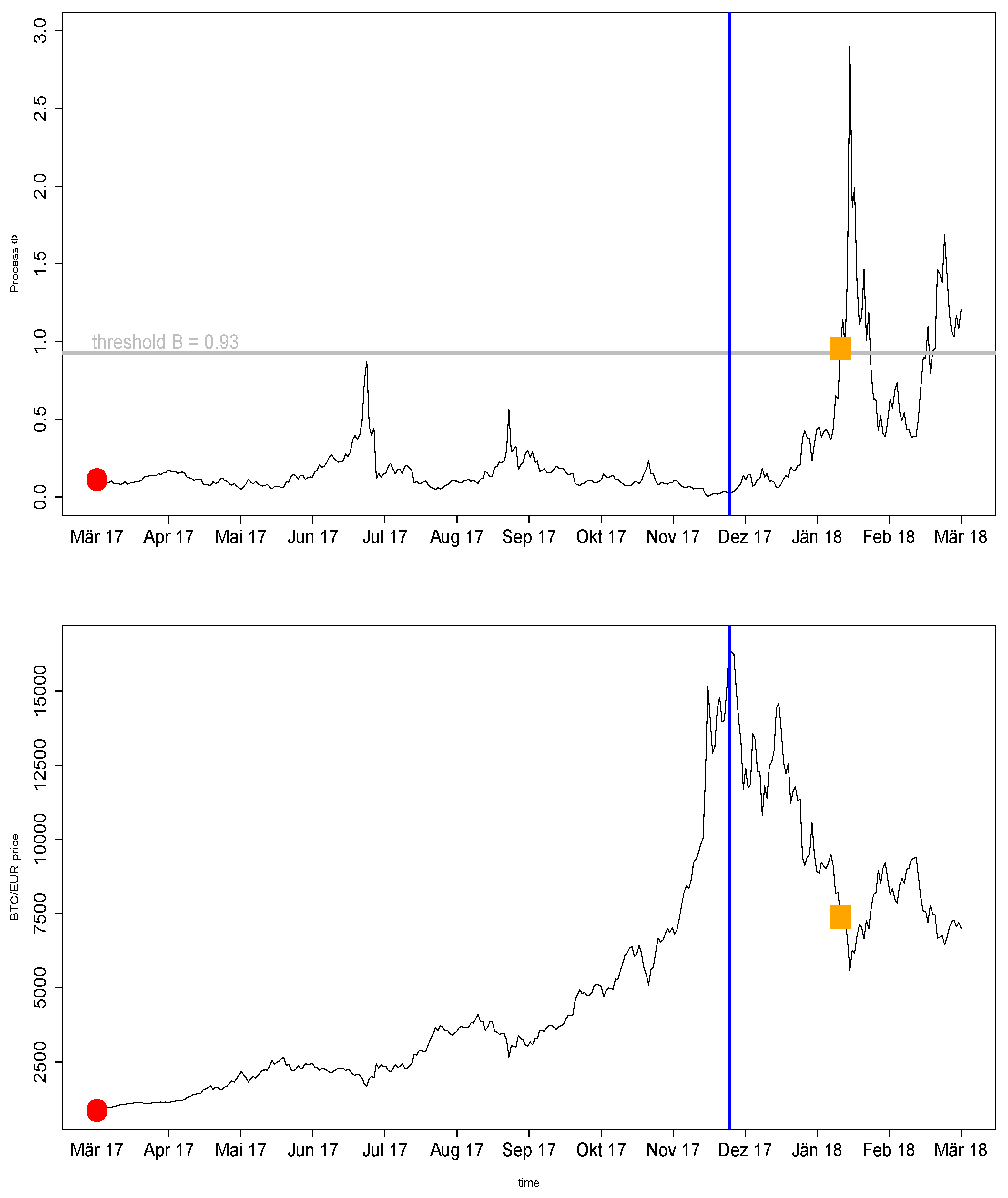
In Figure 3, we provide details on how the optimal exit time for the particular entry date, the March 2017 trade, is determined. We obtain the following parameter estimates of $\sigma =0.43$, ${\mu }_h=0.24$, ${\mu }_l=-0.49$, $\lambda =0.45$ and we fix $\alpha =-2$. Moreover, the solution of the free boundary equation is $B=0.93$. We initialize the process $\mathsf{\Phi }$ with ${\mathsf{\Phi }}_0=0.1$ (as for all other trades); hence, we set the probability of an immediate drift change after the entry to a pretty low value. The top pane represents $\mathsf{\Phi }$, and the lower pane represents the actual Bitcoin price after the entry of the long momentum trade on 24 March 2017, marked by the red point.

As is revealed in Figure 3, the correction in July 2017 almost triggered an exit, since the value of $\mathsf{\Phi }$ spiked rapidly, came very close to the barrier B. Although moving forward to the other major corrections in September 2017 and November 2017 also resulted in a spike, the levels reached are lower than the first one. Finally, when the Bitcoin price decreased significantly after the peak on 16 December 2017 marked by the vertical blue line, the optimal exit time was reached on 1 February 2018, when the probability ratio ${\mathsf{\Phi }}_t$ crossed the barrier B for the first time.

Returning to the analysis of the entire set of Bitcoin momentum trades again, the optimal exit times of July 2016, January 2017, and March 2017 trades are determined as 1 February 2018. The optimal exit time of the July 2017 trade is on 2 February 2018, of the September 2017 trade on 4 February 2018, and of the November 2017 trade on 5 February 2018. Thus, regardless of the dispersed entry dates, the corresponding optimal exit times are consolidated at the beginning of February 2018, more than a month after the local peak occurs. The returns of the respective trades heavily depend on the entry date, as an earlier entry results in a higher profit. Overall, returns spread between 1153%, corresponding to the July 2016 trade, and 9%, corresponding to the November 2017 trade. Note that these results are achieved using $\alpha =-2$.

Table 1. The table presents all key statistics corresponding to the six Bitcoin momentum trades that we introduced in the text. We estimated the parameters $\sigma$, ${\mu }_1$, ${\mu }_2$ and $\lambda$ based on Section 2.2. The column “Return” computes the return of the respective trades and the column “% of Maximum” is the performance measure to determine how much the exit price deviates from the peak of the Bitcoin bubble on 16 December 2017 (resp. on the exit date 29 April 2021).

$\mathit{\alpha }=-0.5$
Entry	$\mathbf{\sigma }$	${\mathbf{\mu }}_{\mathbf{2}}$	${\mathbf{\mu }}_{\mathbf{1}}$	$\mathbf{\lambda }$	B	Exit	Return	% of Maximum
2016-07-09	0.45	0.25	−0.12	0.45	1.90	2018-03-27	967.92%	37.92%
2017-01-11	0.43	0.24	−0.12	0.45	1.93	2018-03-29	690.01%	35.10%
2017-03-24	0.43	0.24	−0.12	0.45	1.93	2018-03-29	569.55%	35.10%
2017-07-16	0.42	0.27	−0.13	0.45	2.38	2018-03-30	232.98%	33.78%
2017-09-14	0.43	0.30	−0.15	0.45	3.11	2018-05-28	130.02%	36.81%
2017-11-12	0.43	0.33	−0.16	0.45	3.85	2018-06-10	13.05%	34.76%
$\mathbf{\alpha }=-\mathbf{1}$
Entry	$\mathbf{\sigma }$	${\mathbf{\mu }}_{\mathbf{2}}$	${\mathbf{\mu }}_{\mathbf{1}}$	$\mathbf{\lambda }$	B	Exit	Return	% of Maximum
2016-07-09	0.45	0.25	−0.25	0.45	1.27	2017-03-24	47.64%	5.24%
2017-01-11	0.43	0.24	−0.24	0.45	1.30	2018-02-05	658.49%	33.70%
2017-03-24	0.43	0.24	−0.24	0.45	1.30	2018-02-05	542.83%	33.70%
2017-07-16	0.42	0.27	−0.27	0.45	1.64	2018-02-05	232.19%	33.70%
2017-09-14	0.43	0.30	−0.30	0.45	2.20	2018-02-05	110.55%	33.70%
2017-11-12	0.43	0.33	−0.33	0.45	2.78	2018-03-29	14.14%	35.10%
$\mathbf{\alpha }=-\mathbf{2}$
Entry	$\mathbf{\sigma }$	${\mathbf{\mu }}_{\mathbf{2}}$	${\mathbf{\mu }}_{\mathbf{1}}$	$\mathbf{\lambda }$	B	Exit	Return	% of Maximum
2016-07-09	0.45	0.25	−0.49	0.45	0.89	2018-02-01	1153.49%	44.50%
2017-01-11	0.43	0.24	−0.49	0.45	0.92	2018-02-01	901.76%	44.50%
2017-03-24	0.43	0.24	−0.49	0.45	0.93	2018-02-01	749.01%	44.50%
2017-07-16	0.42	0.27	−0.54	0.45	1.23	2018-02-02	319.55%	42.56%
2017-09-14	0.43	0.30	−0.61	0.45	1.77	2018-02-04	150.18%	40.04%
2017-11-12	0.43	0.33	−0.66	0.45	2.36	2018-02-05	9.58%	33.70%
$\mathbf{\alpha }=-\mathbf{3}$
Entry	$\mathbf{\sigma }$	${\mathbf{\mu }}_{\mathbf{2}}$	${\mathbf{\mu }}_{\mathbf{1}}$	$\mathbf{\lambda }$	B	Exit	Return	% of Maximum
2016-07-09	0.45	0.25	−0.74	0.45	0.78	2017-07-15	195.92%	10.51%
2017-01-11	0.43	0.24	−0.73	0.45	0.82	2017-07-15	136.50%	10.51%
2017-03-24	0.43	0.24	−0.73	0.45	0.82	2017-07-15	100.43%	10.51%
2017-07-16	0.42	0.27	−0.81	0.45	1.15	2018-02-02	319.55%	42.56%
2017-09-14	0.43	0.30	−0.91	0.45	1.76	2018-02-04	150.18%	40.04%
2017-11-12	0.43	0.33	−0.98	0.45	2.45	2018-02-05	9.58%	33.70%
$\mathbf{\alpha }=-\mathbf{2}$
Entry	$\mathbf{\sigma }$	${\mathbf{\mu }}_{\mathbf{2}}$	${\mathbf{\mu }}_{\mathbf{1}}$	$\mathbf{\lambda }$	B	Exit	Return	% of Maximum
2020-10-16	0.43	0.26	−0.51	0.24	5.69	2021-04-29	356.18%	82.77%
2020-12-11	0.43	0.27	−0.54	0.24	9.53	2021-04-29	196.82 %	82.77%
2021-01-27	0.43	0.29	−0.57	0.24	61.89	2021-04-29	76.41%	82.77%

displays the results for all of the trades mentioned above using different values of $\alpha$. Altogether, all trades resulted in a positive return, regardless of the value of $\alpha$. Overall, $\alpha =-2$ yields the best performance, implying that Bitcoin price seems to fall faster in a bubble than it increases. This finding is in contrast with the result given in [9], which finds $\alpha =-1$ as the optimal parameter, implying that in a bubble, prices tend to increase and decrease at around the same speed among traditional asset classes.

Furthermore, we find that $\alpha =-0.5$ yields slightly better returns and performance than $\alpha =-1$. We attribute this result to the slower reaction of the model against the significant downturn in prices. To be precise, $\alpha =-0.5$ implies a higher value for the barrier B, which means that the value of ${\mathsf{\Phi }}_t$ should rise higher as well to trigger an exit. When we focus on the price of Bitcoin, we observe a major upward correction before the price heads down again. Thus, the first significant drop of more than 50% is ignored in the $\alpha =-0.5$ case, and consequently, the model suggests optimal exit times when the price started to free-fall again after a major upward correction.

Note that $\alpha =-3$ suggests optimal exit times earlier than the time point that the peak occurs, that is, the actual drift change point. One can explain this result by referring to the argument that we made above: As $\alpha =-3$ means that price decreases 3-times faster than it increases, on average, the model implies earlier optimal exit times compared to the cases with a lower value of $\alpha$. This fact is reflected in the result where the optimal exit time is found to be 15 July 2017. Actually, the major correction in July 2017 seems to be a volatility spike and not an actual drift change point, and accordingly, the model implied optimal exit time yields only 10.51% return. Overall, high volatility combined with a significant negative drift makes it hard for the model to perform well.

When we focus on the trades that are initiated after the halving event on 11 May 2020, we observe a significant decrease in the estimated value of $\lambda$. That, in turn, causes an increase in the boundary level B. Accordingly, the model does not suggest any exit within the given sample period. We instead assume an exit from the given long trades at the last date of the sample period.

Finally, we see that the return from an initiated Bitcoin momentum trade heavily depends on the entry date: the earlier we entered, the higher the expected return at the optimal exit time suggested by the model. This is because the model-implied optimal exit times are consolidated at the beginning of February, and an earlier entry means a lower entry price, at least in a bubble. Thus, based on our analysis, the model provides a supporting framework for exit decisions, but is by far not giving the magical formula to succeed in every trade.

4. Conclusions

In this paper, we investigate the performance of the partially observable digital-drift model of Ekström and Lindberg [6] and the corresponding optimal exit strategy on a Bitcoin trade. To estimate the unknown intensity of the random drift change time, we refer to Bitcoin halving events, which are critical events that push the price up eventually. Moreover, following [9], we suggest a drift parametrization that allows us to understand whether the Bitcoin prices fall faster than they rise or vice versa. Finally, after obtaining the in-sample parameter estimates, we run an out-of-sample performance test for the model.

The performance analysis of the model yields return values ranging between 9% and 1153%. We conclude that the return of the initiated Bitcoin momentum trades depends on the entry date: the earlier we entered, the higher the expected return at the optimal exit time suggested by the model. Moreover, our findings suggest that Bitcoin prices seem to fall faster in a bubble than they increase. Overall, to the extent of our analysis, the model provides a supporting framework for exit decisions, but is by far not the ultimate tool to succeed in every trade.