Abstract
In this paper, we consider numerical approximations of the Cahn–Hilliard type phase-field crystal model and construct a fully discrete finite element scheme for it. The scheme is the combination of the finite element method for spatial discretization and an invariant energy quadratization method for time marching. It is not only linear and second-order time-accurate, but also unconditionally energy-stable. We prove the unconditional energy stability rigorously and further carry out various numerical examples to demonstrate the stability and the accuracy of the developed scheme numerically.
Keywords:
phase-field crystal; IEQ; decoupled; linear; Cahn–Hilliard; unconditional energy stability MSC:
65N22; 65N12
1. Introduction
Crystallization is a phase change process involving mass transfer from liquid to solid. As a powerful modeling tool, the phase-field crystal model (PFC) has been used in this field to simulate the kinetics of atomic crystal growth in the crystallization process for more than two decades; see Elder et al. in [1,2]. The PFC model introduces a scalar function to represent the density of atoms. By assuming that the free energy contains a specific form of spatial gradient, and using the principle of variation to minimize the postulated total free energy, the governing equation can be derived naturally, and its solution is very similar to the periodic structure of the solid crystal lattice. The total free energy of the PFC model originally comes from the so-called Swift–Hohenberg (SH) model. The formats of the free energy of the two models are the same, but the way to derive the model is slightly different. The PFC model uses the so-called Cahn–Hilliard dynamics, and the latter SH model uses the so-called Allen–Cahn dynamics.
The purpose of this paper is to establish a completely discrete finite element algorithm for the classic PFC model. We expect that the designed scheme has the characteristics of linearity, second-order accuracy in time, and easy implementation. For the PFC model, many attempts have been made to achieve the numerical solution of various PFC models, such as the convex splitting method [3,4,5,6,7], invariant energy quadratic (IEQ) method [8,9,10,11], etc. Among them, the numerical schemes based on the convex splitting method have been established quite well, including the semi-discrete scheme in time, or the fully discrete scheme in space and time, as well as its energy stability and temporal and/or spatial error analysis. However, the nonlinear characteristics of the convex splitting method will cause a lot of computational cost in practical implementations. Therefore, in contrast, the linear algorithm appears to be more capable of saving calculation costs, such as the IEQ method. So far, however, the numerical scheme constructed by the IEQ method is only a semi-discrete format in time, that is, it is assumed that the space is continuous.
Therefore, this paper follows the idea of using the linearized IEQ method for time advancement in [8,9,10,11] and combines it with the spatial finite element method to obtain a fully discrete numerical scheme in time and space. Its main idea is to reconstruct the original system into an equivalent form by introducing an additional auxiliary variable. The design purpose of the new variable is to transform the nonlinear part of the energy density function into a quadratic function. The advantage of this method is that when the algorithm is designed, all nonlinear terms can be processed in a simple explicit–implicit combination manner. In this way, a linear finite element scheme with second-order accuracy in time can be easily obtained. Moreover, in the process of implementation, the auxiliary variable can help to split the original equation into two independent linear equations with constant coefficients, thereby greatly saving calculation costs.
The rest of the paper is organized as follows. In Section 2, we give a brief introduction to the PFC model. In Section 3, we develop a finite element numerical scheme and prove its unconditional stability. The detailed implementation process is also given. In Section 4, we present accuracy tests and numerous numerical examples to demonstrate the accuracy and efficiency of the developed scheme. Some concluding remarks are presented in Section 5.
2. Model and Its Energy Law
The PFC model was originally proposed in [12] to describe the phenomena of crystal growth on the atomic length and diffusive time scales. Its framework is to introduce a phase-field variable , where to represent the local density field of atoms, and t is the time.
The free energy of the PFC system is defined as follows
where is the Laplace operator, and is the nonlinear fourth-order polynomial potential. This free energy functional is the same as the Swift–Hohenburg energy; see also [1,2,13,14,15,16].
The dynamic equations can be derived as a gradient flow of the energy functional (1) in certain metrics. Taking the variational derivative of (1) in the negative norm gives the conservative Cahn–Hilliard type dynamic equations
where M is the mobility parameter, is the chemical potential that is derived by using , and .
3. Numerical Schemes
We now construct a fully discrete finite element numerical scheme for solving the PFC model (2) and (3). We focus on developing linear type schemes due to their easy-to-implement property. To this end, the main challenge lies in how to obtain a suitable time marching discretization approach for the nonlinear term . Different from the direct explicit or implicit discretization applied on it directly, we quadratize the nonlinear part of the energy density functional. We reformulate the total energy by introducing a new variable and then obtain a new system based on it. We must emphasize that the equivalent relationship between the final and the original system is the basic starting point.
We fix some notations here. Let be a time step size and set for . We denote by the inner product between functions and , and by the norm of the function .
3.1. Numerical Scheme
The free energy functional (1) is reformulated as
Note that a zero term is added in (6).
We define an auxiliary function as
where B is a positive constant. Since is a fourth-order polynomial term and it can always bound the quadratic term for any S, the integral term in (7) is bounded from below, and the constant B is used to ensure the radicand is further positive.
We further define another intermediate variable as
Using the variables , we obtain an equivalent PDE system as follows,
where
The initial conditions read as
The new system (9)–(12) still follows an energy dissipative law. By taking the inner product of (9) with , of (10) with , we derive
By taking the time derivative of (11), taking the inner product of the obtained equation with , and using integration by parts, we obtain
By multiplying (12) with , we have
Combining all equalities, we obtain the new energy dissipation law as follows,
where
Some finite dimensional discrete subspace is introduced as follows. Assuming that the polygonal/polyhedral domain is discretized by a conforming and shape regular triangulation/tetrahedron mesh that is composed by open disjoint elements K such that , we use to denote the space of polynomials of total degree at most l and define the following finite element spaces:
Hence,
We first formulate the PDE system (9)–(11) to the semi-discrete spatial discretization form, which reads as: find , such that
for .
Then, based on the second-order backward differentiation formula to discretize the time, and the finite element method for space, the second-order time-accurate finite element scheme for solving the system (22)–(25) is constructed as follows.
Assuming that and are known for , find , such that
for all , where
and is the second-order extrapolation for .
Remark 1.
The initialization of the second-order scheme (26)–(29) needs . These values can be obtained by constructing any type of first-order scheme. Moreover, we note that parameter S is adjustable in the definition of U in (7) from the fact that the fourth-order term in can always bound the negative quadratic term from below for any constant S. This means that the term in (27) acts as a stabilizer, which is used to balance the corresponding nonlinear term embedded in .
3.2. Energy Stability
Theorem 1.
3.3. Decoupled Implementation
The scheme (26)–(29) increases the number of the equations and forms a coupled system between the new variable U and the original variables . In principle, one expects to solve the decoupled system and avoid the computations of a large coupling system. By applying the nonlocal property of U, we can cause the system to be decoupled by the following process. Moreover, the existence and uniqueness of the scheme (26)–(29) is also shown in the following process.
First, we rewrite as the following linear combination form as
According to the nonlocal variable , the new system (41) can be split into two sub-systems, which read as
and
It is easy to solve the above two systems since they are linear and constant-coefficient.
A simple factorization for the above algebraic equation gives us
where
We show the solvability of (45) as follows. By setting , , , and combining the two obtained equations, we obtain
which implies . Therefore, (45) is always solvable.
Finally, we update , and by applying the linear splitting form (40), since , , , are obtained from (42) and (43), and is obtained from (45).
Therefore, we see that the extra auxiliary variable U will not cause extra computational cost. We do not need to solve the coupled system of equations even though the developed scheme (26)–(29) looks like a coupled system. Through this auxiliary variable, we can split the original scheme into three linear equations with constant coefficients that can be solved independently per time step. Therefore, the calculation cost of the entire scheme is only to solve the two linear systems (42) and (43).
Remark 2.
Concerning the existence and uniqueness of the scheme, we have shown it from the above implementation process. Using the splitting technique (40), we obtain (42) and (43). The existence and uniqueness of these two equations can be easily shown by using the Lax–Milgram theorem since these two equations are linear and every term is constant-coefficient. Moreover, (45) is also solvable since it is a simple linear algebraic equation, and , so is solvable.
4. Numerical Simulations
In this section, we will carry out several numerical examples to testify the accuracy of the proposed finite element scheme (26)–(29), which is denoted by FIEQ for short. In all examples, we use a 2D computational domain of and we adopt the FIEQ method to discretize the space where .
4.1. Accuracy Test
We now test the convergence rates of the FIEQ scheme. We set the 2D computational domain as and the order parameters as . We set the suitable forcing functions such that the exact solution of the system (2) and (3) is given by
To verify the temporal convergence order, we fix mesh size so that the grid size is sufficiently small and the spatial discretization errors are negligible compared with the time discretization error. In Figure 1a, we plot the errors of the phase variable between the numerical solution and the exact solution at with different time-step sizes. We observe that our proposed scheme presents perfect second-order convergence rates for the time step.
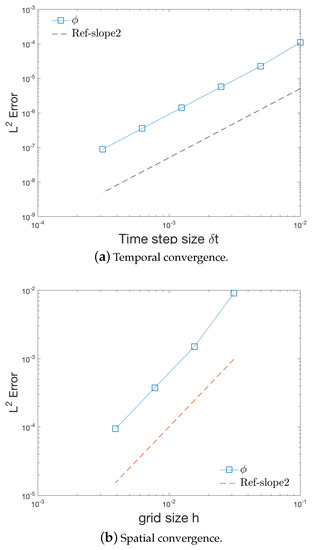
Figure 1.
(a) Convergence test in time where the numerical errors for the phase field variable are computed by using various time step size , and (b) convergence test in time where the numerical errors for the phase-field variable are computed by using various grid size h.
We continue to verify the accuracy of spatial convergence by applying the mesh refinement test for grid size h. In Figure 1b, we plot the errors of for various spatial grid size h. We choose sufficiently small () so that the errors are only dominated by the spatial discretization error. We use the numerical solutions obtained with a very tiny mesh size and computed by the scheme FIEQ as the exact solution approximately for computing errors. The error in the norm between the numerical solution and the exact solution at are plotted. We can see that the second-order convergence rates are followed by the -error of the phase-field variable , which are in agreement with the theoretical expectation of accuracy for element.
4.2. Phase Transition
In this example, the phase transition behavior of the PFC model is simulated. The similar numerical example can be found in [2,4,7,12,18,19]. With the computational domain of , the initial condition is set as , where is the random number in the range of . The Legendre polynomials of degrees up to 256 are used to discretize each direction. The order parameters are , . We use time step of to get the better accuracy. In Figure 2, we show the phase transition behavior of the density field at various times, and we can see that the profiles of random numbers finally grow to the crystals with BCC (body-centered-cubic) structure, which is similar to the results obtained in [2,4,7,12,18,19], qualitatively.
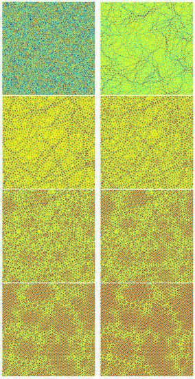
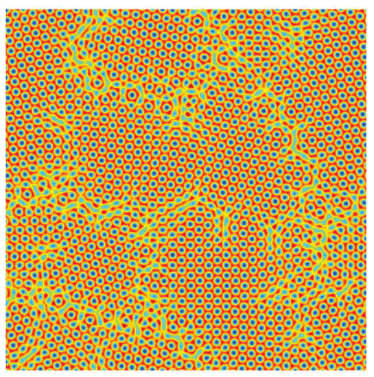
Figure 2.
The dynamical behaviors of the phase transition example, where snapshots of the numerical approximation of are taken at , 100, 250, 350, 500, 600, 750, 850, and 1000.
5. Concluding Remarks
We construct an effective fully discrete scheme for the phase-field crystal model based on finite element Galerkin scheme for spatial discretization. The scheme is also linear and unconditionally energy stable and has second-order accuracy in time, where the IEQ method is used for time discretization. The scheme is provably unconditionally energy-stable and very easy to implement. Through the implementations of several numerical examples, we demonstrate the accuracy and effectiveness of the developed scheme numerically. Moreover, the fully discrete scheme developed in this article is also applied for other types of gradient flow models to obtain the energy-stable and linear schemes.
Author Contributions
Data curation, J.Z.; Funding acquisition, J.Z.; Investigation, X.Y. All authors have read and agreed to the published version of the manuscript.
Funding
This research received no external funding.
Institutional Review Board Statement
Not applicable.
Informed Consent Statement
Not applicable.
Acknowledgments
This work is supported by University-level research fund project in Guizhou University of Finance and Economics (No. 2019XYB08), and Guizhou Key Laboratory of Big Data Statistics Analysis (No. BDSA20200102).
Conflicts of Interest
The authors declare no conflict of interest.
References
- Elder, K.R.; Grant, M. Modeling elastic and plastic deformations in nonequilibrium processing using phase field crystals. Phys. Rev. E 2004, 70, 051605. [Google Scholar] [CrossRef] [Green Version]
- Elder, K.R.; Katakowski, M.; Haataja, M.; Grant, M. Modeling elasticity in crystal growth. Phys. Rev. Lett. 2002, 88, 245701. [Google Scholar] [CrossRef] [PubMed] [Green Version]
- Eyre, D.J. Unconditionally gradient stable time marching the cahn- hilliard equation. In Computational and Mathematical Models of Microstruc- Tural Evolution; OPL: San Francisco, CA, USA, 1998; pp. 39–46. [Google Scholar]
- Feng, W.; Salgado, A.; Wang, C.; Wise, S.M. Preconditioned steepest descent methods for some nonlinear elliptic equations involving p-laplacian terms. J. Comput. Phys. 2017, 334, 45–67. [Google Scholar] [CrossRef] [Green Version]
- Wise, S.M.; Wang, C.; Lowengrub, J.S. An energy-stable and convergent finite-difference scheme for the phase field crystal equation. SIAM J. Numer. Anal. 2009, 47, 2269–2288. [Google Scholar] [CrossRef] [Green Version]
- Shen, J.; Wang, C.; Wang, S.; Wang, X. Second-order convex splitting schemes for gradient flows with Ehrlich-Schwoebel type energy: Application to thin film epitaxy. SIAM J. Numer. Anal. 2012, 50, 105–125. [Google Scholar] [CrossRef]
- Wang, C.; Wise, S.M. An energy stable and convergent finite-difference scheme for the modified phase field crystal equation. SIAM J. Numer. Anal. 2011, 49, 945–969. [Google Scholar] [CrossRef]
- Yang, X.; Han, D. Linearly first- and second-order, unconditionally energy stable schemes for the phase field crystal equation. J. Comput. Phys. 2017, 330, 1116–1134. [Google Scholar] [CrossRef] [Green Version]
- Zhang, J.; Yang, X. Efficient second order Unconditionally Stable time marching numerical scheme for a modified phase-field crystal model with a strong nonlinear vacancy potential. Comput. Phys. Commun. 2019, 245, 106860. [Google Scholar] [CrossRef]
- Zhang, J.; Yang, X. Numerical approximations for a new L2-gradient flow based Phase field crystal model with precise nonlocal mass conservation. Comput. Phys. Commun. 2019, 243, 51–67. [Google Scholar] [CrossRef]
- Zhang, J.; Yang, X. On Efficient numerical schemes for a two-mode phase field crystal model with face-centered-cubic (FCC) ordering structure. Appl. Numer. Math. 2019, 146, 13–37. [Google Scholar] [CrossRef]
- Wu, K.; Adland, A.; Karma, A. Phase-field-crystal model for fcc ordering. Phys. Rev. E 2010, 81, 061601. [Google Scholar] [CrossRef] [Green Version]
- Linhananta, A.; Sullivan, D.E. Mesomorphic polymorphism of binary mixtures of water and surfactants. Phys. Rev. E 1998, 57, 4547–4557. [Google Scholar] [CrossRef]
- Potemkin, I.I.; Panyukov, S.V. Microphase separation in correlated random copolymers: Mean-field theory and fluctuation corrections. Phys. Rev. E 1998, 57, 6902–6912. [Google Scholar] [CrossRef]
- Sagui, C.; Desai, R.C. Late-stage kinetics of systems with competing interactions quenched into the hexagonal phase. Phys. Rev. E 1995, 52, 2807–2821. [Google Scholar] [CrossRef]
- Swift, J.; Hohenberg, P.C. Hydrodynamic fluctuations at the convective instability. Phys. Rev. A 1977, 15, 319–328. [Google Scholar] [CrossRef] [Green Version]
- Gomez, H.; Nogueira, X. A new space-time discretization for the Swift-Hohenberg equation that strictly respects the Lyapunov functional. Commun. Nonlinear. Sci. Numer. Simulat. 2012, 17, 4930–4946. [Google Scholar] [CrossRef]
- Gomez, H.; Nogueira, X. An unconditionally energy-stable method for the phase field crystal equation. Comput. Methods Appl. Mech. Eng. 2012, 249–252, 52–61. [Google Scholar] [CrossRef]
- Hu, C.W.Z.; Wise, S.M.; Lowengrub, J.S. Stable and efficient finite difference nonlinear-multigrid schemes for the phase field crystal equation. J. Comput. Phys. 2009, 228, 5323–5339. [Google Scholar] [CrossRef] [Green Version]
Publisher’s Note: MDPI stays neutral with regard to jurisdictional claims in published maps and institutional affiliations. |
© 2022 by the authors. Licensee MDPI, Basel, Switzerland. This article is an open access article distributed under the terms and conditions of the Creative Commons Attribution (CC BY) license (https://creativecommons.org/licenses/by/4.0/).