Article

Approximations of Fuzzy Numbers by Using r-s Piecewise Linear Fuzzy Numbers Based on Weighted Metric

Institute of Operations Research and Cybernetics, Hangzhou Dianzi University, Hangzhou 310018, China
*
Author to whom correspondence should be addressed.
Mathematics 2022, 10(1), 145; https://doi.org/10.3390/math10010145
Submission received: 25 November 2021 / Revised: 26 December 2021 / Accepted: 29 December 2021 / Published: 4 January 2022
(This article belongs to the Section Fuzzy Sets, Systems and Decision Making)

Abstract

:
Using simple fuzzy numbers to approximate general fuzzy numbers is an important research aspect of fuzzy number theory and application. The existing results in this field are basically based on the unweighted metric to establish the best approximation method for solving general fuzzy numbers. In order to obtain more objective and reasonable best approximation, in this paper, we use the weighted distance as the evaluation standard to establish a method to solve the best approximation of general fuzzy numbers. Firstly, the conceptions of I-nearest r-s piecewise linear approximation (in short, PLA) and the II-nearest r-s piecewise linear approximation (in short, PLA) are introduced for a general fuzzy number. Then, most importantly, taking weighted metric as a criterion, we obtain a group of formulas to get the I-nearest r-s PLA and the II-nearest r-s PLA. Finally, we also present specific examples to show the effectiveness and usability of the methods proposed in this paper.

1. Introduction

Due to the complexity of the environment and the limitations of human inherent cognition, daily life is full of uncertain information. There are various approaches used to express and process this uncertain information, such as interval analysis [1,2], stochastic process [3] and fuzzy set theory [4]. In fuzzy set theory, a fuzzy number, which the notion was proposed by Zadeh in [5,6,7], has a good application in dealing with uncertain information. In recent years, a fuzzy number is very popular in the fields of cluster analysis, image recognition, system evaluation, automatic control, artificial intelligence and so on. Among them, multi-attribute decision making (MADM) with fuzzy information is the focus of scholars’ research [8,9].
In fact, when describing the characteristics of some fuzzy events, some fuzzy numbers are too complex. Therefore, the approximation of fuzzy numbers using regular fuzzy numbers to approximate complex fuzzy numbers has been deeply studied in fuzzy multi-attribute decision making. In the past few years, many scholars have obtained relevant important conclusions in this research field. For example, in [10], Ibrahim, Al-shami and Elbarbary defined the concept of (3,2)-fuzzy sets and establish the idea of relation in a (3,2)-fuzzy set and applied it to decision-making problems. In [11], with the aid of fuzzy soft β-neighborhoods, Atef, Ali and Al-shami introduced fuzzy soft covering-based multi-granulation fuzzy rough set models, which have a good application in solving multi-attribute group decision making (MAGDM) problems. In [12], Wang, Wan and Zhang further studied topological structures induced by L-fuzzifying approximation operators, where L denotes a completely distributive De Morgan algebra. In [13], Coroianu and Stefanini approximated fuzzy numbers by using the extended F-transform which always preserves the quasi-concavity property of a fuzzy number. In [14], by using the convolution method with useful properties for a general fuzzy number, Huang, Wu and Xie et al. constructed approximations comprising fuzzy number sequences. In [15], the approximation of fuzzy numbers by LR fuzzy numbers without constraints in the Euclidean class was studied by Yeh and Chu.
In addition, due to the simplification of calculation, data processing and management of uncertainty, the interval, triangular and trapezoidal approximation are very popularly studied and applied. In [16], Chanas proposed the notion of an approximation interval of a fuzzy number, and in [17,18], Grzegorzewski suggested two kinds of interval approximation operators successively to solve the problem of the interval approximation of fuzzy numbers. In [19], Ban and Coroianu found there exists at least a symmetric triangular fuzzy number which preserves a fixed parameter p P , which is a real parameter set related to fuzzy numbers. In [20], Abbasbandy and Hajjari suggested a weighted trapezoidal approximation of an arbitrary fuzzy number which preserves that the core is always a fuzzy number. In [21], Khastan and Moradi considered the width invariant trapezoidal and triangular approximations of fuzzy numbers, and its present methods avoid the effortful computation of Karush–Kuhn–Tucker theorem.
However, in some application situations, the trapezoidal approximation may be too restrictive and idealistic. Hence, in order to avoid the limitation of trapezoidal approximation and improve the accuracy, in [22], Coroianu, Gagolewski and Grzegorzewski defined the so-called piecewise linear 1-knot fuzzy numbers, which is simple enough and flexible to reconstruct the input fuzzy concepts, and further investigated some properties of the piecewise linear approximation of fuzzy numbers in [23]. Then, Wang and Shen proposed methods of approximating general fuzzy number by using a multi-knots piecewise linear fuzzy number in [24].
For a fuzzy number, it is known that the greater the value of the membership degree, the greater the contribution of the point to the fuzzy number, that is, the more important the point with the membership degree is. Therefore, compared with unweighted metric d ( u , v )   =   0 1 ( u ̲ ( r ) v ̲ ( r ) ) 2 d r + 0 1 ( u ¯ ( r ) v ¯ ( r ) ) 2 d r , weighted metric d * ( u , v )   =   0 1 2 r ( u ̲ ( r ) v ̲ ( r ) ) 2 d r + 0 1 2 r ( u ¯ ( r ) v ¯ ( r ) ) 2 d r is more reasonable and objective in describing the degree of difference between two fuzzy numbers.
In the study of approximating general fuzzy numbers with simple fuzzy numbers, for the convenience and simplicity of calculation, the methods established by predecessors (for example, see [22,23,24]) are basically based on unweighted metric. In order to establish a method to obtain a more objective and reasonable approximation solution, in this paper, we are going to use the weighted metric as the evaluation standard to explore the problem of using simple fuzzy numbers to approximate general fuzzy numbers. Of course, from the structure of the two metrics, the establishing of a method of solving the best approximation fuzzy numbers based on weighted metric is much more complex to calculate than that based on unweighted metric. This will bring some difficulties to the work we will do. However, from the structure of fuzzy numbers, the method we will establish will be able to obtain more reasonable and objective approximate solutions of general fuzzy numbers.
The specific arrangement of this paper is as follows: In Section 2, we briefly review some basic definitions, notations and results about fuzzy numbers. In Section 3, we give the conceptions of I-nearest r-s piecewise linear approximation and II-nearest r-s piecewise linear approximation for a general fuzzy number. Then, for a general fuzzy number, we obtain a group of calculation formulas of the I-nearest r-s piecewise linear approximation and the II-nearest r-s piecewise linear approximation. In Section 4, we give specific examples to show the effectiveness and usability of the methods in this paper, and compare some approximation methods of fuzzy numbers of the piecewise linear type. In Section 5, we make a brief summary to this paper and identify future research directions.

2. Basic Definitions and Notations

A fuzzy subset (in short, a fuzzy set) of the real line R is a function u : R [ 0 , 1 ] . For each such fuzzy set u, we denote by [ u ] r   =   { x R : u ( x ) r } for any r ( 0 , 1 ] , its r-level set. By supp u, we denote the support of u, i.e., the { x R : u ( x ) > 0 } . By [ u ] 0 , we denote the closure (according to the usual Euclidean topology on R) of the supp u, i.e., [ u ] 0   =   { x R : u ( x ) > 0 } ¯ .
If u is a normal and fuzzy convex fuzzy set of R, u ( x ) is upper semi-continuous, and [ u ] 0 is compact (according to the usual Euclidean topology on R), then we call u a fuzzy number, and denote the collection of all fuzzy numbers by E.
It is known that if u E , then for each r [ 0 , 1 ] , [ u ] r is a convex compact set in R, i.e., a closed interval. For u E , we denote the closed interval as [ u ] r   =   [ u ̲ ( r ) , u ¯ ( r ) ] for any r [ 0 , 1 ] .
For any u , v E , define u     v if and only if u ̲ ( r )     v ̲ ( r ) and u ¯ ( r )     v ¯ ( r ) for any r [ 0 , 1 ] .
The unweighted metric d on fuzzy numbers space E is defined [25] as
d ( u , v )   =   0 1 ( u ̲ ( r ) v ̲ ( r ) ) 2 d r + 0 1 ( u ¯ ( r ) v ¯ ( r ) ) 2 d r
for any u , v E .
The weighted metric d * on fuzzy numbers space E is defined [26] as
d * ( u , v )   =   0 1 2 r ( u ̲ ( r ) v ̲ ( r ) ) 2 d r + 0 1 2 r ( u ¯ ( r ) v ¯ ( r ) ) 2 d r
for any u , v E .
Let r   =   ( r 0 , r 1 , r 2 , , r m , r m + 1 ) , s   =   ( s 0 , s 1 , s 2 , , s n , s n + 1 ) with 0 =   r 0 < r 1 < r 2 < < r m < r m + 1   = 1 =   s n + 1 > s n > > s 2 > s 1 > s 0   = 0 . For any A   =   ( a 0 , a 1 , , a m + 1 ) and B   =   ( b 0 , b 1 , , b n + 1 ) with a 0     a 1     a 2     a m     a m + 1     b n + 1     b n   b 2     b 1     b 0 , then we call the fuzzy number u defined as
u ( x )   = 0 , x   <   a 0 r 1 x a 0 a 1 a 0 , x [ a 0 , a 1 ) r 1   +   ( r 2 r 1 ) x a 1 a 2 a 1 , x [ a 1 , a 2 ) r m 1   +   ( r m r m 1 ) x a m 1 a m a m 1 , x [ a m 1 , a m ) r m   +   ( 1 r m ) x a m a m + 1 a m , x [ a m , a m + 1 ) 1 , x [ a m + 1 , b n + 1 ] s n   +   ( 1 s n ) b n x b n b n + 1 , x ( b n + 1 , b n ] s n 1   +   ( s n s n 1 ) b n 1 x b n 1 b n , x ( b n , b n 1 ] s 1   +   ( s 2 s 1 ) b 1 x b 1 b 2 , x ( b 2 , b 1 ] s 1 b 0 x b 0 b 1 , x ( b 1 , b 0 ] 0 , x   >   b 0
is a r-s piecewise linear fuzzy number, and denote it as
u p l   =   P L ( A T , r T ; B T , s T )   =   P L a 0 r 0 a 1 r 1 a m r m a m + 1 r m + 1 ; b 0 s 0 b 1 s 1 b m s m b m + 1 s m + 1
and call r and s the left threshold value set and the right threshold value set of u p l , respectively. Specially, as r   =   s , we call the fuzzy number u p l a r-knots (i.e., r-knots) piecewise linear fuzzy number, and call r (i.e., s ) the threshold value set of u p l .
For example, as r   =   ( 0 , 0.3 , 0.6 , 0.9 , 1 ) , s = ( 0 , 0.2 , 0.5 , 0.8 , 1 ) , A   =   ( 1 , 0.7 , 0.6 , 0.2 , 0.1 ) and B   =   ( 1 , 0.6 , 0.4 , 0.1 , 0 ) , the membership function of u ˜   =   P L ( A T , r T ; B T , s T ) (see Figure 1), i.e.,
u ˜   =   P L 1 0 0.7 0.3 0.6 0.6 0.2 0.9 0.1 1 ; 1 0 0.6 0.2 0.4 0.5 0.1 0.8 0 1
is as follows:
u ˜ ( x )   = 0 , x   <   1 0.3 x ( 1 ) 0.7 ( 1 ) , x [ 1 , 0.7 ) 0.3   +   ( 0.6 0.3 ) x ( 0.7 ) 0.6 ( 0.7 ) , x [ 0.7 , 0.6 ) 0.6   +   ( 0.9 0.6 ) x ( 0.6 ) 0.2 ( 0.6 ) , x [ 0.6 , 0.2 ) 0.9   +   ( 1 0.9 ) x ( 0.2 ) 0.1 ( 0.2 ) , x [ 0.2 , 0.1 ) 1 , x [ 0.1 , 0 ] 0.8   +   ( 1 0.8 ) 0.1 x 0.1 0 , x ( 0 , 0.1 ] 0.5   +   ( 0.8 0.5 ) 0.4 x 0.4 0.1 , x ( 0.1 , 0.4 ] 0.2   +   ( 0.5 0.2 ) 0.6 x 0.6 0.4 , x ( 0.4 , 0.6 ] 0.2 1 x 1 0.6 , x ( 0.6 , 1 ] 0 , x   >   1
i.e.,
u ˜ ( x )   = 0 , x   <   1 x   +   1 , x [ 1 , 0.7 ) 3 x   +   2.4 , x [ 0.7 , 0.6 ) 0.75 x   +   1.05 , x [ 0.6 , 0.2 ) x   +   1.1 , x [ 0.2 , 0.1 ) 1 , x [ 0.1 , 0 ] 1     x , x ( 0 , 0.1 ] 0.9     x , x ( 0.1 , 0.4 ] 1.1     x , x ( 0.4 , 0.6 ] 1 x 2 , x ( 0.6 , 1 ] 0 , x   >   1
For fixed r i , s j [ 0 , 1 ] with 0 =   r 0 < r 1 < r 2 < < r m < r m + 1   = 1 =   s n + 1 > s n > > s 2 > s 1 > s 0   = 0 , we denote the collection r-s piecewise linear fuzzy numbers by r P L s ( E ) , and denote the collection of all r-knots (s-knots) piecewise linear fuzzy numbers by P L r ( E ) (i.e., P L s ( E ) ).
Let u   =   u p l r P L s ( E ) . Then,
u ̲ ( r )   = a 0   +   ( a 1 a 0 ) r r 1 , r [ r 0 , r 1 ] = [ 0 , r 1 ] a 1   +   ( a 2 a 1 ) r r 1 r 2 r 1 , r ( r 1 , r 2 ] a m 1   +   ( a m a m 1 ) r r m 1 r m r m 1 , r ( r m 1 , r m ] a m   +   ( a m + 1 a m ) r r m 1 r m , r ( r m , r m + 1 ] = ( r m , 1 ]
and
u ¯ ( r )   = b 0   +   ( b 1 b 0 ) r s 1 , r [ s 0 , s 1 ] = [ 0 , s 1 ] b 1   +   ( b 2 b 1 ) r s 1 s 2 s 1 , r ( s 1 , s 2 ] b n 1   +   ( b n b n 1 ) r s n 1 s n s n 1 , r ( s n 1 , s n ] b n   +   ( b n + 1 b n ) r s n 1 s n , r ( s n , s n + 1 ] = ( s n , 1 ]
for r [ 0 , 1 ] .
Let R n × n be the collection of all n   ×   n real matrices (i.e., the matrices with all real number elements). If matrix A   =   ( a i j ) n × n R n × n satisfies
| a i i |   >   j = 1 , j i n | a i j | ,   i   =   1 ,   2 ,   ,   n
then A is a strictly diagonally dominant matrix (see Theorem I in [27]).
If A   =   ( a i j ) n × n R n × n is a strictly diagonally dominant matrix with positive diagonal entries (i.e., a i i   >   0 , i   =   1 ,   2 ,   ,   n ), then
λ i   >   0
for any i   =   1 ,   2 ,   ,   n , where λ i ( i = 1 , 2 , , n ) is the eigenvalues of A (see Theorem VII in [27]).

3. The Approximations of Membership Functions

In [18], Coroianu, Gagolewski and Grzegorzewski give a method of approximating general fuzzy numbers by using piecewise linear 1-knot fuzzy numbers with respect to the metric d. In this section, we are going to establish a recursion formula to obtain the r-s piecewise linear fuzzy number which is the nearest (with respect to metric d * ) approximation with the left threshold value set r and the right threshold value set s . To do this, we first give the following definitions and theorems.
Definition 1.
Let r i , s j [ 0 , 1 ] with 0 =   r 0 < r 1 < r 2 < < r m < r m + 1   = 1 =   s n + 1 > s n > > s 2 > s 1 > s 0   = 0 . If there exists u p l r P L s ( E ) with u p l ̲ ( 0 )   =   u ̲ ( 0 ) , u p l ¯ ( 0 )   =   u ¯ ( 0 ) , u p l ̲ ( 1 )   =   u ̲ ( 1 ) , u p l ¯ ( 1 )   =   u ¯ ( 1 ) (i.e., [ u p l ] 0   =   [ u ] 0 and [ u p l ] 1   =   [ u ] 1 ) such that
d * ( u , u p l )   =   min { d * ( u , v ) : v r P L s ( E ) with [ v ] 0   =   [ u ] 0 , [ v ] 1   =   [ u ] 1 }
then we say u p l to be the I-nearest (with respect to metric d * ) r-s piecewise linear approximation (in short, PLA) of fuzzy number u. Specially, as r   =   s , we say u p l to be the I-nearest (with respect to metric d * ) r-knots (i.e., s-knots) piecewise linear approximation (in short, PLA) of fuzzy number u.
Definition 2.
Let r i , s j [ 0 , 1 ] with 0 =   r 0 < r 1 < r 2 < < r m < r m + 1   = 1 =   s n + 1 > s n > > s 2 > s 1 > s 0   = 0 . If there exists u p l r P L s ( E ) such that
d * ( u , u p l )   =   min { d * ( u , v ) : v r P L s ( E ) }
then we say u p l to be the II-nearest (with respect to metric d * ) r-s piecewise linear approximation (in short, PLA) of fuzzy number u. Specially, as r   =   s , we say u p l to be the II-nearest (with respect to metric d * ) r-knots (i.e., s-knots) piecewise linear approximation (in short, PLA) of fuzzy number u.
By the definitions of the I-nearest (with respect to metric d * ) r-s piecewise linear approximation and the II-nearest (with respect to metric d * ) r-s piecewise linear approximation of a fuzzy number, we can directly get the following result:
Proposition 1.
Let u E and r i , s j [ 0 , 1 ] with 0   =   r 0 < r 1 < r 2 < < r m < r m + 1   = 1   =   s n + 1 > s n > > s 2 > s 1 > s 0   = 0 to be the I-nearest (with respect to metric d * ) r-s piecewise linear approximation of fuzzy number u, and v p l to be the II-nearest (with respect to metric d * ) r-s piecewise linear approximation of fuzzy number u. Then,
d * ( u , v p l )     d * ( u , u p l )
i.e., v p l is a better approximation of fuzzy number u than u p l .
Proof. 
From
{ d * ( u , v ) : v r P L s ( E ) with [ v ] 0   =   [ u ] 0 , [ v ] 1   =   [ u ] 1 } { d * ( u , v ) : v r P L s ( E ) }
We see that
d * ( u , u p l ) = min { d * ( u , v ) : v r P L s ( E ) with [ v ] 0   =   [ u ] 0 , [ v ] 1   =   [ u ] 1 } min { d * ( u , v ) : v r P L s ( E ) } =   d * ( u , v p l )
The proof of the proposition can be completed. □
For convenience, we give the following notations:
Let r   =   ( r 0 , r 1 , r 2 , , r m , r m + 1 ) , s   =   ( s 0 , s 1 , s 2 , , s n , s n + 1 ) with 0 =   r 0 < r 1 < r 2 < < r m < r m + 1   = 1 =   s n + 1 > s n > > s 2 > s 1 > s 0   = 0 . We give the following notations:
α i ̲   = Δ r 2 2 Σ r 2 2 Σ r 1 2 , i   =   1 Δ r i + 1 2 Σ r i + 1 2 Σ r i 2 Δ r i 2 α i 1 ̲ , i   =   2   , 3   ,   ,   m 1
β i ̲   = γ 1 ̲ + λ 1 ̲ r 1 2 u ̲ ( 0 ) Σ r 2 2 Σ r 1 2 , i   =   1 γ i ̲ + λ i ̲ Δ r i 2 β i 1 ̲ Σ r i + 1 2 Σ r i 2 Δ r i 2 α i 1 ̲ , i   =   2   , 3   ,   ,   m 1
where, Σ r i   =   r i   +   r i 1 , Δ r i 2   =   r i 2     r i 1 2 , γ i ̲   =   12 r i r i 1 r i 1 r i u ̲ ( r ) ( r r i 1 ) r d r and λ i ̲   =   12 r i + 1 r i r i r i + 1 u ̲ ( r ) ( r i + 1 r ) r d r .
α j ¯   = Δ s 2 2 Σ s 2 2 Σ s 1 2 , j   =   1 Δ s j + 1 2 Σ s j + 1 2 Σ s j 2 Δ s j 2 α j 1 ¯ , j   =   2   , 3   ,   ,   n 1
β j ¯   = γ 1 ¯ + λ 1 ¯ s 1 2 u ¯ ( 0 ) Σ s 2 2 Σ s 1 2 , j   =   1 γ j ¯ + λ j ¯ Δ s j 2 β j 1 ¯ Σ s j + 1 2 Σ s j 2 Δ s j 2 α j 1 ¯ , j   =   2   , 3   ,   ,   n 1
where, Σ s j   =   s j   +   s j 1 , Δ s j 2   =   s j 2 s j 1 2 , γ j ¯   =   12 s j s j 1 s j 1 s j u ¯ ( r ) ( r s j 1 ) r d r and λ j ¯   =   12 s j + 1 s j s j s j + 1 u ¯ ( r ) ( s j + 1 r ) r d r .
Theorem 1.
Let r   =   ( r 0 , r 1 , r 2 , , r m , r m + 1 ) , s   =   ( s 0 , s 1 , s 2 , , s n , s n + 1 ) with 0 =   r 0 < r 1 < r 2 < < r m < r m + 1   = 1 =   s n + 1 > s n > > s 2 > s 1 > s 0   = 0 . If a i , b j R ( i = 1 , 2 , , m , j = 1 , 2 , , n ) are respectively determined by following recursion formulas:
a m   =   γ m ̲ + λ m ̲ ( 1 r m 2 ) u ̲ ( 1 ) Δ r m 2 β m 1 ̲ Σ r m + 1 2 Σ r m 2 Δ r m 2 α m 1 ̲ a i   =   β i ̲ α i ̲ · a i + 1 ,   i   =   m 1 ,   m 2   ,   ,   1
and
b n   =   γ n ¯ + λ n ¯ ( 1 s n 2 ) u ¯ ( 1 ) Δ s n 2 β n 1 ¯ Σ s n + 1 2 Σ s n 2 Δ s n 2 α n 1 ¯ b j   =   β j ¯ α j ¯ · b j + 1 ,   j   =   n 1 ,   n 2 ,   ,   1
and satisfy u ̲ ( 0 ) =   a 0 a 1 a 2 a m a m + 1   = u ̲ ( 1 ) u ¯ ( 1 ) =   b n + 1 b n b 2 b 1 b 0   = u ¯ ( 0 ) , then
u p l   =   P L ( A T , r T ; B T , s T )   =   P L a 0 r 0 a 1 r 1 a m r m a m + 1 r m + 1 , b 0 s 0 b 1 s 1 b m s m b m + 1 s m + 1
is the I-nearest (with respect to metric d * ) r-s piecewise linear approximation of fuzzy number u, where A   =   ( a 0 , a 1 , a m + 1 )   =   ( u ̲ ( 0 ) , a 1 , , u ̲ ( 1 ) ) and B   =   ( b 0 , b 1 , b n + 1 )   =   ( u ¯ ( 0 ) , b 1 , , u ¯ ( 1 ) ) , and α i ̲ , β i ̲ , α j ¯ , β j ¯ ( i   =   1 , 2 , , m , j   =   1 , 2 , , n ) are respectively determined by Formulas (7)–(10).
Proof. 
We denote the n-dimensional Euclidean space as R n for positive integer n. For any x   =   ( x 1 , , x m ) R m , y   =   ( y 1 , , y n ) R n with x 1     x 2     x m     y n   y 2     y 1 , we denote X   =   ( u ̲ ( 0 ) , x 1 , x 2 , , x m , u ̲ ( 1 ) ) ,   Y   =   ( u ¯ ( 0 ) , y 1 , y 2 , , y n , u ¯ ( 1 ) ) and u x , y   =   P L ( X , r ; Y , s ) .
We define D : R m + n R as
D ( x 1 , x 2 , , x m , y 1 , y 2 , , y n )   =   D ( x , y )   =   ( d * ( u , u x , y ) ) 2
for any ( x , y )   =   ( x 1 , x 2 , , x m , y 1 , y 2 , , y n ) R m + n . By the definition of weighted metric d * (i.e, Equation (2)), we see that
D ( x 1 , x 2 , , x m , y 1 , y 2 , , y n )   =   0 1 2 r ( u ̲ ( r ) u x , y ̲ ( r ) ) 2 d r   +   0 1 2 r ( u ¯ ( r ) u x , y ¯ ( r ) ) 2 d r
By the definition of u ̲ ( r ) and u ¯ ( r ) (see Formulas (5) and (6)), let r 0   =   0 ,   r m + 1   =   1 ,   x 0   =   u ̲ ( 0 ) ,   x m + 1   =   u ̲ ( 1 ) ,   s 0   =   0 ,   s n + 1 = 1 ,   y 0   =   u ¯ ( 0 ) and y n + 1   =   u ¯ ( 1 ) , we have that
0 1 2 r ( u ̲ ( r ) u x , y ̲ ( r ) ) 2 d r = 0 r 1 2 r ( u ̲ ( r ) u ̲ ( 0 ) ( x 1 u ̲ ( 0 ) ) r r 1 ) 2 d r   +   r 1 r 2 2 r ( u ̲ ( r ) x 1 ( x 2 x 1 ) r r 1 r 2 r 1 ) 2 d r +   k = 2 i 2 r k r k + 1 2 r ( u ̲ ( r ) x k ( x k + 1 x k ) r r k r k + 1 r k ) 2 d r + r i 1 r i 2 r ( u ̲ ( r ) x i 1 ( x i x i 1 ) r r i 1 r i r i 1 ) 2 d r + r i r i + 1 2 r ( u ̲ ( r ) x i ( x i + 1 x i ) r r i r i + 1 r i ) 2 d r +   k = i + 1 m 2 r k r k + 1 2 r ( u ̲ ( r ) x k ( x k + 1 x k ) r r k r k + 1 r k ) 2 d r + r m 1 r m 2 r ( u ̲ ( r ) x m 1 ( x m x m 1 ) r r m 1 r m r m 1 ) 2 d r + r m 1 2 r ( u ̲ ( r ) x m ( u ̲ ( 1 ) x m ) r r m 1 r m ) 2 d r
and
0 1 2 r ( u ¯ ( r ) u x , y ¯ ( r ) ) 2 d r = 0 s 1 2 r ( u ¯ ( r ) u ¯ ( 0 ) ( y 1 u ¯ ( 0 ) ) r s 1 ) 2 d r   +   s 1 s 2 2 r ( u ¯ ( r ) y 1 ( y 2 y 1 ) r s 1 s 2 s 1 ) 2 d r + k = 2 j 2 s k s k + 1 2 r ( u ¯ ( r ) y k ( y k + 1 y k ) r s k s k + 1 s k ) 2 d r + s j 1 s j 2 r ( u ¯ ( r ) y j 1 ( y j y j 1 ) r s j 1 s j s j 1 ) 2 d r + s j s j + 1 2 r ( u ¯ ( r ) y j ( y j + 1 y j ) r s j s j + 1 s j ) 2 d r +   k = j + 1 n 2 s k s k + 1 2 r ( u ¯ ( r ) y k ( y k + 1 y k ) r s k s k + 1 s k ) 2 d r + s n 1 s n 2 r ( u ¯ ( r ) y n 1 ( y n y n 1 ) r s n 1 s n s n 1 ) 2 d r + s n 1 2 r ( u ¯ ( r ) y n ( u ¯ ( 1 ) y n ) r s n 1 s n ) 2 d r
Then, for any fixed i   =   1   ,   2   ,   ,   m , we have that
D ( x 1 , x 2 , , x m , y 1 , y 2 , , y n ) x i = x i [ r i 1 r i 2 r ( u ̲ ( r ) x i 1 ( x i x i 1 r r i 1 r i r i 1 ) 2 ) d r + r i r i + 1 2 r ( u ̲ ( r ) x i ( x i + 1 x i r r i r i + 1 r i ) 2 ) d r ] = x i [ x i 2 ( r i r i 1 ) 2 r i 1 r i 2 r ( r r i 1 ) 2 d r 2 x i r i r i 1 r i 1 r i 2 r ( r r i 1 ) ( u ̲ ( r ) x i 1 r i r r i r i 1 ) d r + r i 1 r i 2 r ( u ̲ ( r ) x i 1 r i r r i r i 1 ) 2 d r   +   x i 2 ( r i + 1 r i ) 2 r i r i + 1 2 r ( r i + 1 r ) 2 d r 2 x i r i + 1 r i r i r i + 1 2 r ( r i + 1 r ) ( u ̲ ( r ) x i + 1 r r i r i + 1 r i ) d r + r i r i + 1 2 r ( u ̲ ( r ) x i + 1 r r i r i + 1 r i ) 2 d r ] = 4 x i ( r i r i 1 ) 2 r i 1 r i r ( r r i 1 ) 2 d r 4 r i r i 1 r i 1 r i r ( r r i 1 ) ( u ̲ ( r ) x i 1 r i r r i r i 1 ) d r + 4 x i ( r i + 1 r i ) 2 r i r i + 1 r ( r i + 1 r ) 2 d r 4 r i + 1 r i r i r i + 1 r ( r i + 1 r ) ( u ̲ ( r ) x i + 1 r r i r i + 1 r i ) d r = 1 3 ( r i 2 r i 1 2 ) x i 1   +   1 3 ( ( r i + 1 + r i ) 2 ( r i + r i 1 ) 2 ) x i   +   1 3 ( r i + 1 2 r i 2 ) x i + 1 4 r i r i 1 r i 1 r i u ̲ ( r ) ( r r i 1 ) r d r 4 r i + 1 r i r i r i + 1 u ̲ ( r ) ( r i + 1 r ) r d r
Likewise, for any fixed j   =   1 ,   2 ,   ,   n , we have that
D ( x 1 , x 2 , , x m , y 1 , y 2 , , y n ) y j = y j [ s j 1 s j 2 r ( u ¯ ( r ) y j 1 ( y j y j 1 r s j 1 s j s j 1 ) 2 ) d r + s j s j + 1 2 r ( u ¯ ( r ) y j ( y j + 1 y j r s j s j + 1 s j ) 2 ) d r ] = y j [ y j 2 ( s j s j 1 ) 2 s j 1 s j 2 r ( r s j 1 ) 2 d r 2 y j s j s j 1 s j 1 s j 2 r ( r s j 1 ) ( u ¯ ( r ) y j 1 s j r s j s j 1 ) d r + s j 1 s j 2 r ( u ¯ ( r ) y j 1 s j r s j s j 1 ) 2 d r + y j 2 ( s j + 1 s j ) 2 s j s j + 1 2 r ( s j + 1 r ) 2 d r 2 y j s j + 1 s j s j s j + 1 2 r ( s j + 1 r ) ( u ¯ ( r ) y j + 1 r s j s j + 1 s j ) d r + s j s j + 1 2 r ( u ¯ ( r ) y j + 1 r s j s j + 1 s j ) 2 d r ] = 4 y j ( s j s j 1 ) 2 s j 1 s j r ( r s j 1 ) 2 d r 4 s j s j 1 s j 1 s j r ( r s j 1 ) ( u ¯ ( r ) y j 1 s j r s j s j 1 ) d r + 4 y j ( s j + 1 s j ) 2 s j s j + 1 r ( s j + 1 r ) 2 d r 4 s j + 1 s j s j s j + 1 r ( s j + 1 r ) ( u ¯ ( r ) y j + 1 r s j s j + 1 s j ) d r = 1 3 ( s j 2 s j 1 2 ) y j 1 + 1 3 ( ( s j + 1 + s j ) 2 ( s j + s j 1 ) 2 ) y j + 1 3 ( s j + 1 2 s j 2 ) y j + 1 4 s j s j 1 s j 1 s j u ¯ ( r ) ( r s j 1 ) r d r 4 s j + 1 s j s j s j + 1 u ¯ ( r ) ( s j + 1 r ) r d r
Let
D ( x 1 , x 2 , , x m , y 1 , y 2 , , y n ) x i   =   0 ,   i   =   1 ,   2 ,   ,   m
and
D ( x 1 , x 2 , , x m , y 1 , y 2 , , y n ) y j   =   0 ,   j   =   1 ,   2 ,   ,   n
Then, we can obtain that
C 1 x T   = γ 1 ̲ + λ 1 ̲ r 1 2 u ̲ ( 0 ) γ 2 ̲ + λ 2 ̲ γ i ̲ + λ i ̲ γ m ̲ + λ m ̲ ( 1 r m 2 ) u ̲ ( 1 )
and
C 2 y T   = γ 1 ¯ + λ 1 ¯ r 1 2 u ¯ ( 0 ) γ 2 ¯ + λ 2 ¯ γ j ¯ + λ j ¯ γ n ¯ + λ n ¯ ( 1 s n 2 ) u ¯ ( 1 )
where, x T is the transposition of x   =   ( x 1 , x 2 , x m ) , y T is the transposition of y   =   ( y 1 , y 2 , y n ) , and
C 1   = Σ r 2 2 Σ r 1 2 Δ r 2 2 0 0 0 0 Δ r 2 2 Σ r 3 2 Σ r 2 2 Δ r 3 2 0 0 0 0 0 0 Δ r m 1 2 Σ r m 2 Σ r m 1 2 Δ r m 2 0 0 0 0 Δ r m 2 Σ r m + 1 2 Σ r m 2
and
C 2   = Σ s 2 2 Σ s 1 2 Δ s 2 2 0 0 0 0 Δ s 2 2 Σ s 3 2 Σ s 2 2 Δ s 3 2 0 0 0 0 0 0 Δ s n 1 2 Σ s n 2 Σ s n 1 2 Δ s n 2 0 0 0 0 Δ s n 2 Σ s n + 1 2 Σ s n 2
From 0   =   r 0 < r 1 < r 2 < < r m < r m + 1   =   1 =   s n + 1 > s n > > s 2 > s 1 > s 0   = 0 , we see that Δ r i + 1 2   >   0   , i   =   1 ,   2 ,   ,   m and Δ s j + 1 2   >   0 ,   j   =   1 ,   2 ,   ,   n , so
| Σ r 2 2 Σ r 1 2 |   >   | Δ r 2 2 | | Σ r i + 1 2 Σ r i 2 |   >   | Δ r i 2 | + | Δ r i + 1 2 | ,   i   =   2 ,   3 ,   ,   m 1 | Σ r m + 1 2 Σ r m 2 |   >   | Δ r m 2 |
and
| Σ s 2 2 Σ s 1 2 |   >   | Δ s 2 2 | | Σ s j + 1 2 Σ s j 2 |   >   | Δ s j 2 | + | Δ s j + 1 2 | , i   =   2 ,   3 ,   ,   n 1 | Σ s n + 1 2 Σ s n 2 |   >   | Δ s n 2 |
Therefore, C 1 and C 2 are both a strictly diagonally dominant matrix. Thus, by Thomas algorithm in [27], we know that there is a unique set of solutions for the two equations for linear Equation (13) of unknown quantities x 1 , x 2 , x m and linear Equation (14) of unknown quantities y 1 , y 2 , y n (denote the solutions set of (13) as ( a 1 , a 2 , , a m ) and the solutions set of (14) as ( b 1 , b 2 , , b n ) ), and the solutions sets ( a 1 , a 2 , , a m ) and ( b 1 , b 2 , , b n ) are determined by recursion formulas (11) and (12).
Denoting A =   ( a 0 , a 1 , a 2 , , a m , a m + 1 )   =   ( u ̲ ( 0 ) , a 1 , a 2 , , a m , u ̲ ( 1 ) ) ,   B =   ( b 0 , b 1 , b 2 , , b n , b n + 1 )   =   ( u ¯ ( 0 ) , b 1 , b 2 , , b n , u ¯ ( 1 ) ) , by u ̲ ( 0 ) =   a 0 a 1 a 2 a m a m + 1   = u ̲ ( 1 ) u ¯ ( 1 ) =   b n + 1 b n b 2 b 1 b 0   = u ¯ ( 0 ) , we can define the r-s piecewise linear fuzzy number as u p l   =   P L ( A T , r T ; B T , s T ).
In the following, in order to show that the r-s piecewise linear fuzzy number u p l is the I-nearest (with respect to metric d * ) r-s piecewise linear approximation of fuzzy number u, we only show that the Hessian matrix of the function D ( x 1 , x 2 , , x m , y 1 , y 2 , , y n ) of m   +   n variables is a positive definite matrix as ( x 1 , x 2 , , x m , y 1 , y 2 , , y n ) = ( a 1 , a 2 , , a m , b 1 , b 2 , , b n ) .
From the expressions of D ( x 1 , x 2 , , x m , y 1 , y 2 , , y n ) x i ( i   =   1 ,   2 ,   ,   m ) , which we obtained before, we have that
D ( x 1 , x 2 , , x m , y 1 , y 2 , , y n ) x 1 x k = 1 3 ( Σ r 2 2 Σ r 1 2 ) , k   =   1 1 3 Δ r 2 2 , k   =   2 0 , k   =   3 ,   4 ,   ,   m
D ( x 1 , x 2 , , x m , y 1 , y 2 , , y n ) x i x k = 1 3 Δ r i 2 , k   =   i 1 1 3 ( Σ r i + 1 2 Σ r i 2 ) , k   =   i 1 3 Δ r i + 1 2 , k = i + 1 0 , k   =   1 ,   2 ,   ,   i 2 ,   i + 2 ,   ,   m
for i   =   2 ,   3 ,   ,   m 1 , and
D ( x 1 , x 2 , , x m , y 1 , y 2 , , y n ) x m x k   = 1 3 Δ r m 2 , k   =   m 1 1 3 ( Σ r m + 1 2 Σ r m 2 ) , k   =   m 0 , k   =   1 ,   2 ,   ,   m 2
From the expressions of D ( x 1 , x 2 , , x m , y 1 , y 2 , , y n ) y j ( j   =   1 ,   2 ,   ,   n ) , which we obtained before, we have that
D ( x 1 , x 2 , , x m , y 1 , y 2 , , y n ) y 1 y k   = 1 3 ( Σ s 2 2 Σ s 1 2 ) , k   =   1 1 3 Δ s 2 2 , k   =   2 0 , k   =   3 ,   4 ,   ,   n
D ( x 1 , x 2 , , x m , y 1 , y 2 , , y n ) y j y k   = 1 3 Δ s j 2 , k   =   j 1 1 3 ( Σ s j + 1 2 Σ s j 2 ) , k   =   j 1 3 Δ s j + 1 2 , k   =   j + 1 0 , k   =   1 ,   2 ,   ,   j 2 ,   j + 2 ,   ,   n
for j   =   2 ,   3 ,   ,   n 1 , and
D ( x 1 , x 2 , , x m , y 1 , y 2 , , y n ) y n y k   = 1 3 Δ s n 2 , k   =   n 1 1 3 ( Σ s n + 1 2 Σ s n 2 ) , k   =   n 0 , k   =   1 ,   2 ,   , n 2
Therefore, we can obtain the Hessian matrix of the function D ( x 1 , x 2 , , x m , y 1 , y 2 , , y n ) at ( a 1 , a 2 , , a m , b 1 , b 2 , , b n ) as follow:
C   =   1 3 C 1 0 0 C 2
Since C 1 and C 2 are all strictly diagonally dominant and real symmetric, C is strictly diagonally dominant and real symmetric. It implies that the eigenvalues of C are all positive values, so C is a positive matrix. Therefore, ( a 1 , a 2 , , a m , b 1 , b 2 , , b n ) is the minimum point of D ( x 1 , x 2 , , x m , y 1 , y 2 , , y n ) . Thus, we see that u p l   =   P L ( A T , r T ; B T , s T ) is the I-nearest (with respect to metric d * ) r-s piecewise linear approximation of fuzzy number u. □
By Proposition 1, we see that for u E and r   =   ( r 0 , r 1 , r 2 , , r m , r m + 1 ) , s   =   ( s 0 , s 1 , s 2 , , s n , s n + 1 ) with 0 =   r 0 < r 1 < r 2 < < r m < r m + 1   = 1 =   s n + 1 > s n > > s 2 > s 1 > s 0   = 0 , the II-nearest (with respect to metric d * ) r-s piecewise linear approximation v p l of fuzzy number u is better than the I-nearest (with respect to metric d * ) r-s piecewise linear approximation u p l of fuzzy number u. In the following, we are going to give the recursion formulas to calculate II-nearest (with respect to metric d * ) r-s piecewise linear approximation. For this purpose, we first give the following notations:
Let u E and 0 =   r 0 < r 1 < r 2 < < r m < r m + 1   = 1 =   s n + 1 > s n > > s 2 > s 1 > s 0   = 0 . We denote
ζ i ̲   = 1 , i   =   0 Δ r i + 1 2 Σ r i + 1 2 Σ r i 2 Δ r i 2 ζ i 1 ̲ , i   =   1 ,   2 ,   ,   m
η i ̲   = λ 0 ̲ r 1 2 , i   =   0 γ i ̲ + λ i ̲ Δ r i 2 η i 1 ̲ Σ r i + 1 2 Σ r i 2 Δ r i 2 ζ i 1 ̲ , i   =   1 ,   2 ,   ,   m
where, Σ r i   =   r i   +   r i 1 , Δ r i 2   =   r i 2     r i 1 2 , γ i ̲   =   12 r i r i 1 r i 1 r i u ̲ ( r ) ( r r i 1 ) r d r and λ i ̲   =   12 r i + 1 r i r i r i + 1 u ̲ ( r ) ( r i + 1 r ) r d r .
ζ j ¯   = 1 , j   =   0 Δ s j + 1 2 Σ s j + 1 2 Σ s j 2 Δ s j 2 α j 1 ¯ , j   =   1 ,   2 ,   ,   n
η j ¯   = λ 0 ¯ s 1 2 , j   =   0 γ j ¯ + λ j ¯ Δ s j 2 β j 1 ¯ Σ s j + 1 2 Σ s j 2 Δ s j 2 α j 1 ¯ , j   =   1   , 2 ,   ,   n
where, Σ s j   =   s j   +   s j 1 , Δ s j 2   =   s j 2     s j 1 2 , γ j ¯   =   12 s j s j 1 s j 1 s j u ¯ ( r ) ( r s j 1 ) r d r and λ j ¯   =   12 s j + 1 s j s j s j + 1 u ¯ ( r ) ( s j + 1 r ) r d r .
Theorem 2.
Let u E and r   =   ( r 0 , r 1 , r 2 , , r m , r m + 1 ) , s   =   ( s 0 , s 1 , s 2 , , s n , s n + 1 ) with 0 =   r 0 < r 1 < r 2 < < r m < r m + 1   = 1 =   s n + 1 > s n > > s 2 > s 1 > s 0   = 0 . If a i , b j R ( i = 0 , 1 , 2 , , m + 1 , j = 0 , 1 , 2 , , n + 1 ) are respectively determined by following recursion formulas:
a m + 1   =   γ m + 1 ̲ Δ r m + 1 2 η m ̲ ( 3 r m + 1 + r m ) ( r m + 1 r m ) Δ r m + 1 2 ζ m ̲ a i   =   η i ̲ ζ i ̲ · a i + 1 ,   i   =   m ,   m 1 ,   , 1 ,   0
and
b n + 1   =   γ n + 1 ¯ Δ s n + 1 2 η n ¯ ( 3 s n + 1 + s n ) ( s n + 1 s n ) Δ s n + 1 2 ζ n ¯ b j   =   η j ¯     ζ j ¯ · b j + 1 ,   j   =   n 1 ,   n 2 ,   ,   1
and satisfy a 0 a 1 a 2 a m a m + 1 b n b n + 1 b 2 b 1 b 0 , then
u p l   =   P L ( A T , r T ; B T , s T )   =   P L a 0 r 0 a 1 r 1 a m r m a m + 1 r m + 1 , b 0 s 0 b 1 s 1 b m s m b m + 1 s m + 1
is the II-nearest (with respect to metric d * ) r-s piecewise linear approximation of fuzzy number u, where A   =   ( a 0 , a 1 , a m + 1 ) and B   =   ( b 0 , b 1 , b n + 1 ) , and ζ i ̲ , η i ̲ , ζ j ¯ , η j ¯ ( i = 0 , 1 , 2 , , m , j = 0 , 1 , 2 , , n ) are respectively determined by Formulas (15)–(18).
Proof. 
The Theorem 2 can be proved by the similar method as in Theorem 1. We omit the proof process. □

4. Examples and Comparisons of Some Approximation Methods

In this section, firstly, we compare the new methods with approximation algorithms in [24] by an example. In addition, then, we are going to give a specific example to show the effectiveness and usability of the methods proposed by us in this paper.
Example 1.
Let fuzzy number u be defined as
u ( x )   = 2 x 2 + 1     1 , x [ 1 , 1 ] 0 , x [ 1 , 1 ]
By the definition of u ̲ ( r ) and u ¯ ( r ) , we have that u ̲ ( r )   =   2 r + 1 1 and u ¯ ( r )   =   2 r + 1 1 and u ̲ ( 0 )   =   1   , u ̲ ( 1 )   =   0 ,   u ¯ ( 0 )   =   0 ,   u ¯ ( 1 )   =   1 .
It should be noted that the membership function is left–right symmetric, so for the convenience of observation, we give that the left threshold value set r and the right threshold value set s are equal.
In [24], the authors demonstrated how to approximate the given fuzzy number u by using a multi-knots piecewise linear fuzzy number with respect to metric d. If we take r   =   s   =   ( 0 , 0.3 , 0.6 , 0.9 , 1 ) , then by the theorem in [24], we have that A   =   ( 1 , 0.729 , 0.502 , 0.251 , 0 ) and B = ( 1 , 0.729 , 0.502 , 0.251 , 0 ) . Therefore, we know that the piecewise linear fuzzy number (see Figure 2)
u p l   =   P L 1 0 0.729 0.3 0.502 0.6 0.251 0.9 0 1 ; 1 0 0.729 0.3 0.502 0.6 0.251 0.9 0 1
is the I-nearest ( 0 , 0.3 , 0.6 , 0.9 , 1 ) -knots piecewise linear approximation of fuzzy number u, where A   =   ( 1 , 0.729 , 0.502 , 0.251 , 0 ) and B   =   ( 1 , 0.729 , 0.502 , 0.251 , 0 ) .
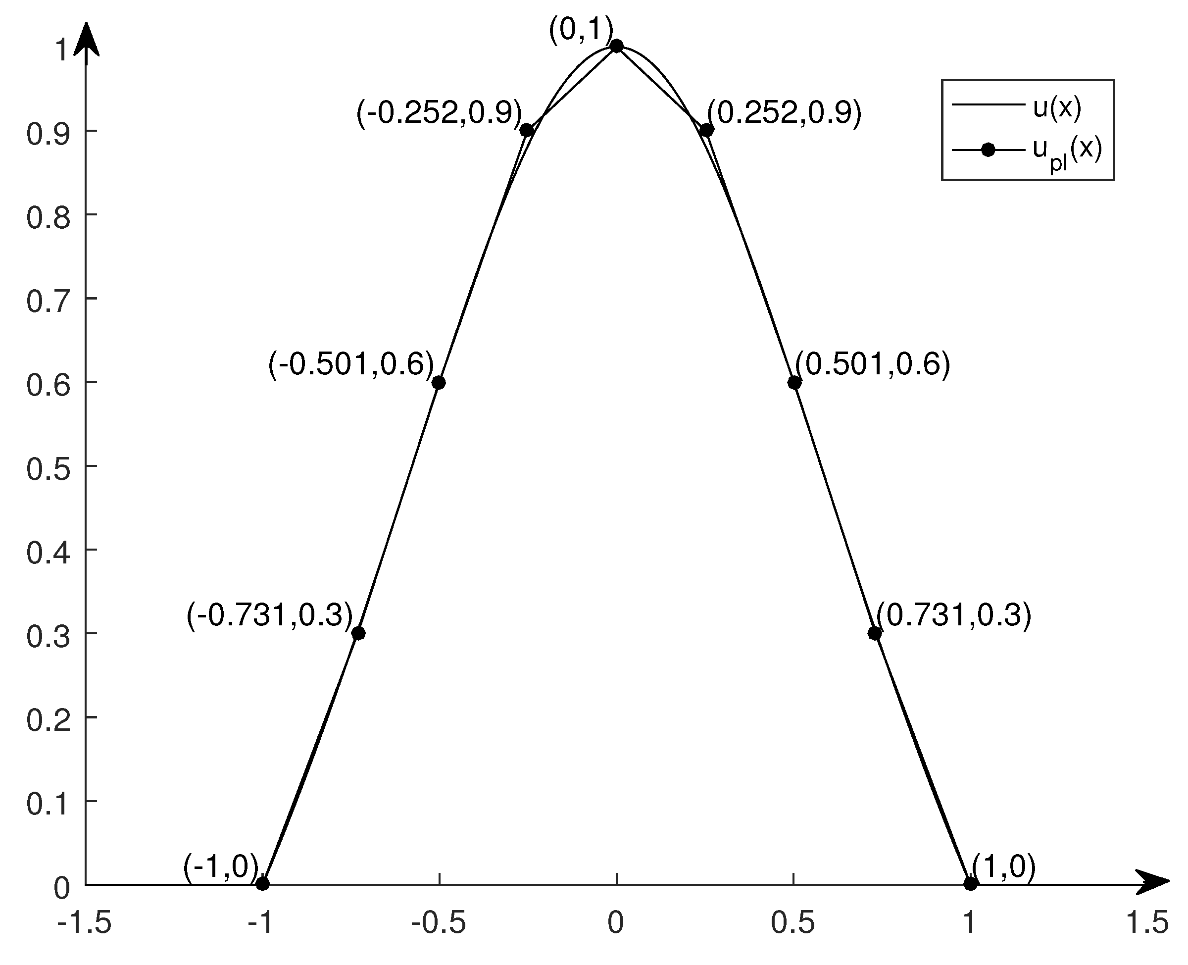
On the other hand, if we apply the methods (Formulas (11) and (12)) proposed in this paper, we can obtain that A   =   ( 1 , 0.731 , 0.501 , 0.252 , 0 ) and B   =   ( 1 , 0.731 , 0.501 , 0.252 , 0 ) . Therefore, by Theorem 1, we know that the piecewise linear fuzzy number (see Figure 3)
u p l   =   P L 1 0 0.731 0.3 0.501 0.6 0.252 0.9 0 1 ; 1 0 0.731 0.3 0.501 0.6 0.252 0.9 0 1
is the I-nearest ( 0 , 0.3 , 0.6 , 0.9 , 1 ) piecewise linear approximation of fuzzy number u, where A   =   ( 1 , 0.731 , 0.501 , 0.252 , 0 ) and B   =   ( 1 , 0.731 , 0.501 , 0.252 , 0 ) .
Remark 1.
Although the approximation effects of the two methods are not significantly different from Figure 2 and Figure 3, it should be admitted that, theoretically, the approximation method using weighted metric d * is better than that using unweighted metric d, and the approximation effect is better with the increase of the level threshold.
Example 2.
Let fuzzy number u be defined as
u ( x )   = ( x 1 ) 2 , x [ 1 , 2 ) 1 , x [ 2 , 3 ] 4 x , x ( 3 , 4 ] 0 , x [ 1 , 4 ]
By the definition of u ̲ ( r ) and u ¯ ( r ) , we have that u ̲ ( r )   =   1   +   r and u ¯ ( r )   =   4 r 2 and u ̲ ( 0 )   =   1 ,   u ̲ ( 1 ) = 2 ,   u ¯ ( 0 )   =   4 ,   u ¯ ( 1 )   =   3 .
If we take r   =   ( 0 , 0.2 , 0.5 , 0.8 , 1 ) and s   =   ( 0 , 0.3 , 0.6 , 0.9 , 1 ) , then by Formulas (11) and (12), we have that A   =   ( 1 , 1.476 , 1.710 , 1.897 , 2 ) and B   =   ( 4 , 3.927 , 3.656 , 3.201 , 3 ) . Therefore, by Theorem 1, we know that the piecewise linear fuzzy number (see Figure 4)
u p l   =   P L 1 0 1.476 0.2 1.710 0.5 1.897 0.8 2 1 , 4 0 3.927 0.3 3.656 0.6 3.201 0.9 3 1
is the I-nearest ( 0 , 0.2 , 0.5 , 0.8 , 1 ) ( 0 , 0.3 , 0.6 , 0.9 , 1 ) piecewise linear approximation of fuzzy number u.
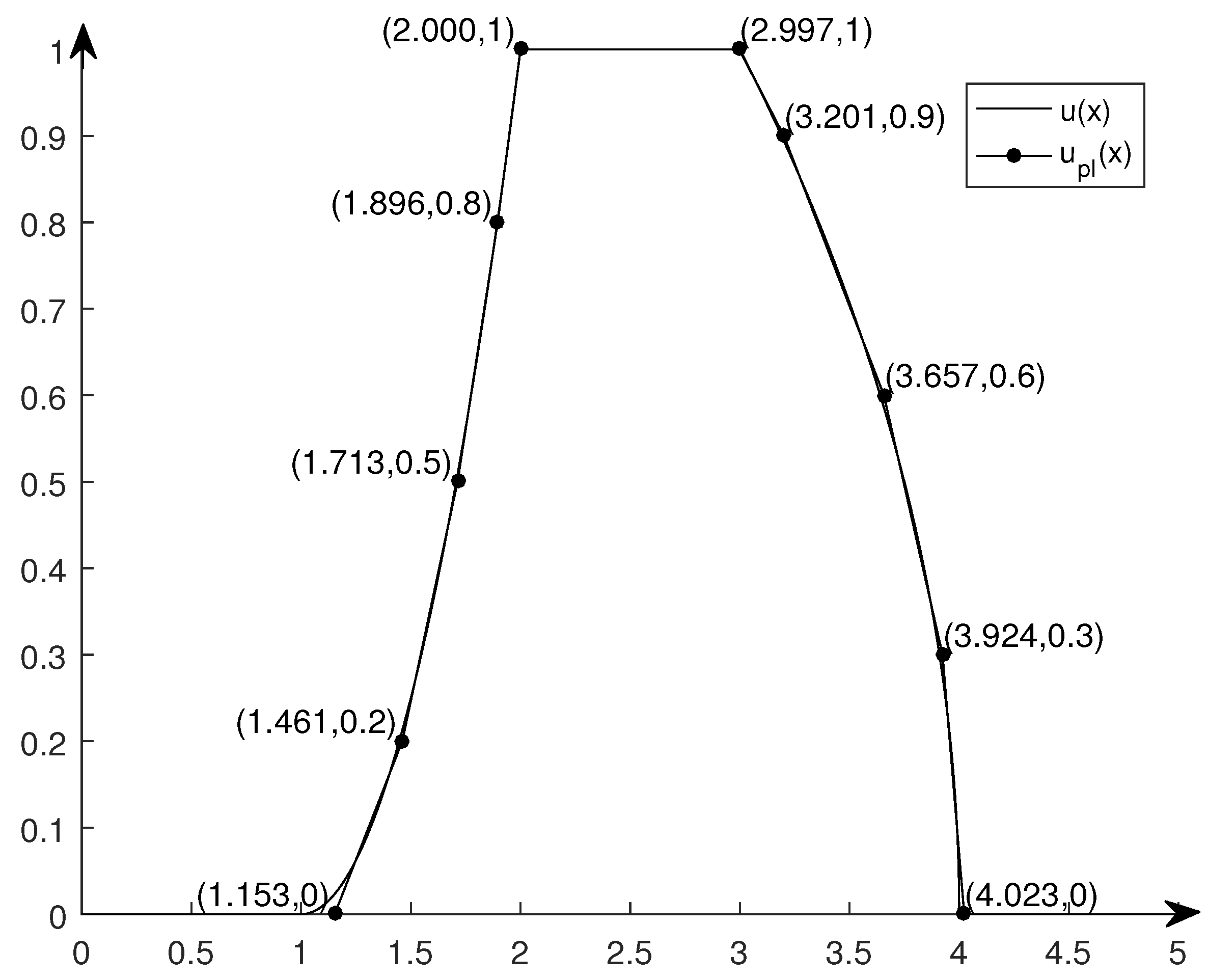
Likewise, by Formulas (19) and (20), we have that A   =   ( 1.153 , 1.461 , 1.713 , 1.896 , 2.000 ) and B   =   ( 4.023 , 3.924 , 3.657 , 3.201 , 2.997 ) . Therefore, by Theorem 2, we know that the piecewise linear fuzzy number (see Figure 5)
u p l   =   P L 1.153 0 1.460 0.2 1.713 0.5 1.896 0.8 2.000 1 , 4.023 0 3.924 0.3 3.657 0.6 3.201 0.9 2.997 1
is the II-nearest ( 0 , 0.2 , 0.5 , 0.8 , 1 ) ( 0 , 0.3 , 0.6 , 0.9 , 1 ) piecewise linear approximation of fuzzy number u.
Remark 2.
The difference between the I-nearest r-s piecewise linear approximation (Definition 1) and the II-nearest r-s piecewise linear approximation (Definition 2) is that I-nearest r-s piecewise linear approximation remains the same as the kernel of the original fuzzy number to be approximated, however, the II-nearest r-s piecewise linear approximation re-optimizes the kernel of the approximate solution. Through the comparison of Figure 4 and Figure 5 in Example 2, we know again that the method given in Theorem 2 is better than the method given in Theorem 1 for approximating a general fuzzy number by using piecewise linear fuzzy number.

5. Conclusions and Future Research Directions

In this paper, based on weighted metric d * , we give the definition (Definition 1) of I-nearest r-s (with respect to metric d * ) piecewise linear approximation and II-nearest (with respect to metric d * ) r-s piecewise linear approximation (Definition 2) for a general fuzzy number, and obtain the theorem (Proposition 1) of the relation between the two kinds of r-s piecewise linear approximations. Then, we obtain the method to get the I-nearest (with respect to metric d * ) r-s piecewise linear approximation (Theorem 1) and the II-nearest (with respect to metric d * ) r-s piecewise linear approximation (Theorem 2) for a general fuzzy number. Finally, we give a specific example to compare the new methods with approximation algorithms with respect to unweighted metric d (Example 1) and another example to show the effectiveness and usability of the methods proposed by us using weighted metric d * (Example 2).
In this paper, we establish a method to solve the best approximation when r and s are known. In the future, we can consider establishing a method to approximate a general fuzzy number with a simple fuzzy number when r and s are unknown. In addition, we can also discuss the approximation of high-dimensional fuzzy numbers.

Author Contributions

Conceptualization and methodology, H.L. and G.W.; formal analysis, investigation and writing—original draft preparation, H.L.; validation, supervision and writing—review and editing, G.W.; funding acquisition, G.W. All authors have read and agreed to the published version of the manuscript.

Funding

This work is supported partially by the Nature Science Foundations of China (Nos. 61771174 and U1934221).

Institutional Review Board Statement

Not applicable.

Informed Consent Statement

Not applicable.

Data Availability Statement

Not applicable.

Acknowledgments

The authors wish to thank the anonymous reviewers, whose insightful comments and helpful suggestions significantly contributed to improving this paper.

Conflicts of Interest

The authors declare no conflict of interest. The funders had no role in the design of the study; in the collection, analyses or interpretation of data; in the writing of the manuscript, or in the decision to publish the results.

References

  1. Treanţǎ, S. On a class of constrained interval-valued optimization problems governed by mechanical work cost functionals. J. Optim. Theory Appl. 2021, 188, 913–924. [Google Scholar] [CrossRef]
  2. Guo, Y.; Ye, G.; Liu, W.; Zhao, D.; Treanţǎ, S. Optimality conditions and duality for a class of generalized convex interval-valued optimization problems. Mathematics 2021, 9, 2979. [Google Scholar] [CrossRef]
  3. Fu, Y.; Xiao, H.; Lee, L.H.; Huang, M. Stochastic optimization using grey wolf optimization with optimal computing budget allocation. Appl. Soft. Comput. 2021, 103, 107154. [Google Scholar] [CrossRef]
  4. Zhang, S.; Chen, M.; Zhang, W.; Zhuang, X. Fuzzy optimization model for electric vehicle routing problem with time windows and recharging stations. Expert Syst. Appl. 2020, 145, 113123. [Google Scholar] [CrossRef]
  5. Zadeh, L.A. The concept of a linguistic variable and its application to approximate reasoning-I. Inf. Sci. 1975, 8, 199–249. [Google Scholar] [CrossRef]
  6. Zadeh, L.A. The concept of a linguistic variable and its application to approximate reasoning-II. Inf. Sci. 1975, 8, 301–357. [Google Scholar] [CrossRef]
  7. Zadeh, L.A. The concept of a linguistic variable and its application to approximate reasoning-III. Inf. Sci. 1975, 9, 43–80. [Google Scholar] [CrossRef]
  8. Ambrin, R.; Ibrar, M.; Delasen, M.; Rabbi, I.; Khan, A. Extended TOPSIS method for supplier selection under picture hesitant fuzzy environment using linguistic variables. J. Math. 2021, 2021, 6652586. [Google Scholar] [CrossRef]
  9. Mahmood, T.; Ali, Z. Entropy measure and TOPSIS method based on correlation coefficient using complex q-rung orthopair fuzzy information and its application to multi-attribute decision making. Soft Comput. 2021, 25, 1249–1275. [Google Scholar] [CrossRef]
  10. Ibrahim, H.Z.; Al-shami, T.M.; Elbarbary, O.G. (3,2)-Fuzzy sets and their applications to topology and optimal choices. Comput. Intell. Neurosci. 2021, 2021, 1272266. [Google Scholar] [CrossRef]
  11. Atef, M.; Ali, M.I.; Al-shami, T.M. Fuzzy soft covering-based multi-granulation fuzzy rough sets and their applications. Comput. Appl. Math. 2021, 40, 115. [Google Scholar] [CrossRef]
  12. Wang, C.Y.; Wan, L.; Zhang, B. Topological structures induced by L-fuzzifying approximation operators. Iran. J. Fuzzy Syst. 2021, 18, 141–154. [Google Scholar]
  13. Coroianu, L.; Stefanini, L. General approximation of fuzzy numbers by F-transform. Fuzzy Sets Syst. 2016, 288, 46–74. [Google Scholar] [CrossRef]
  14. Huang, H.; Wu, C.; Xie, J.; Zhang, D. Approximation of fuzzy numbers using the convolution method. Fuzzy Sets Syst. 2017, 310, 14–46. [Google Scholar] [CrossRef]
  15. Yeh, C.T.; Chu, H.M. Approximations by LR-type fuzzy numbers. Fuzzy Sets Syst. 2014, 257, 23–40. [Google Scholar] [CrossRef]
  16. Chanas, S. On the interval approximation of a fuzzy number. Fuzzy Sets Syst. 2001, 122, 353–356. [Google Scholar] [CrossRef]
  17. Grzegorzewski, P. On the interval approximation of fuzzy numbers. Commun. Comput. Inf. Sci. 2012, 299, 59–68. [Google Scholar]
  18. Grzegorzewski, P. Nearest interval approximation of a fuzzy number. Fuzzy Sets Syst. 2002, 130, 321–330. [Google Scholar] [CrossRef]
  19. Ban, A.I.; Coroianu, L. Symmetric triangular approximations of fuzzy numbers under a general condition and properties. Soft Comput. 2016, 20, 1249–1261. [Google Scholar] [CrossRef]
  20. Abbasbandy, S.; Hajjari, T. Weighted trapezoidal approximation-preserving cores of a fuzzy number. Comput. Math. Appl. 2010, 59, 3066–3077. [Google Scholar] [CrossRef] [Green Version]
  21. Khastan, A.; Moradi, Z. Width invariant approximation of fuzzy numbers. Iran. J. Fuzzy Syst. 2016, 13, 111–130. [Google Scholar]
  22. Coroianu, L.; Gagolewski, M.; Grzegorzewski, P. Nearest piecewise linear approximation of fuzzy numbers. Fuzzy Sets Syst. 2013, 233, 26–51. [Google Scholar] [CrossRef]
  23. Coroianu, L.; Gagolewski, M.; Grzegorzewski, P. Piecewise linear approximation of fuzzy numbers: Algorithms, arithmetic operations and stability of characteristics. Soft Comput. 2019, 23, 9491–9505. [Google Scholar] [CrossRef]
  24. Wang, G.; Shen, C.; Wang, Y. Approximation of fuzzy numbers by using multi-knots piecewise linear fuzzy numbers. J. Intell. Fuzzy Syst. 2020, 39, 3597–3615. [Google Scholar] [CrossRef]
  25. Grzegorzewski, P. Metrics and orders in space of fuzzy numbers. Fuzzy Sets Syst. 1998, 97, 83–94. [Google Scholar] [CrossRef]
  26. Zeng, W.; Li, H. Weighted triangular approximation of fuzzy numbers. Int. J. Approx. Reason. 2007, 46, 137–150. [Google Scholar] [CrossRef] [Green Version]
  27. Taussky, O. A recurring theorem on determinants. Am. Math. Mon. 1949, 56, 672–676. [Google Scholar] [CrossRef]
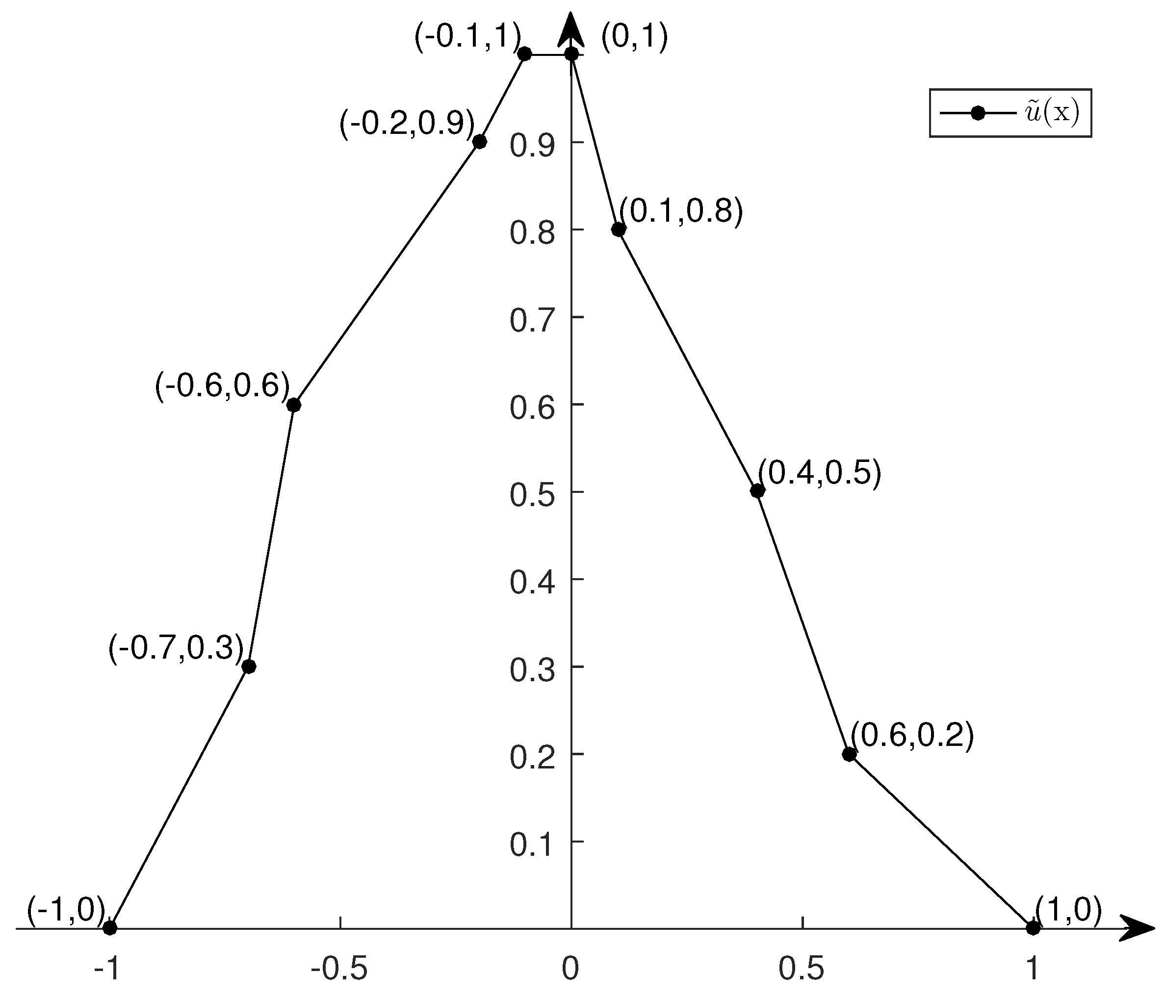
Figure 1. (0,0.3,0.6,0.9,1)–(0,0.2,0.5,0.8,1) piecewise linear fuzzy number u ˜ .
Mathematics 10 00145 g001
Figure 2. u and I-nearest ( 0 , 0.3 , 0.6 , 0.9 , 1 ) -KPLA u p l .
Mathematics 10 00145 g002
Figure 3. u and I-nearest ( 0 , 0.3 , 0.6 , 0.9 , 1 ) PLA u p l .
Mathematics 10 00145 g003
Figure 4. u and I-nearest (0,0.2,0.5,0.8,1)–(0,0.3,0.6,0.9,1) PLA u p l .
Mathematics 10 00145 g004
Figure 5. u and II-nearest (0,0.2,0.5,0.8,1)–(0.3,0.6,0.9,1) PLA u p l .
Mathematics 10 00145 g005
Publisher’s Note: MDPI stays neutral with regard to jurisdictional claims in published maps and institutional affiliations.