1. Introduction
Proteins from the same family have similar but also diverse functions [
1]. Hence, discovering conserved yet varied sequence patterns with various subgroup characteristics is important for understanding the protein functionality of a protein family. However, existing broad and imprecise grouping definition and processes neglect the diversity of certain protein families [
1]. One protein family may contain members that are strikingly variable in sequence length, three-dimensional structure, and hence biological function, where similar and diverse functional domains may reside in different sequence locations within the family. For example, class A scavenger receptors (SR-A) [
1], biologically important for binding on modified lipoproteins, are complex particles composed of multiple proteins that transport all fat molecules (lipids) around the body within the water outside cells to promote macrophage differentiation into foam cells, leading to chronic conditions such as atherosclerosis [
2]. SR-A is a diverse family of proteins classified based on their ability to bind modified lipoproteins [
3]. Although the five members (Marco, Sra, Scara3, Scara4, Scara5) [
1] of this family could bind modified lipoproteins, they are different in terms of their sequence patterns, locations, structures, and hence functions. For instance, within the same family, their protein length varies from 451 to 732 residues with the functional domains residing in different sequence locations. Thus SR-A is a protein family with conserved yet diverse function subgroups, ideal for exploration.
In order to reveal the functional subgroup characteristics of conserved sequence patterns corresponding to the diverse members of a protein family, we need mathematical transformations to disentangle the intriguing functionality related to conserved functional regions to reveal subgroups not explicitly manifested from the data. To this end, we have developed a novel method, known as Aligned Residue Association Discovery and Disentanglement (ARADD) [
4], based on our previous work Attribute Value Association Discovery and Disentanglement (AVADD) [
5], to discover and then disentangle the statistical representation of the Aligned Residue Associations (ARAs) derived from Aligned Pattern Clusters (APCs) for revealing their subgroups and subgroup characteristics.
In this study, we conducted experiments on SR-A, and found that the sequence patterns that are aligned and clustered into an APC via sequence similarity could be entangled in biological functions and domain location. Hence, we applied ARADD [
4] to disentangle the statistics so as to reveal the ARs and ARA Clusters (Patterns) corresponding to their functionality and residing location in the family. We further showed that even the ARAs captured in a Position Weight Matrix (PWM) [
6] discovered by the famous motif discovery MEME [
7] could be entangled in biological functions and domain location. We then demonstrated the effectiveness of ARADD [
4] in disentangling ARA patterns to reveal functional subgroups. The major contribution of our study is three-fold.
The focus of this paper, apart from introducing ARADD [
4] and emphasizing its novelty, is to produce a succinct analysis of subgroup characteristics obtained through pattern disentanglement, via the case study on SR-A. To our knowledge, no studies have reported similar experimental results.
The paper layout is as follows.
Section 2 does a literature survey.
Section 3 explains the methodology.
Section 4 describes the materials and
Section 5 illustrates the experimental results.
Section 6 outlines the biological significance.
Section 7 summarizes and concludes the research.
2. Related Work
Traditionally, computational sequence analysis methods have been developed to identify conserved sequence patterns from a protein family. Methods such as Multiple Sequence Alignment (MSA) [
8] are only suitable for globally homologous sequences with a high level of sequence similarity [
9], and motif discovery [
10]; another method, is based on probabilistic model (such as position weight matrix [
6]) which assumes independence between residue columns to represent the conserved sequence patterns. Such independence assumption is unrealistic in many cases, where correlation of residues along the sequence is commonly observed [
11,
12].
Pattern discovery is an essential element in predictive analytics [
13,
14] for knowledge discovery and analysis. Its essence is to discover patterns (motifs) occurring in the data to reveal association patterns for interpretation and classification [
15]. Hence, we develop an algorithm to obtain APCs [
16,
17] which capture functional residue association and site conservation. Since APCs contain aligned residues in strong statistical association sequence patterns, this representation is more knowledge-rich [
16,
17] when compared with MSA and probabilistic models. Hence, APCs reveal locally conserved yet diverse function patterns of protein families. APCs can reveal biological function in conserved regions of protein families.
Association rule mining [
18] is the most well-known methodology for mining item sets in relational dataset in the area of data mining. Algorithms such as Apriori [
19] and FP-growth [
20] can be applied for capturing associations from relational dataset. However, frequent patterns discovered by the above algorithms are extremely sensitive to threshold settings. Our new method, Aligned Residue Association Discovery and Disentanglement (ARADD), evolved from our AVADD [
5] method, and is proposed to solve this problem. ARADD is able to reveal residue association patterns in different orthogonal PCs and
Re-projected SRVs (RSRVs). ARADD is able to correlate different functionalities based only on the confidence intervals. As demonstrated in the results reported in this paper, ARADD achieves stable and succinct results in a simple fashion.
As observed in our recent paper [
5], a challenging problem encountered when discovering association patterns is that the association could be masked or obscured in the data due to the entanglement of unknown factors in their source environment. To resolve this problem for general relational datasets, we developed a novel method known as AVADD in our previous work [
5]. In this paper, we transformed the existing methodology to discover and disentangle ARAs from APCs. The reasons are as follows: (1) the aligned columns (sites) in an APC can be treated as attributes of relational dataset; (2) the residing residues on these sites can be treated as attribute values; (3) the residue associations in an APC can be treated as attribute value associations. The extended ARADD from AVADD [
5] could discover and disentangle ARAs from APCs as if AVADD [
5] could do that on
attribute value associations (AVAs) from a relational dataset. This is the most game-changing part of ARADD in comparison with existing methods. Due to such capability, subtle entangled subgroup characteristics masked or conspicuous in APCs can be revealed. To the best of our knowledge, only ARADD could disentangle such ARA patterns in APCs while no other reported methods could.
In summary, compared to the above-mentioned algorithms, ARADD solved the most difficult problems in discovering and analyzing subgroup characteristics of APCs containing entangled associations and the variation among them in their aligned sequence patterns. We should conclude that: (1) local associations may occur in different sequence locations or functional domains; (2) subgroups with similar patterns (motifs) could have small differences in functionality; (3) similar functionality may occur in different function groups and domains; and (4) multiple functionalities may occur within a functional group dominated by a key function. We refer to such entwined phenomena as the results of entangled ARA patterns.
3. Methods
The method used in this paper is evolved from AVADD [
5], which was developed by our team. It was used for discovering and disentangling AVAs from mixed-mode relational datasets (RDS) [
5] very successfully. In this study, we extended AVADD to discover and disentangle the statistical representation SRV of the ARAs obtained from APCs to reveal their subgroups and subgroup characteristics as well as to locate their functional domains.
By Aligned Pattern Cluster (APC) [
16,
17], we mean an array of sequence segments containing a cluster of aligned statistically significant sequence patterns grouped together according to their similarity though alignment [
16,
17].
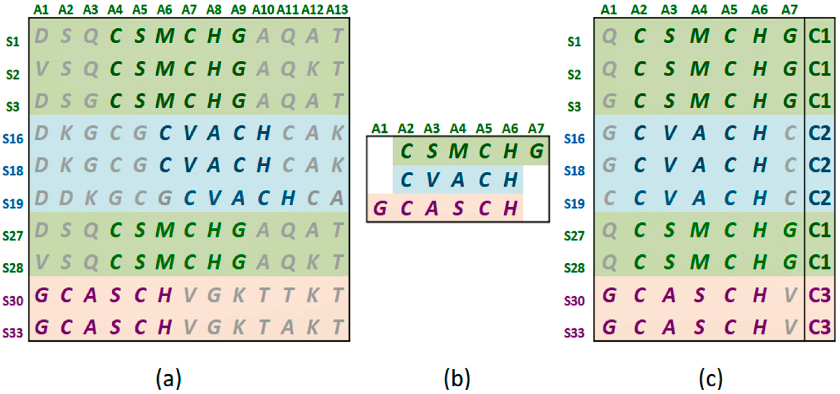
Figure 1a shows the statistically significant sequence patterns discovered from the sequence data.
Figure 1b represents the pattern space of the APC when the discovered patterns are aligned.
Figure 1c is referred to as the data space of the APC showing all the sequence data segments containing the patterns in the APC with their pattern sequence ID and head position registered. Through the data space of APCs, any ARs or ARAs of an APC identified in any PCs and RSRVs, respectively, can be located.
Figure 2 shows the three major steps of ARADD. (1) ARADD converts an APC into an ARA Frequency Matrix (ARAFM) (Definition 1). It then converts the ARAFM into an Adjusted Statistical Residual Space (SRV) so that each frequency entry in ARAFM is transformed into a Statistical Residual (SR) that accounts for the deviation of the frequency of occurrences of the ARA from the expected frequenting if the associations were random. In the SRV, each row represents a vector of an AR (referred to as an AR-vector or a-vector) whose coordinates represent the SRs of that AR associated with other ARs corresponding to the column AR-vectors; (2) Next, ARADD conducts the Principal Component Decomposition on the SRV to obtain the top Principal Components (PCs) ranked according to their variance, and then projects all the AR-vectors in the SRV onto the PC axis. The new SRV containing the vector projections on the PC is referred to as the Re-projected SRV. The new set of coordinates of these projections reflects the SRs of that AR associating with other ARs corresponding to the column vectors; (3) Finally, for each PC, ARADD identifies the distinct ARs and/or AR clusters with variance ≥1.0 from the center and then obtains the SR value of the ARA between the ARs within each AR clusters in the RSRV to reveal the association patterns.
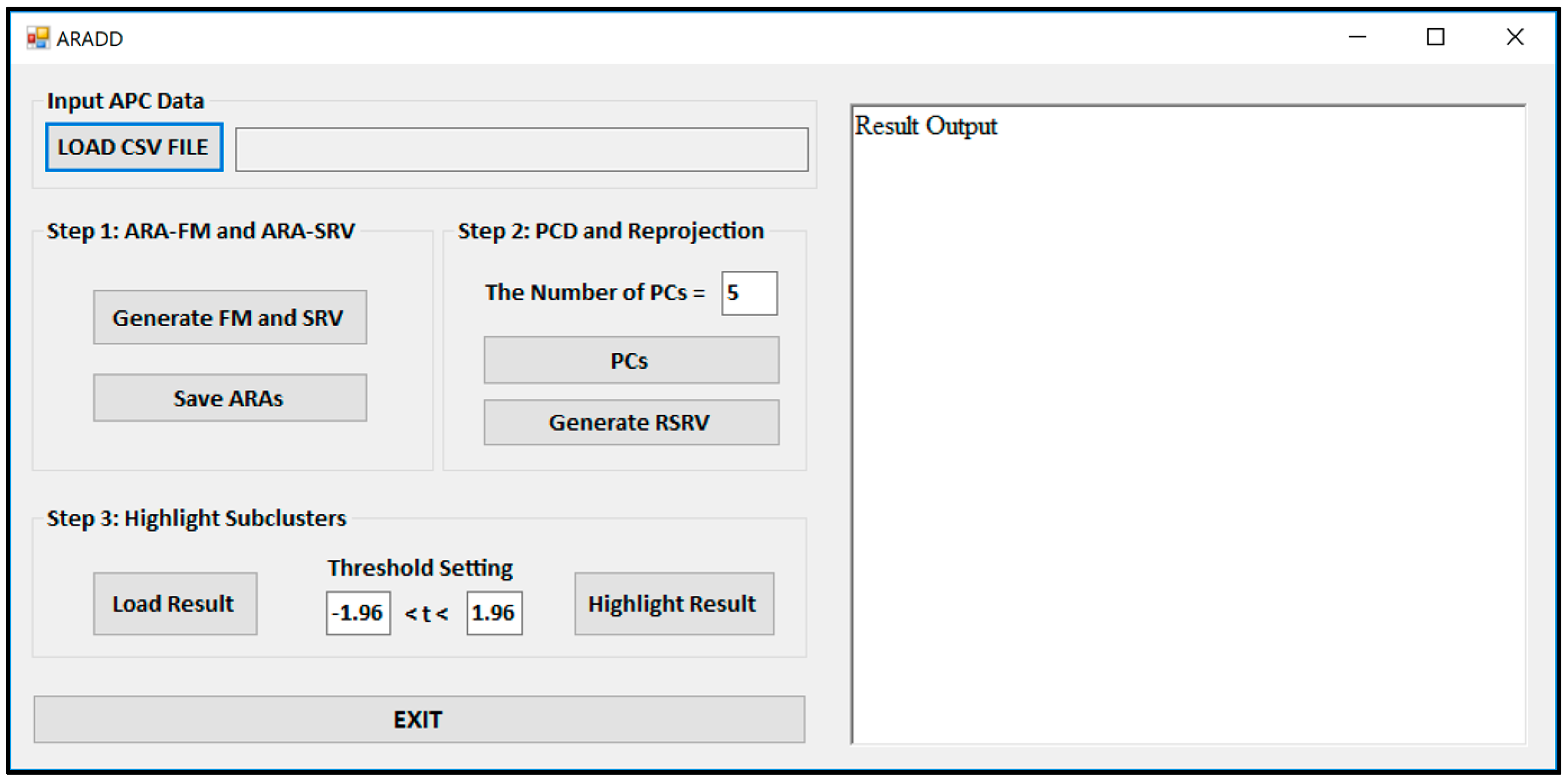
Figure 3 shows the Graphical User Interface (GUI) of the ARADD software. After loading the CSV file of an APC; pushing the button labeled “Generate FM and SRV” will create both the ARAFM and SRV for the APC. The process in Step 2 will generate the set of top PCs and their corresponding RSRVs according to the number of PCs or percentage of the variance assigned in the box. The process in Step 3 will highlight the sub-cluster results according to the assigned confidence interval in the box.
We can represent an APC dataset by M amino acids (residues) on N amino acid sites, denoted as A = {}. Each amino acid site can assume a categorical value as a residue type. Thus contains values, denoted as . Hence, I = represents the total number of residue types (values) of all sites in an APC.
ARA represents the residue associations between residues on different aligned columns of the APC (i.e., the residue pairs). The ARA, represent the residue association between two aligned residues with the aligned site positions n and n’ and the residue types i, j respectively.
Definition 1. ARA Frequency Matrix. An ARAFM is a matrix of frequency counts of ARA between two aligned amino acids (residues) on two aligned sites, say , within the same protein sequence. We denote the frequency by , where represents the residue of ith type on the nth aligned site in the APC, and represents the residue of the jth type on the n′th aligned site (n ). Hence, ARAFM is an I I matrix.
Now we shall describe the operations associated with each step in the ARADD GUI.
Step 1: Construct Adjusted Statistical Residual Vectors Space (SRV):
The button “Generate FM and SRV” in
Figure 3 is used to construct the ARAFM first and then to convert the ARAFM into SRV (Definition 2).
Definition 2. ARA Adjusted Statistical Residual Vector Space. An SRV is a vector space such that the jth jjas coordinate of its ith iithat row vector (a-vector or more precisely vector), corresponding to the ith type residue on the nth site in the APC. We denote the n’ coordinate of the vector by which is the SR obtained from Hence, an SRV can be expressed as a set of row vectors: SRV = <
>, where I = is the total number of ARAs, and is the total number of unique SRs for the first aligned column (), and is the number of unique amino acid for the nth aligned column (). An a-vector is hence denoted as = ),… ),… )}, where ) represents the statistical residual for ARA (), and ) = 0.
By replacing each ARA frequency with its Adjusted Standard Statistical Residual (SR), we can construct the SRV. We treat SRV as a vector space such that each row is taken as a row vector (AR-vector or a-vector) with its coordinates representing the SR of its ARAs associating with other ARs denoted by the column a-vectors.
To obtain statistically significant information from an APC, we transform an ARAFM into a SRV by converting each ARA frequency
into an SR, denoted as
).
where
represents the total number of occurrences when
and
;
=
, where
represents the total number of counts when
represents the total number of counts when
and
M is the total number of records.
To reveal the statistical significance of an ARA, here,
measures the deviation of the observed frequency,
, of the ARA from its default model
assuming that the occurrence is a random association. Unlike the standardized residual, the Adjusted Statistical Residual considers the overall size of the sample and gives a more accurate indication of how far the observed count is from the expected count. So, in this paper we abbreviate Adjusted Statistical Residue as “
SR”, to be consistent with our previous paper [
5]. We denote
SR as
), which is the significance of ARAs. The value of
is calculated using Equation (2).
Here, is the maximum likelihood estimate of the variance of , and is defined as: = () × (). We should note that the respective statistical thresholds for significant and insignificant ARAs remain unchanged.
Although the SRs can reveal the significance of an ARA, subtle associations could still be entangled and masked. Hence, by treating the ARA SR matrix as a SR vector space (SRV), we have developed a novel method to disentangle the SRV through Principal Component Decomposition (PCD) onto a set of PCs and reproject the projections of the AR-vectors on each PC back to a new SRV referred to as its corresponding RSRV.
Step 2: Conduct PCD on SRV and Obtain for Each PC Its Corresponding RSRV.
The button “PC” in
Figure 3 is used to initiate the application of the PCD (Definition 3) on the SRV and obtain a number of top PCs according to the number (or the threshold of the total variance) set in the window. In the meantime, in order to disentangle the discovered AVAs from SRV, the a-vector projections on each PC is re-projected onto a new SRV, referred to as the Re-projected SRV (Definition 4). The new transformed a-vector positions in the RSRV correspond to a new set of ARA SRs for each AR with other ARs in the RSRV. These new positions of a-vectors reflect the ARAs captured in the corresponding PC.
Definition 3. Principal Components. In PCD, PCs are a set of k PCs, denoted as PC = {, where is a set of projections of the a-vectors from SRV, denoted as = {}, where N is the total number of all aligned columns in APC and is the total number of distinct amino acids on the column .
Definition 4. Re-projected SRV (RSRV). RSRV is the SRV containing the a-vector projections on a PC. The coordinates of an a-vector projection on the PC in the RSRV represent the ARA SRs of the AR of that a-vector associating with other ARs corresponding to the column vectors as captured by the PC (Equation (3)). After PCD, we first identify the distinct projection(s) of the a-vectors and their furthest clusters from the mean (center) of the PC-Axis. The a-vector projections in PCs with large eigenvalue should have strong association or strong presence captured by the orthogonal PCs.
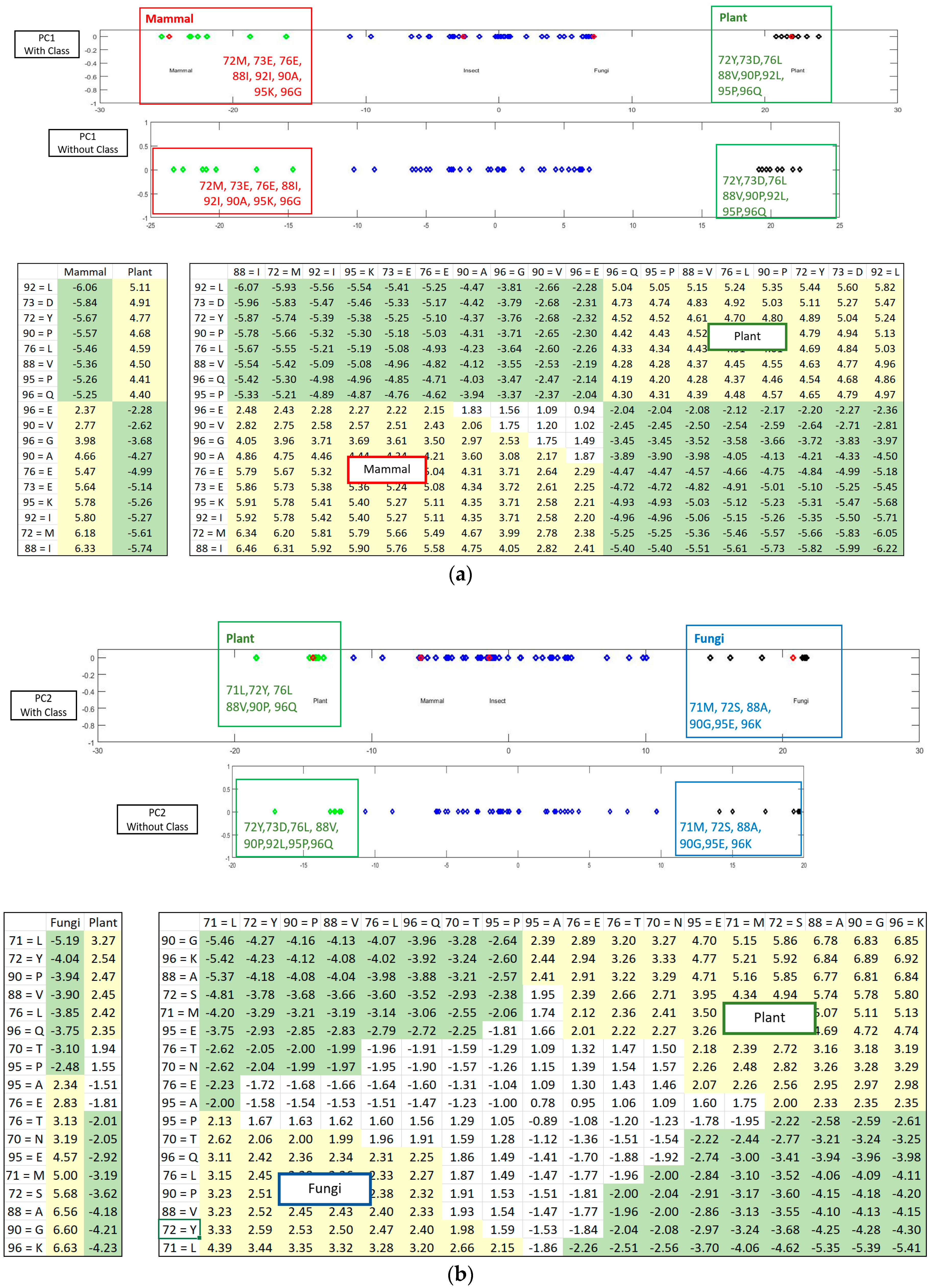
If the class labels are included in the APCs, its position in the PCs appears just as a virtual AR (essentially the centroid of the ARs within an AR cluster pertaining to that class). In the illustrative example in
Figure 4, the colored dots enclosed in the square boxes are centroids of the AR clusters associated to specific classes like mammal, plant, etc.
Hence, the new positions of the projections of the a-vectors on the PC, when transformed to the SRV, represent the a-vectors with a new set of coordinates in the RSRV. We mark the correspondence by attaching to them the same subscript, i.e., k in PCk and RSRVk.
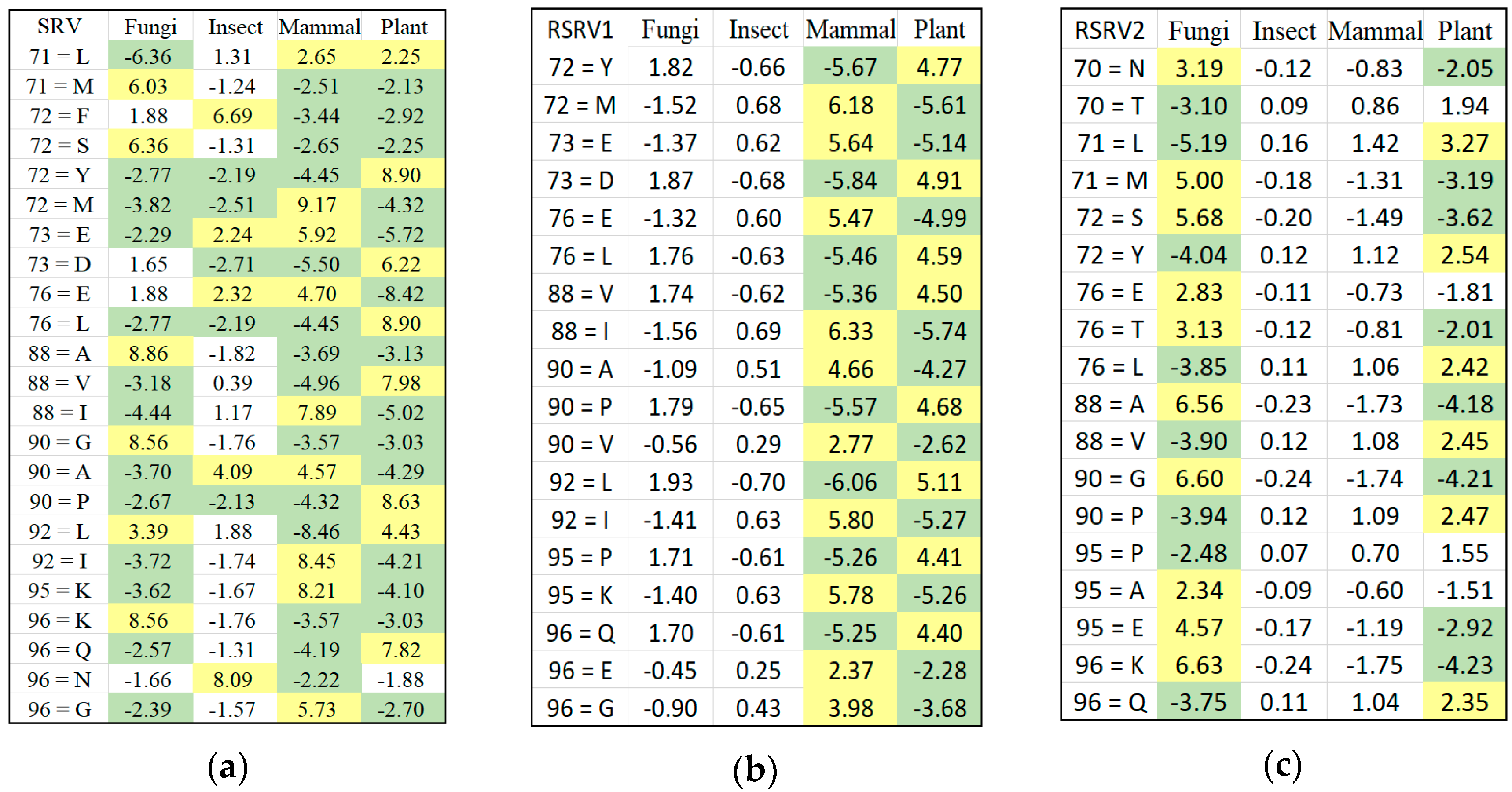
Figure 5 shows how the SRV with AVAs, related to the taxonomical subgroups and obtained from APC-6382 (described later in the Results Section), is disentangled into different RSRVs (such as, RSRV1 and RSRV2) and thus revealing ARA subgroups corresponding to different functionality pertaining to the taxonomical classes in the region. Note that the ARAs entangled in SRV (
Figure 5a) are disentangled into succinct sub-groups corresponding to difference taxonomical classes in RSRV1 and RSRV2 (
Figure 5b,c, respectively).
To summarize this step, PCD uses an orthogonal transformation to transform a set of possible correlated variables into a set of linear uncorrelated variables known as PCs. The first PC, , has the largest possible variance, which accounts for ARs with the highest ARAs with other ARs. PCs with less variance follow.
Step 3: Identify Distinct ARs and AR-Clusters Through Their Statistical Significant ARA SRs Between ARs.
The button “Highlight Result” in
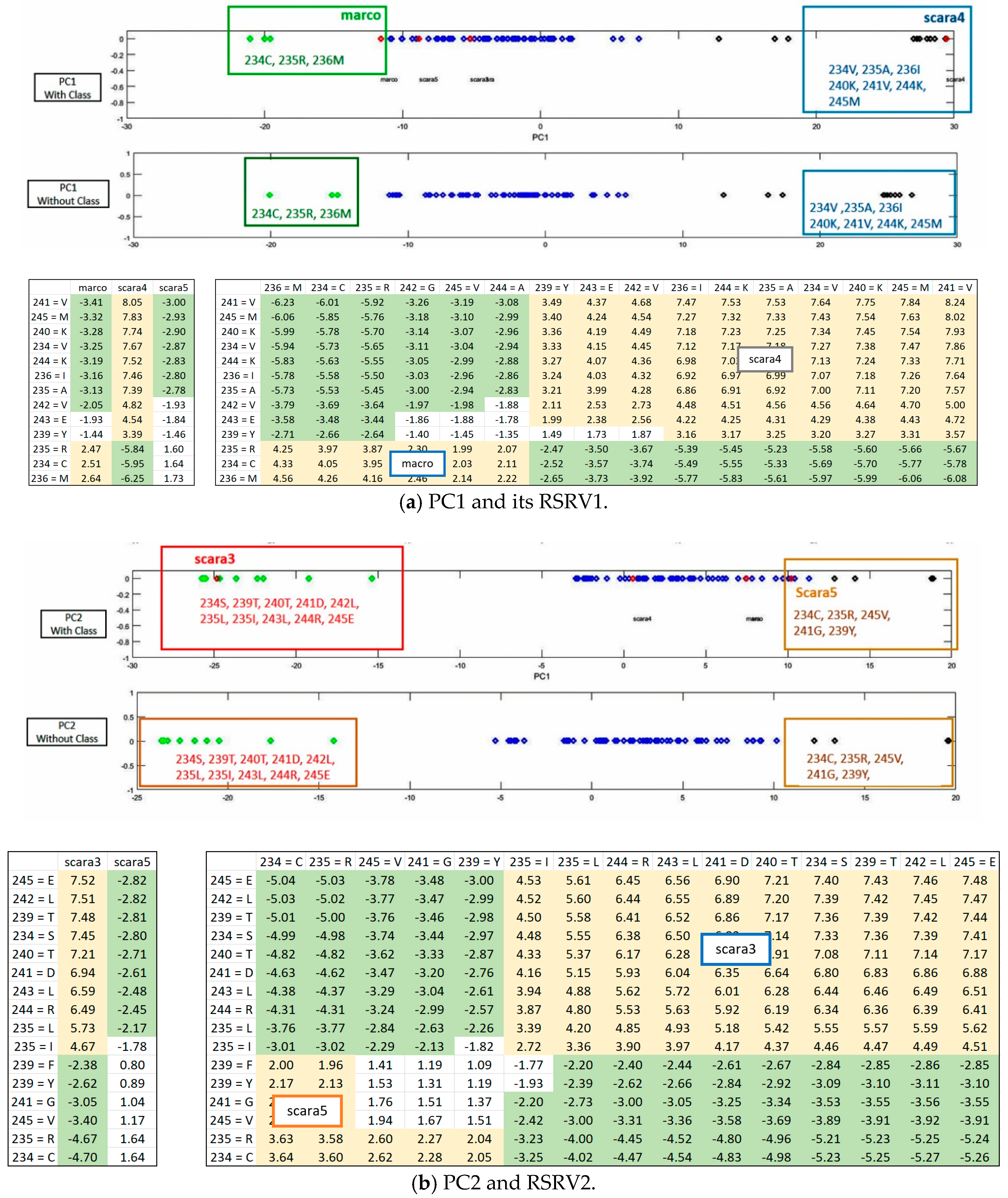
Figure 3 is implemented for highlighting the results from the sub-clusters. When a cluster of ARs forms an association pattern, they should share strong ARAs. By setting the threshold to 1.96, the strong ARAs can be grouped together to represent an AR sub-cluster in the RSRVs. A careful comparison of the PCs (
Figure 4) and their corresponding RSRVs (
Figure 5) shows that the distinct AR clusters captured in PCs are reflected by the statistical significant ARAs in their corresponding rows (a-vectors) in the RSRVs (yellow cells). More succinct representations are found in
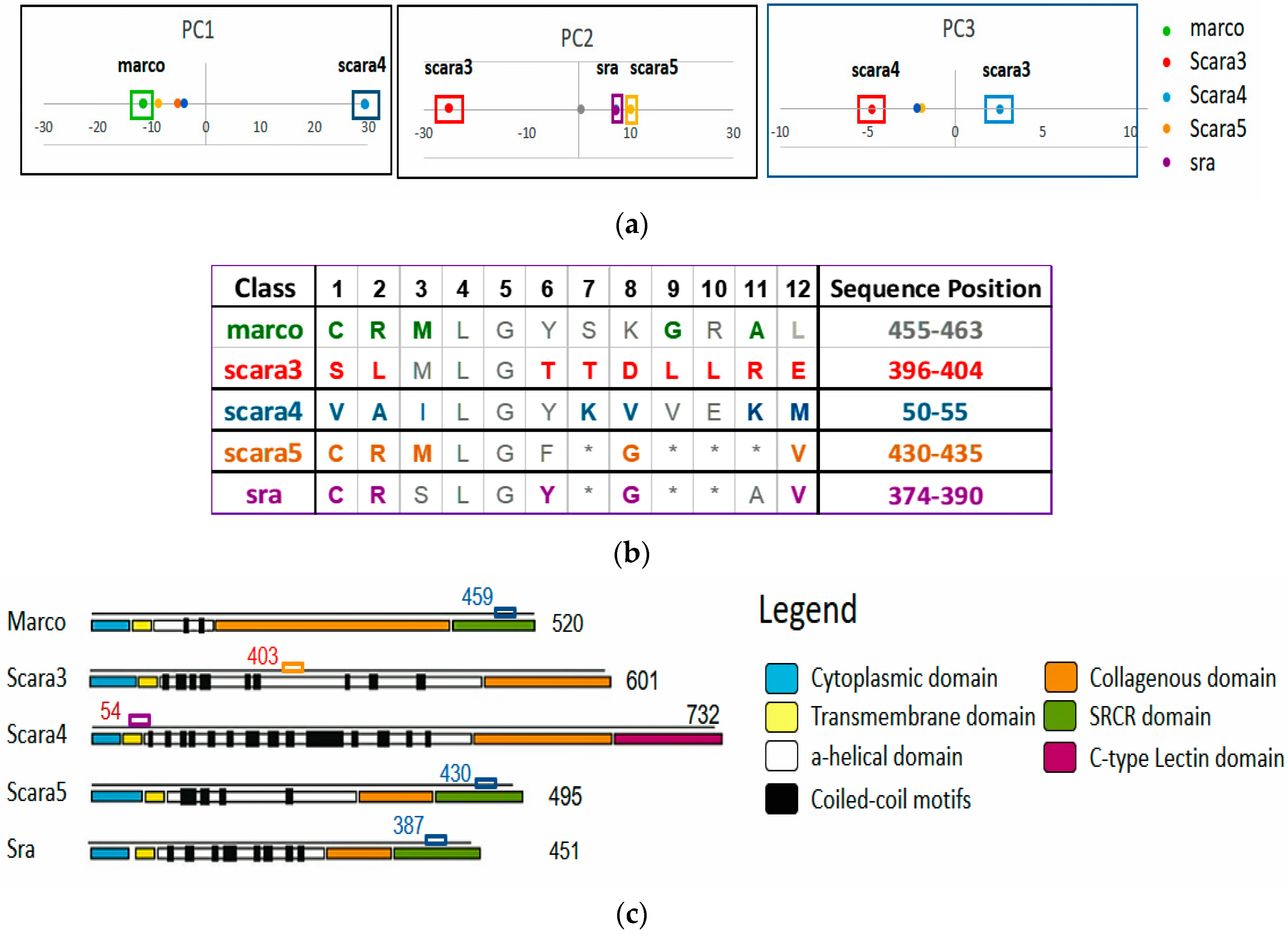
Figure 6 and
Figure 7.
Output: RSRVs and ARA Sub-Clusters
Disentangled ARAs by distributing and grouping them in different RSRVs. After PCD, it may not be obvious why an a-vector is significant. However, when the a-vectors are examined in the RSRVs, it can be observed that their high SR coordinate(s) contributed to their high variance on their corresponding PCs. In general, PCD is sensitive to the relative scaling of the original aligned columns. By unifying the scaling of ARA measures through SR, our results showed that SRV is rather stable and can reveal statistically significant associations between ARs with statistical strength reasonably well. However, when ARAs become entangled, the SRV disentanglement is crucial for yielding highly distinct, stable, and specific results as manifested in the RSRVs obtained from both datasets (
Figure 4,
Figure 5,
Figure 6,
Figure 7 and
Figure 8).
ARs Sub-clusters. Although the disentangled PCs can already reveal significant ARs/AR-Clusters on a one-dimensional space (
Figure 4,
Figure 6 and
Figure 8), the statistical strength (SR) of the ARAs can further reveal the significance of the ARAs and the AR-Clusters by identifying their RSRVs through the SRs from the row and column a-vectors (RSRV1 and RSRV2 on bottom half of
Figure 6a,b and
Figure 7a,b. By disentanglement, we can obtain different ARs sub-clusters in different orthogonal PC spaces as shown in both figures. These AR subgroups may have functional meaning. They may help to build classification or subgroup partitioning models with less features but can achieve comparably superior performance to the classification models based on statistical significant ARAs derived from SRV. Furthermore, it is much easier to select discriminative features from RSRVs after disentanglement than from SRV and from the distinct ARs and AR clusters in the PCs.
