1. Introduction
Online education has been around for some decades, even though the breaking point for its massive adoption was the COVID-19 pandemic back in 2020 (
Shrestha et al., 2025). The public health emergency brought by the pandemic made it impossible to continue with face-to-face lectures at any education level and led to an abrupt paradigm shift in favor of remote online learning in order for teachers to keep delivering classes to learners (
Baxter & Hainey, 2023).
Online education is actually an evolution of distance education through the use of information and communication technologies (ICTs). In fact, correspondence education could be seen as a forerunner of online education, which has been around for centuries, where instructors and students exchanged materials and assignments by post mail (
Moore, 2023). Likewise, the continuous advances in technology in the twentieth century made remote education evolve, thus including communications between instructor and students via telephone, radio, television, and personal computers (
Betts et al., 2021). However, in the twenty-first century, personal computers have been sharing their prominent position in distance learning with mobile computing devices, such as laptops, smartphones and tablets (
Eom, 2021).
Online education could be described as the use of digital devices in order to provide online lessons (
Singh & Thurman, 2019). However, the context of the different areas did make a difference regarding the access to technologies or devices, the knowledge of the platforms being used, and the methodologies adopted by each teacher (
Tadeu et al., 2023). On the other hand, the lack of digital literacy or belonging to a particular socioeconomic group were factors that may lead to lower results in online education (
Klosky et al., 2022). Likewise, the accessibility to educational and technological resources greatly differed depending on the country, which posed some questions about the responses to remote education depending on the location (
Bond et al., 2021).
Looking back on remote education in the pandemic times, it is clear that there was a lack of planning to move from a traditional face-to-face education to online education (
Stewart & Lowenthal, 2023). In that context, online learning activities and assessments were often improvised, although the results obtained were quite positive in the circumstances due to the pandemic (
Broadbent et al., 2023). Furthermore, the flexibility offered by online education has been corroborated in subsequent studies in the literature, such that the option of offering purely online education has been contemplated in some cases, whereas combining online and in-place learning experiences has been considered in diverse educative levels (
Ali et al., 2020;
Krzyzak & Walas-Trebacz, 2024;
Chaves et al., 2025;
Fialho-Capellini et al., 2025).
In this paper, a scheme for combining online learning with in-site learning has been put in place in a college course in the current academic year. Such a scheme results in a specific set of combinations regarding the location where the learning is acquired, the moment when the learning is acquired, and the language in which the learning is acquired. Hence, the research question in this paper is whether the change in settings related to space, time, and language for the learning process would affect its outcome, compared to the results achieved in the previous academic year where a traditional education scheme was in place. Additionally, the research goal in this paper is to measure the differences between the outcomes achieved in both academic years.
The motivation for the implementation of this kind of methodology where the dimensions related to space, time, and language were constantly changed in each session was twofold. The first one was to assess how the students would react to such a disruptive scheme put in place in this experimental course, where those dimensions were constantly changed. The second one was to evaluate how the academic performance of students would differ in this context compared to the academic performance achieved by previous students where the same course was taught in a traditional education way.
On the one hand, students’ reaction was assessed both quantitatively and qualitatively, where the former was implicitly attained out of the increase or decrease in academic performance comparing this current course and the previous one, whereas the latter was achieved by receiving comments from students about how the combinations of space, time, and language contributed to their learning experience. As a matter of fact, most students initially found it hard to get into a routine, even though they eventually got used to it. On the other hand, the latter was checked out by confronting the scores obtained in both courses regarding the academic performance.
As a consequence, the reason for this type of changes in the dimensions within a course was also twofold. The first one was to test how students would adapt to unforeseen events, whilst also trying to get them prepared in case any unplanned situation would arise during a course. In fact, one of the lessons learned from pandemic times was the need to prepare contingency plans in order to respond as effectively as possible in case of an emergency. Hence, we considered to set up this scheme as a test to get ready for unexpected events. The second one was to measure whether those changes in the dimensions of a course could have an impact in academic performance compared to previous results obtained where dimensions were kept steady throughout a course.
The course in which this scheme of changing dimensions was implemented corresponds to a college course dedicated to Introduction to Computer Science. This is considered a STEM course, as it fits in the engineering field, specifically in the basics of computer engineering. It should be noted that such students are supposed to be used to working with computers and the internet, thus they are meant to have the necessary technical skills to properly adapt to the changes proposed in this experimental course, which somewhat simplifies the adaptation period to the layout of this course.
Additionally, this experimental setup favors the deployment of active learning activities, where students may have a more prominent role in their education process. Actually, the deployment of not only individual activities but also group activities in either on-site, online or mixed environments could facilitate an active role for students, while teachers could play the role of a facilitator. This way, not only technical skills are acquired by learners, but also soft skills, such as collaboration, communication, or leadership. Hence, some active learning setups were included in the different sessions in order to keep students actively engaged during the different sessions. In this sense, group discussions were encouraged regardless the settings established for each session in order to keep students engaged.
The dependent variable considered in this experimental course will be the student outcomes. The reason for this is because they have to take a series of exams in order to pass the course, so it is straightforward to obtain all those grades. At that point, the grades will be statistically processed in order to attain the most common descriptive statistics for the experimental course. After that, these descriptive statistics will be compared to the corresponding figures achieved in the previous year with a traditional course in order to check whether the new setup achieves better learning outcomes or otherwise.
Furthermore, inferential statistics will be applied to the descriptive statistics achieved in both years in order to check if the improvement or the setback experienced was statistically significant, along with finding the corresponding effect size and sample size. Apart from these quantitative data about the experimental course, some qualitative data will be obtained by asking the students about the contribution of the combinations of space, time, and language to their learning experience.
3. Methods
First of all, the dimensions considered in this paper are described, followed by the context of the current study. After that, the setup of the course structure is exhibited, and finally, the implementation tools are outlined.
3.1. Dimensions
Among the multiple characteristics being part of the teaching/learning process, in this study we are focusing on just three dimensions. Those are the location (space) where the students access the contents, the moment (time) when the students access the contents, and the coding system (language) in which the contents are imparted (
Zadeh et al., 2022). In other words, those dimensions respond to the following questions about learning the contents: where, when, and how.
If those three dimensions are considered the axes in a Cartesian coordinate system, then a three-dimensional Euclidean space is obtained. However, if only positive values are allowed for each dimension, then only the positive octant of the whole 3D-space is considered. It should be noted that the concept of octant is analogous to a quadrant in a two-dimensional Euclidean space, or a ray in a one-dimensional Euclidean space, which accounts for a line segment extending to the infinite at one end.
Hence, considering a given learning session with a certain setup related to space, time, and language, each of those dimensions could be coded with a particular value according to its corresponding setting. Putting those three values together leads us to associate them with a triplet, which depends on the feature selected for each dimension (
Sánchez-Puig et al., 2024). For all three dimensions, the value 0 is given to the traditional scenario, the value 1 is given to the innovative scenario, and the value 2 is given to the hybrid scenario, where both options are available for students, namely, values 0 and 1 at the same time.
This way, regarding the space, the value 0 is assigned to in-person, whereas the value 1 is assigned to online, and the value 2 is assigned to a combination of both, which is often referred to as blended (
Sun & Zhang, 2023). Regarding the time, the value 0 is associated to synchronous, whereas the value 1 is associated to asynchronous, and the value 2 is associated to a combination of both, which is often referred to as bichronous (
Martin et al., 2023).
Regarding the language, the value 0 is tied to lessons taught in the primary language, which will be typically the common official local language used in the education system, whereas the value 1 is tied to lessons taught in the secondary language, which will typically be the English language because it is currently the ‘lingua franca’. However, in some regions with two local languages, it could also refer to the other official language used in the education system. In any case, the value 2 is tied to lessons taught in a bilingual scenario. This could be implemented in different ways, such as a simultaneous translation of the lecture to the other language, or otherwise, as the use indistinctly of both languages in the lecture (
Mortimore, 2024).
Therefore, as there are 3 different dimensions, where each of them may have 3 values available, then an overall amount of
scenarios could be set up, where all combinations are possible, although some of them are more common than others (
Roig et al., 2024a).
Figure 1 depicts the positive octant of a 3D Euclidean space, where values 0, 1, 2 are assigned to each axis, and the order of a given triplet is (space, time, language).
For instance, the traditional teaching/learning process is widely identified with a masterclass delivered by a teacher within a classroom. In this context, the teacher carries the active role, while the pupils bear a passive role, meaning that they just listen to the lecture, even though they may at some point ask some questions about it.
Looking deeper into the scenario of traditional lecture, the spatial dimension is in-person, as students are at the same location as the teacher, whereas the temporal dimension is synchronous, as students attend the lesson at the time the teacher delivers it, and the language dimension is local, as the lecture is delivered in the local language. Hence, the triplet related to traditional lecturing is (0,0,0). However, if the traditional lecture is delivered in foreign language, then the associated triplet becomes (0,0,1), whereas if both languages are used, then the attached triplet is (0,0,2). Analogously, any other combination of the values available within the triplet could also be worked out.
Furthermore, the dimensions considered in this study may well be considered variables in order to carry out the operationalization of variables, which means to define them in a way that allows their accurate measurement (
Andrade, 2021). According to the description of the dimensions made above, all of them were expressed in terms of discrete values, namely 0, 1, and 2, even though the specific meanings differed for each particular dimension. Hence, in this case, those discrete values imply categorical variables, as opposed to continuous ones, as no intermediate values are allowed. Alternatively, categorical values are also considered qualitative ones, whereas continuous values are also taken as quantitative ones.
Moreover, each dimension takes values according to its own specific categories. In this sense, the spatial dimension can be taken as on-site, on-line, and blended, while the temporal dimension can be taken as synchronous, asynchronous, and bichronous, whilst the linguistic dimension can be taken as local language, foreign language, and bilingual.
Table 1 displays the operationalization of variables (
Arias-Gonzáles, 2021), considering the dimensions related to space, time, and language as variables.
3.2. Context of This Study
This college course dedicated to Introduction of Computer Science was attended by 30 students in the current academic year, namely 2024–2025, and also in the last academic year, namely 2023–2024. The attendants in both editions were ranged between 18 and 25. Regarding the gender of the attendants, in the edition held in the previous year there were 9 women and 21 men, whereas in the edition held in the present year there were 10 women and 20 men, thus there was just a slight difference.
The college was based in Spain, so the official language of tuition is Spanish. Hence, Spanish language is considered the local language. On the other hand, English language is considered the foreign language because it is the common language for knowledge exchange at an international level. Therefore, bilingual is going to be considered the combined used of Spanish and English in a session. Consequently, if a session is imparted in Spanish, the corresponding value in the third position within a triplet will be 0, whereas it will be 1 if a session is taught in English, and it will be 2 if a session is bilingual, where Spanish and English are both used.
On the other hand, it should be said that the usual language in the sessions of our college is the local language, which is Spanish. Hence, this is the case in most situations. However, there are some specific courses run in English due to different circumstances, such as the presence of a visiting foreign teacher who is not fluent in Spanish, or a given course specifically established in English. Nonetheless, this experimental course was set up with the aim of providing different options for the linguistic dimension in order for students to adapt to different environments during their education, which may well happen once they join the labor market after finishing their studies.
3.3. Setting Up the Course Structure
The deployment of those combinations of active learning setups have been undertaken in a course on Introduction to Computer Science in the current academic year, namely 2024–2025. This course was also taught in the last academic year, namely 2023–2024, with a traditional teaching approach, thus based on masterclasses imparted by the teacher. The organization of the course in the present academic year has involved the application of a different combination of active learning for each of the 12 sessions within the course.
Table 2 exhibit the combination assigned to each of the sessions.
The 12 sessions have been grouped into sets of 3 sessions, where the values for two dimensions are fixed for all those sessions, whereas the value of the other dimension differs in each particular case, thus taking all values allowed for that unfixed dimension.
Regarding the first set of three sessions, which involves those identified 1, 2, and 3, they share the same value for space, namely blended, such that attendants are both in-person and online, and they also have the same value for time, namely synchronous, such that attendants can access the sessions only live. On the other hand, the value for language varies in each session, such that the first one is taught in local language, the second one is taught in foreign language, and the third one is taught in both languages, even though students might obtain the help of instant translators through specific applications.
With respect to the second set of three sessions, which involves those identified 4, 5, and 6, they share the same value for space, namely blended, such that attendants are both in-person and online, and they also have the same value for time, namely asynchronous, such that attendants can only access the sessions on a recorded basis. On the other hand, the value for language varies in each session, such that the first one is taught in local language, the second one is taught in foreign language, and the third one is taught in both languages.
With regards to the third set of three sessions, which involves those identified 7, 8, and 9, they share the same value for space, namely blended, such that attendants are both in-person and online, and they also have the same value for time, namely bichronous, such that attendants can access the sessions both live and on a recorded basis. On the other hand, the value for language varies in each session, such that the first one is taught in local language, the second one is taught in foreign language, and the third one is taught in both languages.
Finally, regarding the fourth set of three sessions, which involves those identified 10, 11, and 12, they share the same value for space, namely online, such that attendants can only access the session online, and they also have the same value for language, namely bilingual, such that the sessions are taught in both local and foreign language. On the other hand, the value for time varies in each session, such that the first one is accessed live, the second one is accessed on a recorded basis, and the third one is accessed both live and on a recorded basis.
Additionally, in order to ensure that students and teachers only used the language of instruction proposed for each session, the timetable shown in
Table 1 was handed out to the students in the first session, such that they all knew in advance the language to be used in each session. Furthermore, the language for each session was reminded before starting out the corresponding session.
On the other hand, it should be noted that the same instructor was in charge of teaching both the experimental course run this current academic year and the traditional course run the previous academic year. Hence, the content was the same, although the settings were obviously different.
3.4. Statistical Analysis
To start with, it should be remembered that the curriculum of the experimental course run this academic year and the traditional course run the last academic year was the same, although the settings for the dimensions of space, time, and language were fixed for all sessions in the latter, whereas they vary for each session in the former. This way, the number of exams and the content associated in each case were the same, as well as the teacher imparting the sessions.
Regarding the experimental course, the outcome of each exam proposed all along the course was statistically processed in order to obtain the most common measurements related to descriptive statistics. This way, the average grade for each exam was calculated, followed by the average grade per student, considering all exams taken. After that, the average grade overall was found out, which was considered the academic performance of the course, whereas the count of students having passed the passing grade was also obtained, which was considered the success rate of the course.
At that point, the variance was calculated for the average grade per student compared to the average grade overall. Afterwards, the standard deviation was found out as the square root of the variance, and eventually, the coefficient of variation was obtained by dividing the standard deviation and the average grade overall. Also, the Cronbach’s alpha was calculated in order to measure the reliability and internal consistency of the data collected. Each of those data obtained regarding the experimental course was confronted with the corresponding data attained out of the traditional course run last year, such that the difference in percentage could be appreciated in each of those measurements.
Once the descriptive statistics stated were completed, then some inferential statistics were calculated. First of all, the t-student value was found out with the sample size, the mean (namely, the average) and the standard deviation corresponding to both courses. Then, this value and the corresponding degree of freedom were used to calculate the p-value, which was compared to the s-value established in order to check whether the changes experimented with the new course were statistically significant or otherwise.
Furthermore, the effect size was calculated through the Cohen’s d by means of the difference between both average in absolute value, namely the means of the average grade overall for each of both courses, and the pooled standard deviation, which is considered the average spread of every score about its group mean, not the overall mean. Finally, a sample size was calculated by means of a power analysis in order to estimate the smallest sample size to achieve the effect size, according to a type-I error rate of 5% and a type-II error rate of 20%, which is the most common case.
On the other hand, the rationale behind participant selection was straightforward, as all students within the experimental course run the current year took part in the study. Likewise, all students registered in the traditional course run the previous year were taken into account. Hence, no particular selection was made to choose the participants in any of both courses considered herein, as all possible participants did it. Furthermore, no control measures needed to be put in place, as the results of all exams were taken into account. This way, no outliers were detected and treated, as all scores were obviously within the range going from the bottom mark to the top mark, according to the Spanish grading system.
Regarding the data collection procedures, it is also straightforward, as such data were the outcome of the different exams taken by all students in both the experimental course run this year and the traditional course run the previous year. Hence, no procedure to handle missing data was needed as all students sat their corresponding exams, thus no concerns were raised on this issue.
3.5. Implementation Tools
The use of a learning management system (LMS) is ideal in order to be able to establish any combination of the three variables within a triplet, as it allows us to combine all of them. Nonetheless, three pairs of compulsory features are needed in an LMS in order to do so, although other optional features may allow for a better learning experience.
The first pair of compulsory features is related to videoconferencing, where live streaming and recorded streaming are needed. The second pair of such compulsory features is related to messaging, where live chatting and forums threads are needed. The third one of those compulsory features is related to activities, where tasks and questionnaires are needed.
There are different approaches to obtain an LMS to embrace all those obliged features. On the one hand, there are some LMSs which already carry all those features. For instance, Blackboard is a customizable platform where all those characteristics could be added to a given course in a quick manner, according to predefined designs. On the other hand, a clean-slate platform could be set up in order to include all those characteristics with a novel design so as to be more appealing to students, even though the design of such a platform involves software development and testing, which may take quite some time to complete.
Alternatively, another option could be to combine different LMSs in order to fulfill all compulsory characteristics. In this sense, there are many videoconferencing tools which can offer live streaming and live chatting, such as Zoom®, whilst any LMS could be used to store recorded streams, forums, tasks, and exams. However, it should be noted that many LMSs offer videoconferencing services either natively or by means of specific plugins, such as Moodle®, which provide another alternative approach.
Additionally, some optional features in an LMS could be interesting, such as the use of instant quizzes by means of interactive tools, such as Kahoot®, or Socrative®. Those tools allow teachers to quickly check if students understand the concepts explained or otherwise, which gets students into a more proactive environment. Also, the use of a file service in the LMS in order for pupils to have access to specific files or software related to the content imparted could be interesting.
3.6. Discussion About Combinations
First of all, it should be considered that the difficulty to impart a class session increases as the individual values shown in the triplet become higher. In other words, the value 0 in any dimension, namely in each position of a triplet, implies the lowest challenge, as it accounts for the same environment as in traditional teaching. However, the value 1 in any dimension implies a higher challenge, as it accounts for a more demanding environment compared to traditional teaching. Additionally, the value 2 in any dimension implies the highest challenge, as it accounts for managing two environments at once, each one with a different characteristic regarding that particular dimension.
3.6.1. Discussion About Location
Focusing on space, the value 0 means “in-person”, which implies that the teacher and the students are at same location. That place is usually the classroom, although it might be a lab or an IT room. Hence, supposing a synchronous framework, there is a direct face-to-face interaction between pupils and lecturer, so the latter is aware of the level of attention paid by all the students attending the class. Nonetheless, this interaction could sometimes be assisted by an LMS, such that the teacher can propose interactive quizzes, online activities, multimedia content or questionnaires. Alternatively, supposing an asynchronous layout, like a self-managed workshop, no face-to-face interaction among all attendants takes place, even though some participants may get grouped together within the same classroom.
On the other hand, the value 1 means “online”, which implies that the teacher and the students are at different locations. This way, the teacher may be at the office or at home, while each student may be at home, or at a library, or any other place. Therefore, there is not a direct face-to-face interaction between them, so the lecturer is not aware of the level of attention paid by all the pupils attending the class, unless they turn on the webcam. Furthermore, the sound could be an important issue as well, as network congestion could reduce the quality of the sound received. This type of online interaction could be performed through a stand-alone videoconference application, or otherwise, with the videoconferencing facilities embedded into an LMS.
Regarding the value 2, it means “blended”, which implies that part of the students are attending in-person and some others are doing it online from other locations. This scenario is troublesome, as the teacher must manage both scenarios at once, thus having to deal with the issues related to both. One of the most challenging situations is to be able to support a live discussion among the attendants within the class and those online, as paying attention to one group may leave the other aside. Besides, the online pupils should have their webcams on in order for the teacher to see the reactions of both groups to the lecture.
Additionally, this situation is prone to issues with the sound when it comes to establish discussions among those in the class and those online because of different sound levels for each group, as the inputs provided by the former may not be clearly heard by the latter. In other words, those being online do have a microphone close to them, whereas those being in class are likely to be farther from a microphone. This way, the former may not usually have a microphone close to them, but a common microphone for all in-class attendants is located either in the middle of the classroom, which could be installed in the ceiling of spotted over a table, or even in the worst possible scenario, the microphone could be situated in the teacher’s computer, located in his/her table in front of the classroom.
The ideal way to deal with sound issues is by means of high-quality sound equipment, which accounts for the installation of a professional audio equipment in the ceiling. The main benefit is that in-class attendants and their online peers will be able to communicate with a high quality sound in a seamless manner thanks to the capacity of the audio equipment to capture the sound from the classroom and forward it on to the online participants, and the other way around. However, the main drawback is the cost, as the price of professional audio equipment are quite high, namely around some thousand euros, which should be added to the costs of installation and maintenance.
An alternative way to deal with sound issues is by means of cheaper sound equipment, i.e., acquiring a stand-alone audio device. Such a device acts as both speakers and microphone and it can be located in a central location of the classroom, which allows to communicate in a seamless manner with a lower quality than its professional counterpart. The main benefit is the cost, as the purchase of a decent audio device with an adequate audio quality may be around a hundred euros, or even less, although the higher the cost, the higher the quality as well. However, the main drawback is the loss of quality compared to the previous case, even though the sound quality is usually fair enough.
Still, there is another way to manage sound for in-class students, which is for students to stand up and walk up to the teacher’s table in order to talk through the audio system installed in the computer facilities managed by the teacher, which could be a set composed of a stand-alone microphone and separate speakers, although it could even be just a headset. The main benefit is that no cost is involved if it is considered that there is already a low-cost audio system installed. However, the main drawback is that only one in-class student can talk at a time with their online counterparts, which restricts the full communication among in-class and online students during a live discussion.
On the other hand, online students usually have their headsets on, thus providing them with listening and speaking capacities with a single device. Alternatively, online students also may have independent speakers and microphones. In both cases, the audio facilities are usually connected to the computing device through either wired connections, such as those furnished by mini jacks or USB converters, or wireless connections, such as those provided by Bluetooth or Wi-Fi. Anyway, the sound quality experimented in either transmitting and receiving sound is usually high due to the short distance from the user to the sound device.
3.6.2. Discussion About Time
Focusing on time, the value 0 means “synchronous”, which implies that the teacher and the students are interacting at the same time. This way, a direct face-to-face is established between pupils and lecturer, where they may all be at the same location, or otherwise. Considering the latter, the most usual case is that where each participant is located in a different place, such that a teacher is holding a live streaming session with their students.
This scenario could sometimes involve an only-live audio conference, or most likely, it may involve a live video conference. In the most common case of live videoconference streaming, all participants must have either a standalone videoconferencing application, or otherwise, an LMS with a specific videoconferencing plugin, which integrates the video streaming facilities into the LMS environment.
On the other hand, the value 1 means “asynchronous”, which implies that the teacher and the students are not interacting at the same time. Hence, there is not a direct interaction between teacher and students, as the former records the conference in advance, which is usually a recorded stream, and in turn, students can access the recording at their convenience. As in the previous case, the most common case is that of video streaming, although audio streaming could be used in some situations, such as in language learning in order to practice listening skills, or practice speaking skills with interactive exercises.
Regarding the value 2, it means “bichronous”, which implies that some students are attending the streaming live and some others access the streaming on a recorded basis. This scenario is the most complex one, as teachers need to pay attention to the specific characteristics of participants attending live and participants doing it on a recorded way.
A relevant feature is live messaging, which can only be used by synchronous attendants, thus its use should be restricted to only issues related to the live streaming, such as greeting the audience or reporting some particular audio or video issues. On the contrary, the relevant issues related to the streaming content should be posted in a forum thread in order for all users to be able to read and answer about it, no matter if this is done in a synchronous manner or in an asynchronous fashion.
Some videoconferencing applications have a unique messaging option, so synchronous can pose their questions live and asynchronous users have to do so when they access the recorded content. This is the case of Google Meet®, which has a single messaging pane. On the contrary, some other videoconferencing applications do have a dual messaging option, such that synchronous messages could be posted in the chat pane, whereas asynchronous messages could be posted in the forum pane. This is the case of Cisco Webex®, which has a chat pane and a Q&A pane.
However, the most relevant issue when it comes to video streaming is the quality of the video transmission, which affects both synchronous and asynchronous users. Nonetheless, live attendants might be slightly more affected because they consume the streaming as it is received by their computing facilities, so they do not have the option to rewind and relisten a specific interval while they attend the live videoconference. On the contrary, recorded attendants can indeed relisten as many times as needed a specific interval, as they attend the videoconference on a delayed basis.
The ideal way to deal with video issues is through high-quality video equipment, i.e., the installation of professional video equipment in the classroom. The higher the quality of the video streaming, the better the quality of experience for the users, so they can access a high-level video content representation of the materials being taught. This applies for both teachers and students, although the quality offered in the teacher’s end is more critical than that displayed in the students’ end.
Regarding students in a synchronous scenario, they should all have a webcam in order for the teacher to be able to interact with them and watch their reactions. In order to do so, students with portable devices can use the webcam embedded on such devices, whilst students with desktop computers can use a low-cost external webcam connected through a USB port. The quality of each individual webcam depends on the manufacturer and the model, although most of them provide enough definition for the teacher to appreciate who the connected user is. However, higher quality video facilities could be needed if students are to perform more professional presentations involving high-definition images and videos.
With respect to teachers when it comes to videoconferencing, no matter if the scenario is synchronous, asynchronous, or bichronous, the quality of the video transmission is crucial. In this sense, the ideal situation would be to acquire professional video equipment in order to provide students with the best possible quality for the streaming. However, the price involved in such equipment is quite high, as the cost goes around some thousand euros, and even some ultra high definition telepresence facilities may go well over that price.
Nonetheless, the use of such professional video equipment is strongly recommended when a synchronous lesson is imparted to more than one location, which is the case of students in remote locations needing to be provided with as much quality transmission as possible. This way, the difference in video quality between remote users and local attendants is minimized, even if the latter are personally attending the class.
Another issue to be considered is the bandwidth available, which is a key point for both the teacher’s end and the students’ end. The former is even more critical as the transmissions should be made at the highest quality in order for students with different video equipment to receive such video streams with the best quality supported by their computing devices and the bandwidth available in each case.
As a consequence, the latter is less critical, as each student will access the video streaming according to a set of conditions, such as the features of the receiving device, the possible network congestion found at the moment of receiving the video streaming, and the type of connection involved such as twisted pair, fiber optics, or Wi-Fi. Hence, all those conditions will affect the quality of the video transmission forwarded by the sender, thus reducing the quality at the receiver’s end.
3.6.3. Discussion About Language
Focusing on language, the value 0 means “primary”, which implies that this is the official language mainly used in the educational environment in a given area. For instance, in countries with just one official language, like the United States, the primary language is clearly the local language. However, in countries with more than one official language, like Switzerland, the primary language refers to the main language used in the education system in a given region.
On the other hand, the value 1 means “secondary”, which implies that this is not language mainly used in the educational environment in a given area. For instance, in some contexts the secondary language could be a foreign language used as the ‘lingua franca’, which is the case of the English language. In some other contexts, as in countries with more than one official language, the secondary language could be another official language apart from the one considered the primary. However, any language could be taken as a secondary depending on the learning area, such as classic languages like Latin and Greek, or foreign common languages like Spanish and French. Alternatively, in countries with two official alphabets, such as Serbia with its own variations of the Latin and Cyrillic alphabets, the role of primary and secondary alphabets could be distributed depending on the contexts.
Regarding the value 2, it means “bilingual”, which implies that teacher and students can communicate in both primary and secondary languages. Actually, this could be deployed by using any of both languages, which is the ideal scenario, as it means that all users involved have enough language skills in both languages to properly communicate interchangeably. While this solution is the best for any of the 27 scenarios proposed above, an alternative solution could be the implementation of an instant translation from one language to the other for those participants who do not have enough skill in a given language. This solution could be achieved through a computer-aided translation (CAT) system, which will automatically translate from one language to another.
3.6.4. Analysis of Limitations
It should be noted that courses with hybrid setups have some intrinsic limitations or issues, which could be broadly divided into three groups, such as limitations related to teachers, those related to students, and those related to administration staff.
Regarding issues with teachers, this type of course is quite time-consuming in order to attend the different scenarios available. Moreover, the learning experience could end up being both confusing and disjointed, which might lead instructors feeling burnt out and frustrated. Also, getting and giving immediate feedback is more complicated, as well as giving extra support to students with specific needs.
Regarding issues with students, these sorts of courses need some technical skills in order to be able to connect, which not all students have. Besides, the combination of scenarios might confuse them, so some extra effort is required to keep up with the course during the initial sessions, although most students end up getting used to it. Also, it is usually more difficult to establish contact among colleagues, which might lead to a sense of isolation.
Regarding issues with administration staff, these kinds of courses require more organization in order to integrate teachers and students with different setups into a unique environment. Moreover, technical issues could complicate the experience significantly, as it is a key point in the integration of all participants, so technical assistance might be crucial. Also, the need of a clear schedule is critical in order to attract and keep together students and teachers with different backgrounds.
On the other hand, there are some other potential limiting factors which are not directly tied to hybrid courses. In this sense, sample size is the minimum amount of samples to meet the desired statistical constraints. It mainly depends on effect size, which determines the minimum detectable difference that a certain study is powered to identify. Hence, sample size and effect size are closely related to each other, even though they also depend on statistical power and on statistical significance. This way, if statistical power and statistical significant are kept constant, then a small effect size requires a larger sample size, and the other way around. The reason for this is because if the effect size desired is large, then it could be detected with a relatively small sample size, whereas if the effect size expected is small, then a relatively large sample size may be needed to detect it. Therefore, the size of the participants in one of those experimental courses is relevant in order to achieve a given effect size.
Besides, the influence of confounding variables must not be neglected. They could be defined as unmeasured extraneous variables which can distort the relationship expected between independent and dependent variables within a given study by suggesting a funny cause-and-effect relationship (
Andrade, 2024). Hence, such confounding variables should be controlled in order to avoid interferences in the results. There are some ways to identify all possible confounding variables, such as random allocation, where a experimental group and a control group are randomly formed, thus the same effect is suffered by all individuals. Another way is to control variables, such that all individuals have the same potential confounding factor, or alternatively, case-control studies were confounders are assigned equally to all participants.
4. Results
This college course devoted to Introduction of Computer Science was run in Spain, hence the Spanish grading system applies (
Polytechnic University of Valencia, n.d.). Therefore, the scores in the exams range from 0 all the way to 10, whilst 5 is the passing score.
In both years, the curriculum of the course was composed of 6 teaching units, where a checkpoint exam was held after the completion of each one. The average results obtained in both years for those checkpoint exams are shown in
Table 3, along with the differences in percentage.
The final score is found out by calculating the average of the scores achieved in all six teaching units, which is considered the academic performance. This way,
Table 4 displays the academic performance attained in both years, along with the differences in percentage.
The success rate is found out by counting up the number of students whose final scores are equal or higher than the passing score, which is 5. This way,
Table 5 exhibits the success rate attained in both years, along with the differences in percentage.
In order to apply the normality assumption to the data collected, the skewness and kurtosis of all variables are to be measured, where such variables are the scores for each teaching unit and overall achieved in both academic years. Hence,
Table 6 depicts the values calculated for skewness and kurtosis for each year regarding the distribution of scores in each teaching unit (from U1 to U6), as well as for the distribution of scores in the average score overall (AVG).
On the other hand,
Table 7 shows the usual dispersion statistics related to such results in both years, which are the variance, the standard deviation, and the coefficient of variation.
With respect to the reliability of the scores obtained in both years and the internal consistency, it has been calculated through the Cronbach’s Alpha, as depicted in
Table 8.
Regarding inferential statistics, the
t-test is going to be applied to the distribution of the scores obtained in both academic years. In this sense,
Table 9 shows the relevant measures needed in order to apply the
T-test to those distributions of scores. Considering each distribution as a sample, then N refers to the size of each sample, and mean refers to the average of each sample. Likewise, standard deviation refers to the value calculated above each sample.
Eventually,
Table 10 exhibits the outcome of the calculations performed in order to check whether the differences between the distributions of scores related to both years are statistically significant, which would mean that both samples belong to different populations. This is done by applying the two-sided
T-test, which is also known as significance test.
On the other hand, the effect size has been calculated through Cohen’s
d, given in absolute value. Cohen’s
d could be considered the standardized difference between 2 means, expressed in units of standard deviation. Cohen’s
d is calculated by dividing the difference of the averages of both distributions of scores, and the pooled standard deviation, which could be seen as an estimate of the common standard deviation of both samples. The evaluation of the effect size depends on the range where
d is located. This way, if it is lower than 0.20, then its effect is negligible, if it is between 0.20 and 0.50, then its effect is small, if it is between 0.50 and 0.80, then its effect is medium, whilst if it is higher than 0.80, then its effect is large.
Table 11 displays the outcome to obtain Cohen’s
d.
Furthermore, the sample size determines the amount of individuals required to make sure that a study is properly powered in order to detect meaningful effects. This way, a study having too few individuals could not have enough statistical power in order to detect relevant differences, whereas a study having too many individuals would be a waste of resources.
On a regular basis, sample size is calculated with a desired significance level, namely alpha, worth 0.05, a desired statistical power worth 0.8, which accounts for a beta level of 1 − power = 0.2, and a desired effect size of 0.5, which is considered medium and it represents an effect which is likely to be appreciated to the naked eye of a careful observer. However, the effect size obtained in this study is 0.637, where alpha was indeed set to 0.05 and beta was indeed set to 0.20.
Table 12 displays the outcome to obtain for the sample size, which accounts for the sufficient amount of individuals in the study in order to detect the specified effect having the desired level of statistical power.
5. Discussion
In the first place, a discussion on the results obtained in the current academic year as opposed to those obtained in the last academic year is going to be presented. Afterwards, a discussion about the dimensions considered herein is going to be carried out, focusing on the role of each of the dimensions described.
To start with, it should be remembered that the course ran in the previous academic year was set up in a traditional manner, such that the settings of space, time, and language were in-class, synchronous, and local language, respectively. However, the course run in the present academic year was set up in an alternative manner, such that the settings of space, time, and language were not the same throughout the course, thus leading to different hybrid scenarios being used throughout the delivery of the course (
Palma, 2024).
Furthermore, the results presented in the tables exhibited in the previous section could be divided into those related to descriptive statistics and those regarding inferential statistics (
Malakar, 2023). In fact, the centralization and dispersion measurements are related to the former, whereas the latter deals with using samples to estimate features in a large population, as well as testing a research hypothesis about a particular population.
Taking this into account,
Table 3 displays the average marks obtained in the evaluation of the different teaching units for the last and current academic years, where the marks for all teaching units experienced an increment ranging from 10% to 25% in favor of the marks obtained in the current year. This point states that the new setup had a positive impact in students’ academic performance.
Table 4 exhibits the academic performance achieved in both courses, which was calculated as the average of the marks attained in all teaching units. An increment over 17% was experienced in the current academic year with respect to the last one, which may induce the idea that students were more motivated with the new setup of the course, thus leading them to achieve better academic results. Besides, this percentage of increase in academic performance is close to the 15% increase stated in the literature for the application of an active learning paradigm in STEM-related courses (
Hacisalihoglu et al., 2018). It should be noted that this experimental course was not conceived to be strictly within the active learning paradigm, even though group activities were included in the different sessions in order to provide students with a more active role.
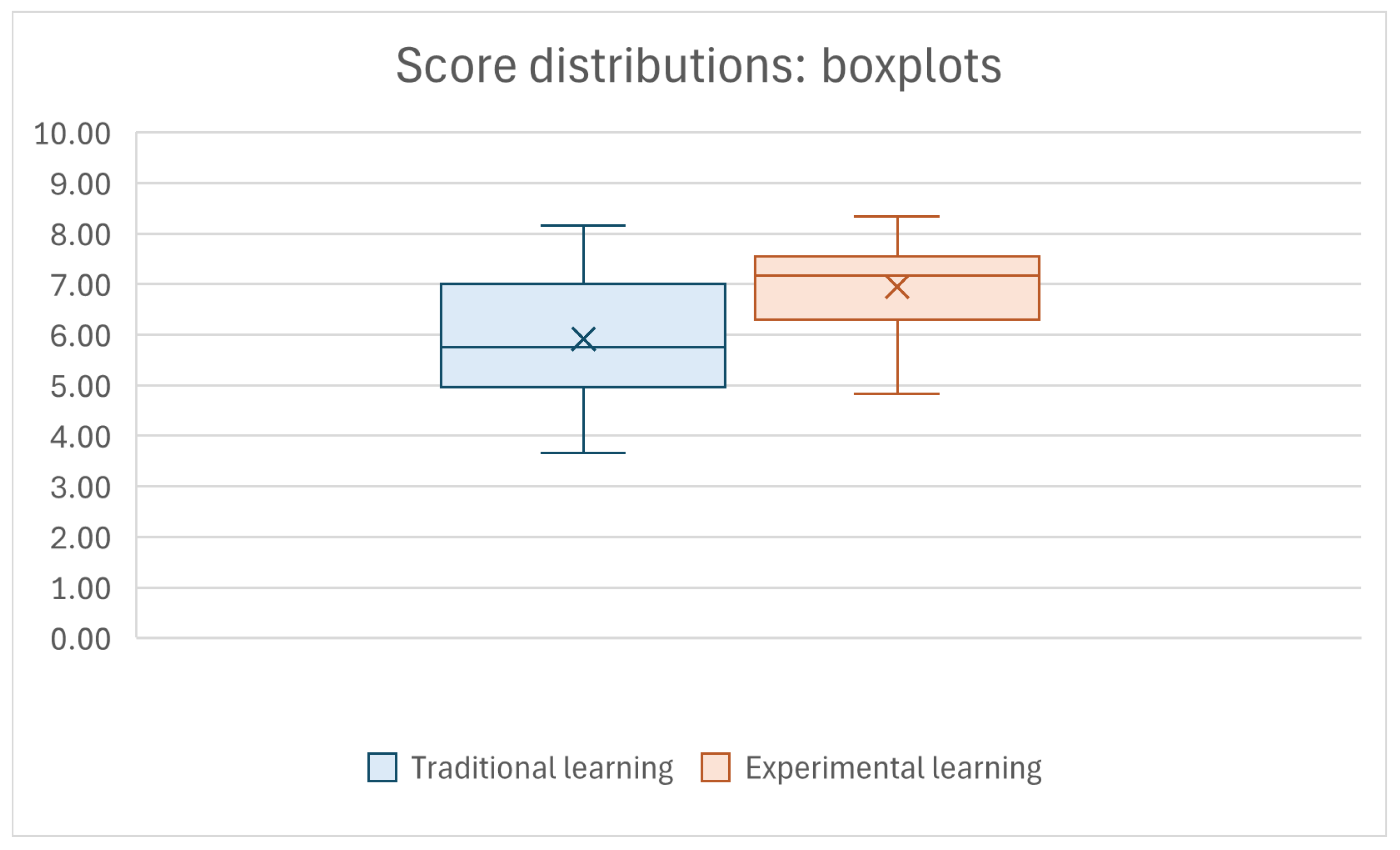
In order to better compare the academic performance obtained in both courses, visual representations have been added to clarify data distributions and trends. Specifically, a boxplot and a barchart have been designed, where the metric chosen in both cases has been the distribution of average scores overall per student for each course.
In this sense,
Figure 2 shows the boxplot obtained out of each distribution made up with the average score overall per student obtained last year with a traditional learning paradigm and this year with an experimental learning paradigm. The former is colored in blue and it is located on the left hand side of the
x axis, whereas the latter is colored in orange and it is located on the right hand side of the
x axis. On the other hand, the vertical axis shows the range between 0 to 10, which are the bottom and top scores in the Spanish grading system, respectively.
The interpretation of a generic boxplot goes as follows: the lower edge of the box is the first quartile (Q1), whereas the upper edge is the third quartile (Q3). The middle line within the box accounts for the second quartile (Q2), also known as median, whilst the cross inside the box is the mean. The height of the box accounts for the interquartile range (IQR), while the lower line outside the box is the value Q1 − 1.5·IQR, whilst the upper line outside the box is the value Q3 + 1.5·IQR. Any value below the former line or above the latter line is considered an outlier and it should be detected and treated accordingly. Sticking to a normal distribution, and specifically to its probability density, IQR area covers the half of the values (50%) in the distribution, whereas the area from Q1 to Q1 − 1.5·IQR covers nearly a quarter of the values (24.65%), and so does the area from Q3 to Q3 + 1.5·IQR, while the values beyond those boundaries are considered outliers, where 0.35% is assigned to the far lower area and also to the far upper area.
Focusing on the boxplots shown herein with the score distributions of both years, the one corresponding to traditional learning exhibits a higher IQR, which means that the average scores overall per student are more widespread, whereas the median is closer to Q1, with the mean being slightly higher. On the other hand, the one corresponding to experimental learning depicts a smaller IQR, thus meaning that the scores are tighter, whilst the median is closer to Q3, with the mean being slightly lower. Comparing both boxplots, it is clear that the score distribution out of the experimental course presents significantly higher marks with respect to the traditional course. Moreover, the experimental course displays a higher mean and lower variability than the traditional course.
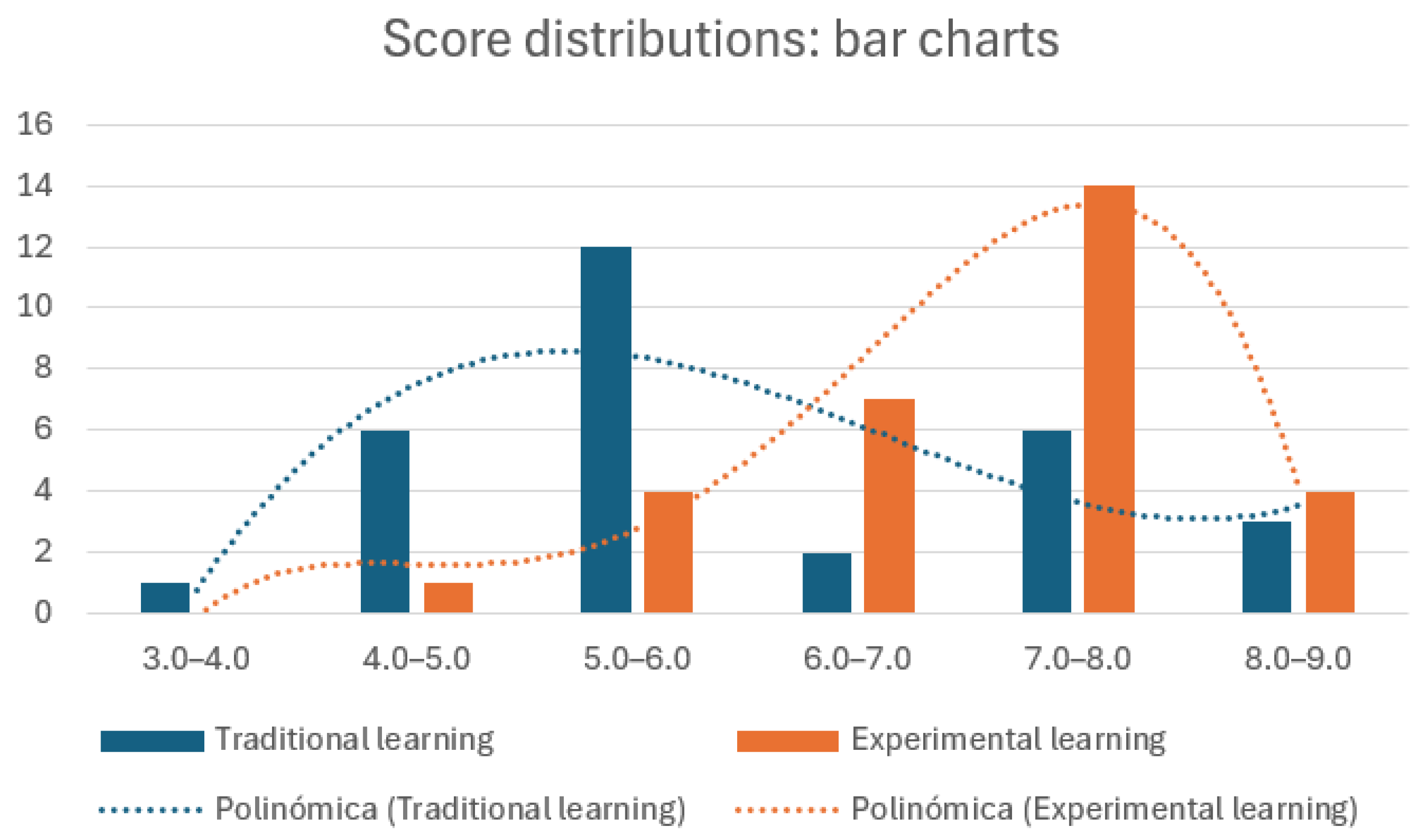
Analogously,
Figure 3 shows the barcharts obtained out of each distribution for the average score overall per student, where the same color codes as above has been used. The
x axis has been organized in intervals of one point, starting with a natural number and finishing right on the limit of the subsequent natural number, whereas the
y axis shows the frequency of instances within each of those intervals, as the scores obtained are continuous values. Only the intervals with some instance have been drawn in order to obtain a clearer picture.
Focusing on the barcharts shown herein with the score distributions of both years, it is easy to see that the bars representing the traditional course are higher on lower intervals, namely those located on the left, whilst the bars standing for the experimental course are higher on higher intervals, namely those located on the right. This point shows the improvement achieved with the new paradigm with respect to the old one according to the metric considered herein, which is the average score overall per student.
Additionally, polynomial tendency lines have been drawn for the bars corresponding to each learning paradigm, where the color coding has been maintained. Looking at the one standing for the traditional course, the polynomial tendency line increases quickly up to the interval between 5 and 6, and from that point on, it decreases slowly. However, the polynomial tendency line for the experimental course increases steadily up to the interval between 7 and 8, and then it decreases sharply. Comparing both barcharts and both tendency lines, it is clear that the score distribution from the experimental course presents significantly greater grades with regards to the traditional course.
Table 5 depicts the success rate attained in both courses, which was calculated as the rate of students who passed a course with respect to the overall students attending that course, and considering that the passing grade under the Spanish grading system is 5 out of 10. An increment of over 16% was experienced in the present academic year compared to the previous one. As stated for the academic performance, this may induce the idea that learners obtained extra motivation due to the new course setup, which led them to attain a higher success rate. Moreover, this percentage of increase in success rate is close to the 20% increase stated in the literature for the application of an active learning paradigm in STEM-related courses (
Nurbavliyev et al., 2022). As stated above, this experimental course was not thought to be strictly within the active learning paradigm, although group activities were run during the sessions so as to furnish students with a more active role.
Table 6 exhibits the skewness and kurtosis for each teaching unit and for the average score overall. It should be remembered that skewness is a measure of the symmetry in a data distribution, whereas kurtosis is a measure of the relative size of the tails in a data distribution. According to the values obtained, the assumption of normality was established for the data collected in both years because all variables in this table are located within the range going from −2 to +2, which indicates the normality of the data collected (
Moghadamnia & Soleimani-Farsani, 2023). This way, the normality assumption states that such data follow a normal distribution. This is equivalent to say that the sampling distribution of the mean is normal, or otherwise, the distribution of means across samples is normal.
Table 7 shows the most common dispersion statistics related to the marks obtained in both academic years. With respect to the variance, there was a reduction of around 25% in the current academic year, whilst the standard deviation was reduced by around 13%, whereas the coefficient of variation reduced by around 10%. Hence, it happens that all three measurements decreased in the current academic year, which implies that most of the marks obtained were closer to the average values in a pretty remarkable manner (
Roig et al., 2024b). On the other hand, the marks obtained in the last academic year were more spread out.
Table 8 exhibits the Cronbach’s Alpha achieved with the marks achieved in both courses. The value obtained in the previous academic year was a bit under 0.8, which is the threshold of a good reliability. On the other hand, the value attained in the present academic year was 0.704, which is on the verge of the threshold of an acceptable reliability. Hence, a decrease of around 10% was experience in the marks of the current academic year, which means that the correlation among the marks obtained was lower compared to the case in the previous academic year. It should be noted that Cronbach’s Alpha is related to reliability and internal consistency of data, as well as with the correlation degree (
Taber, 2018). Therefore, the results achieved in both courses can be considered reliable.
Table 9 summarizes the relevant measurements obtained with centralization statistics in order to apply inferential statistics. Those measurements are the count of students in each course, which happened to be the same, the average of the marks obtained in each course, which is referred to as the mean, and the standard deviation of the marks attained in each course (
Roig et al., 2024c).
Table 10 exhibits the result of the
T-test applied to the distribution of marks obtained in the previous and the current academic year. The value obtained according to the
T-student distribution table was 2.045. Also, the degrees of freedom in this scenario were 58, because the number of students in both courses were 30 + 30 = 60. With both values, the calculation of the
p-value yielded 0.017. This value was lower than the
s-value established, which was 0.05, hence the interpretation of this
p-value was that the improvement of the results achieved in the current academic year was statistically significant compared to those achieved in the previous academic year.
Table 11 depicts the calculation of the Cohen’s
d in order to quantify the effect size, which could be seen as the magnitude of the difference between both distribution of marks (
Sullivan & Feinn, 2012). The value achieved for Cohen’s
d is 0.637, which is located within the interval going from 0.50 to 0.80. The values within this range are considered between a medium effect and a large effect. In order to define those effects, it must be considered that a small effect is noticeably smaller than medium, although it is not that small to be trivial, then, a medium effect is likely to be visible for a careful observer with the naked eye, and in turn, a large effect is as far away above the medium as the small is below it (
Brydges, 2019). Hence, in this case the effect size can be considered quite noticeable.
At this point, before getting to the results for sample size, it should be noted that hypothesis testing considers two different situations when comparing two distributions, such as the null hypothesis and the alternative hypothesis. The former claims that the values being compared are equivalent, which is often referred to as : , where and stand for the mean of the first and the second distribution, respectively. On the other hand, the latter claims that values being compared are not equivalent, which is often referred to as : .
Furthermore, any decision about hypotheses may incur a certain degree of error, where the most relevant ones are Type-I error and Type-II error. The former is also known as false positive, which is the probability of rejecting the null hypothesis in case it should not be rejected. The most common accepted value for Type-I errors is
, although
is sometimes used, and this rate is considered the significance level. On the other hand, the latter is also known as false negative, which accounts for the probability of failing to reject the null hypothesis in case it should be rejected. The most common accepted value for Type-II errors is
, although
and
are sometimes used (
Cohen, 1992).
Additionally, the rate ranges from 0 to 1, which is the same case as with . However, has an inverse relationship with another variable called statistical power, which in turn is calculated as , thus ranging from 0 to 1 as well. Therefore, power could be defined as the probability of correctly rejecting the null hypothesis if a fixed effect size and a fixed sample size are considered. In other words, power could be seen as the probability of correctly detecting an effect if there is indeed a real effect to detect. Hence, the higher the power, the better the results obtained, even though is the most common value in the literature, leading to .
The sample size is related with the effect size, power, and alpha, such that knowing three of those values, it is possible to calculate the other one. In this sense, if
and power, or its inverse value
, are known, then the appropriate sample size could be found out in order to achieve a given effect size, or otherwise, the smallest effect size to be reliably detected could be found out for a given sample size (
Serdar et al., 2020).
Taking all this into account,
Table 12 displays the sample size required to obtain the desired effect size. Actually, the first row shows the sample size for the effect size achieved, which is 0.64 (rounding up to two decimal digits). Then, two more rows are included as references, where the second row considers an effect size of 0.50, which is the lower bound of the interval where the effect size achieved is in, and the third row takes an effect size of 0.80, which is the upper bound of the interval. Additionally, the values of
and
have been fixed in all these calculations to 0.05 and 0.20, respectively.
The sample size values could be found out by different means, such as applying a specific expression related to the inverse of the normal distribution, or searching the values in a specific table, or even applying Lehr’s rule of thumb, which gives good approximations when and . In any case, the sample size for an effect size of 0.64 is 39, whereas the sample size for an effect size of 0.50 is 63, whilst the sample size for an effect size of 0.80 is 25.
On a regular basis, the smaller the effect size desired, the higher the number of participants needed, considering and . In addition, the sample size obtained is the ’ideal’ size, such that a lower amount of participants do not allow us to detect the effect size desired, whereas a higher amount of participants are unnecessary to detect the effect size desired. In this case, as the number of students in each distribution is 30, and the sample size calculated for the effect size achieved is 39, then it can be concluded that the number of participants was not sufficient to detect the effect size of 0.64, although the results achieved were relatively close to it. Hence, further research should be undertaken in the future with larger groups.
On the other hand, no structured interviews were held with students about the format and the content of the experimental course. However, comments made by students during the course were collected and dealt with. To start with, the difficulty getting used to hybrid sessions was one of the most repeated comments in the first stages due to the novelty for the students. Luckily, this kind of comment disappeared in a few sessions, as happened with the other types of negative comments. Another common issue was about the technical requirements needed, as some students had a hard time getting connected and interacting through the LMS during the initial sessions.
Further comments were received about having the course settings constantly changing, as some students found it tough to change the settings so often, although those sorts of comments stopped after some sessions, as students got used to it. Another sort of comment was about the lack of socialization and peer support, but this type of comment stopped at some point, as chats and forums were available for communication among instructors and peers. Finally, another kind of comment was about the difficulty to follow sessions in foreign language due to the lack of proficiency in English, but such comments were no longer received after some sessions. Nonetheless, most students assessed this experimental course in a positive manner.
6. Conclusions
In this paper, a study about combining space, time, and language in active learning scenarios has been described. To start with, those features have been considered in different ways in the literature, although they have been redefined in this work in the following way: space for the physical location where the learning process takes place, time for the moment when the learning process takes place, and language as how the learning process is driven.
Three values have been established for each of those three features, where the value 0 is the traditional option, the value 1 is the innovative option, and the value 2 is the hybrid option, where the other options are mixed together. This way, regardless of the particular feature, option 0 is the easiest one to be implemented, option 1 requires some extra effort to get it running, and option 2 implies a much higher effort in order to keep up with both at a time.
The combination of all three values for all three features leads to an overall amount of 27 possible combinations available, each one with its own benefits for the learning process, as well as with its own drawbacks when it comes to effective deployment. Moreover, it should be noted that the ideal situation would be to be able to adjust any of the values within a triplet for a given lesson by just changing some setting in the LMS being used, which would give absolute freedom in order to deliver a particular lesson.
However, in order to implement many of those combinations, there are some prerequisites. The first one is the acquisition of the appropriate audio equipment with enough quality so as to achieve a high definition transmission of the sound for all users. Likewise, the second one is the acquisition of the proper video equipment with enough quality so as to obtain a high definition transmission of the video for all users. Finally, the third one is the acquisition of a computer-aided translation system in order to carry out automatic translations between languages, even though this step may not be needed if all attendants are fluent enough in both languages involved.
Additionally, this framework was implemented in a computer science course in the current academic year, which allowed us to compare the results obtained with those achieved in the previous academic year with a traditional learning scenario. Results showed an increase in academic performance, as well as in success rate. On the other hand, the difference in the results were statistically significant, although the calculation of the sample size led to the conclusion that the number of participants were not sufficient to detect the effect size desired.
Regarding the potential limiting factors affecting this study, it seems clear that teachers, students, and administrative staff had to apply extra effort during the experimental course compared to their efforts in the traditional course, mostly in the first sessions, due to the novelty of the paradigm. Nonetheless, it should be considered that the same teachers taught both courses, whilst the participants in both courses are college students with no specific particularities, whereas administration staff was the same during both courses and the software applications used in the latter course were already installed in the former course, even though they were obviously massively used during the latter course. Hence, it could be said that neither of those three type of issues could be considered an actual limiting factor.
With respect to sample size, the same number of students took part in both courses, where all students took part in the study. Hence, it was not possible to include more students in this particular study in any of both academic years. The calculation of the minimum sample size to detect the effect size achieved in this study showed that the amount of students was not sufficient, provided the statistical power and the statistical significance took the most common values. Therefore, the number of participants could be seen as a limiting factor, even though it could not be sorted out, as no more students were available in this study.
With regards to confounding variables, the environment where both courses were held was different, which led to multiple differences in the way each course was faced by the students. According to the comments of students received during the experimental course, students faced some difficulties at the beginning of such a course due to the novelty. To start with, the difficulty to adapt to hybrid sessions was a quite common comment in the first stages. Another common issue was related to the technical requirements needed in the experimental course, which was a handicap to some students during the initial sessions.
Besides, the constant change in the settings of the course was tough, until students got used to it. Moreover, the lack of socialization was pointed out compared to traditional courses. Also, the lack of proficient skills in the foreign language was also indicated, which refrained some students from properly following those sessions. Those could be considered limiting factors, even though most students were able to overcome them as the sessions went by. However, in spite of those limiting factors, most students positively assessed the experimental course.


