Article

High School Students’ Performances in Transitions between Different Representations of Linear Relationships in Mathematics and Physics

Department of Physics E. Pancini, University Federico II, 80143 Naples, Italy
*
Author to whom correspondence should be addressed.
Educ. Sci. 2022, 12(11), 776; https://doi.org/10.3390/educsci12110776
Submission received: 27 September 2022 / Revised: 24 October 2022 / Accepted: 27 October 2022 / Published: 1 November 2022
(This article belongs to the Special Issue Innovation in Teaching Science and Student Learning Analytics)

Abstract

:
This study involved 643 high school students to assess their performance in using different representations of linear functions—graphs, tables, and algebraic relationships—in mathematics and kinematics. The results show that students encounter greater difficulties when they have to interpret representations involving algebraic relations in mathematics. Furthermore, it is shown how the ability to switch from one type of representation to another is influenced by spatial reasoning skills, orientation toward physics, and self-confidence in the field of mathematics and physics. Implications for teaching kinematics and linear functions are briefly discussed.

1. Introduction

The OECD PISA (Program for International Student Assessment for the 2018 report (see [1]) studies in recent years have revealed widespread difficulty for Italian pupils in science and mathematics. These difficulties have serious consequences on the scientific education of students, who will be increasingly required to participate in the public debate on issues involving scientific topics as informed citizens [2]. Although several measures have been implemented locally over the past years to improve this situation, a coherent framework does not yet seem to emerge that can help in describing, interpreting, and overcoming students’ difficulties on basic topics in mathematics and science, and in physics in particular. In this article, we will focus on how high school students (10th grade) interpret linear functions in the context of linear functions and in one-dimensional (1-d) kinematics (uniform rectilinear motions). In particular, we will analyze the students’ ability to represent a linear function or a motion using different forms of representation: the objects of our research will be graphs, tables, and algebraic formulas.
The choice of kinematics as the area of our study is justified by the massive use in this field of different types of representations (graphs, equations, tables) and by the presence of known misconceptions that influence the understanding of the representations of motions. The choice of linear functions is due to the fact that, although this topic is targeted both in the middle and high school math syllabi, the PISA tests’ data show persistent difficulties of students in obtaining information from written texts and diagrams. Considering the definition of mathematics literacy given by PISA in [1], namely the “students’ capacity to formulate, employ and interpret mathematics in a variety of contexts, including reasoning mathematically and using mathematical concepts, procedures, facts and tools to describe, explain and predict phenomena”, we chose to focus this research on the ability to obtain information from a specific representation, consequently identifying the same information in a different type of representation.
The didactic context chosen for this research consists entirely of a large audience of students from technical and professional institutes in a large city in the South of Italy. This choice responds to the need to investigate the difficulties encountered in the physical and mathematical field of a sample that national and international surveys indicate to be consistently below the average performance in the age group of 14–15 years. To understand possible reasons for these difficulties, in addition to the ability to solve the proposed exercises on linear functions and 1-d kinematics, we investigated the students’ ability in spatial reasoning, confidence in the answers given, and perceived orientation toward physics in math and physics, to show if and how cognitive and metacognitive variables affect the students’ performance.
In the next section, we will briefly review the results obtained so far in the research in physics education regarding the students’ difficulties in kinematics concepts (e.g., velocity), the related mathematical concepts (e.g., slope), and the typical representations (e.g., graphs). In the second, third, and fourth sections, we present the methods of analysis, the measuring instruments, and the results, respectively. In the concluding section, we will discuss the possible didactic implications of this study.

2. Theoretical Framework

2.1. Students’ Difficulties in Kinematics

As mentioned above, kinematics is one of the fields of physics in which several studies have been conducted on students’ ideas since the 1970s [3,4,5,6,7]. One of the most common misconceptions of students that emerges from these studies is to consider the graph of a law of motion as a photograph of motion itself [5]. This can happen because, to imagine how a phenomenon that occurs as time changes is graphically represented, and to interpret it correctly, it is necessary to resort to the abstract idea of function. This difficulty can also be due to a lack of attention that students show in reading the variables on the axes of the graphs. Another common misconception that emerges from the interpretation of distance-time graphs by the students is the so-called “point-interval confusion” [8]: from the interviews with the students carried out in this research, it is evident that, in their reasoning, they often do not distinguish an instant from an interval of time; this implies, for example, not being able to distinguish the concepts of average speed and instantaneous speed. This difficulty emerges only in a purely physics context and it is different from not being able to interpret the limit of the incremental ratio, through which the instantaneous speed is defined. Understanding the concept of instantaneous velocity would also help to clarify what is meant by the initial velocity of a motion. In the kinematic description, the initial velocity is a characteristic of motion for its entire duration. However, this physical dimension does not often appear in the reasoning of students, which instead includes naïve concepts such as that of “initial push” or “force in the direction of motion” [9], which would “wear out” in some way during motion. This shows how the same students, ignoring or not having understood the first principle of dynamics, interpret the initial dimension of motion as a force and not as a velocity. This probably happens because the students imagine a real situation, where the presence of friction implies that in order to have an object in motion it is necessary to apply a force on it. Furthermore, students do not always exactly know the vectorial relationship between speed variations and applied forces. For example, in the same study [9], most students think that an object dragged by another one along a given direction, when released, does not gain speed in that direction.
Another specific difficulty in kinematics is the one that many students show in dealing with negative speeds [3]. A first observation should be made on the used terms, as in the Italian language, unlike for example the English one, the same word is used to indicate both the module of the vector and one of its components along a given direction. In this way, students do often not recognize negative speed or misinterpret it. Furthermore, students also have difficulties in interpreting the negative component of a vector, which requires, even in a very simple case such as the one-dimensional one, the operation of projection of a vector along an axis.
In the analysis of misconceptions relating to kinematics, as evidenced by more recent research studies [10,11,12], a problem of knowledge transfer emerges between the context of mathematics and that of physics. In fact, it is now commonly accepted that mathematical knowledge and skills are necessary but not sufficient for solving problems in physics. Often, however, it is not enough to have only physical knowledge, it is also necessary to know how to connect the two fields. Regarding this aspect, it should be noted that, for example, the difficulties related to the concept of negative velocity overlap with the greater difficulty that students often present in understanding the decreasing functions. As a further example, other studies report that knowing how to determine the slope in a y-x graph and knowing how to qualitatively interpret distance-time graphs is not always sufficient to determine the speed in a graph [13]. For these reasons, it can be useful to study students’ specific difficulties with mathematical entities such as graphs.

2.2. Students’ Difficulties with Graphs

Much research has highlighted students’ difficulties in understanding and use of mathematical entities (such as graphs) widely used in the kinematic field. For instance, the concept of slope [11], is often confused with the altitude at which a point is found on the curve of the graph representing the law of motion, even though this misconception disappears with increasing age. Other students, on the other hand, identify the slope of a line as the angle between the line itself and the abscissa axis. This idea may be due to the confusion between angle and area; in this case, the error would in fact also be not considering the slope as a dimensionless quantity. Furthermore, the slope is confused with the intercept value at the origin, or students think that the slope sign depends on the quadrants in which the line is drawn. This also reveals the fact that some students are influenced by how the line is represented in the quadrants of a Cartesian plane, for example, if it passes from one quadrant to another, not being aware of its infinity extension on both sides. Finally, some students swap the numerator and denominator in the definition of slope. However, although they do not have a precise idea of the concept of slope, many students often manage to solve qualitative questions about it, as it remains a term that is part of the common language. On the other hand, the use of the word “slope” in common language could also generate problems: for example, some students may find difficulty when dealing with negative slopes. This difficulty, in addition to the difficulties related to the concept of negative numbers highlighted in many areas, could also reflect the fact that in the common language the slope is a definite positive, and it is often expressed in percentage terms (such as in road signs).
The process of understanding graphs can be interpreted on the base of the Carpenter and Shah model [8,11], which includes a sequence that integrates perceptual and conceptual aspects. The former refers to the recognition of patterns, such as decoding and interpreting the positive or negative slope and the types of curves represented; the latter refers to the qualitative and quantitative interpretation of the observed models, such as those regarding the labels and axes scales, or the units of measure).

2.3. Students’ Difficulties with Other Representative Formats

The modality with which motions are often represented in kinematics is not limited to Cartesian graphs. Also, functions in mathematics are represented with graphical and textual modalities. In the literature, various examples of interaction effects of the representation format with the type of functions to be studied are reported [13]. In particular, the type of modality used to describe a certain phenomenon significantly influences both the test results and the resolution strategies adopted (especially in the field of kinematics). It has been found, for example, that a certain modality can facilitate the study of a given function and, at the same time, can make that of another function more difficult. In particular, students perform worse on linear functions when they are represented by means of formulas rather than tables. Another interesting result obtained in [13] concerns the fact that by allowing students to choose the modality of representation of the question, the number of correct answers increases for some individuals, while for others it decreases. The mentioned study also highlights the existence of a relationship between the age of the students and their preferred representation format; in particular, the choice of formulas increases with age, but this does not imply that fewer errors are made in this way than using other representations. This choice could in fact depend exclusively on the more frequent use of formulas compared to graphs and tables in traditional teaching, due to their conciseness.
To address these difficulties, students should become aware of how the same phenomenon can be described using different representations. In this study, we focus on the so-called “representational fluency”, defined as “the ability to interpret and construct representations, and to know how to pass from one to the other” [13], limiting our attention to the case of the linear functions. The ability to switch between different representations is a key aspect of acquiring problem-solving skills [13]. The authors also show that, for different types of functions (for example, direct and inverse proportionality), students perform better in the transitions between graphs and tables, while they show greater difficulties in the transition between formulas and graphs and between graphs and formulas. However, the authors note that a secondary interaction effect between the type of representation and the type of function can affect students’ performance.

2.4. Metacognitive Skills Relating to the Interpretation of Representations

Given that the ability to switch between different modalities depends on the starting representation (table, graph, and formula in increasing order of difficulty), a possible interpretation is that students’ difficulties in correctly answering questions with different representations of the same phenomenon may be due to an erroneous perception of their ability to interpret one type of representation compared to another. Therefore, to investigate the effect of this perception, it may be useful to study the level of self-confidence in the response given to a specific problem. The assessment of one’s own understanding is defined as “the aspect of thinking regarding one’s own reasoning” [14]. A correct self-judgment is a prerequisite that would allow students to regulate their learning, recognizing the aspects they need to improve on. Research in educational psychology has found evidence of the so-called Dunning–Kruger effect, according to which, generally, individuals who lack content knowledge also lack metacognitive abilities; because of this, the students with the worst results tend to overestimate their knowledge (overconfidence bias), while those with the best results are generally more accurate in this judgment. Other studies [13] have also shown that in some cases students who obtain better results cannot clearly distinguish the items they are able to answer from those they are unable to answer, thus demonstrating a not complete understanding of the concepts under investigation.
Another construct that can influence the ability to correctly interpret different types of representations is the “orientation toward physics” that, based on a validated instrument, measure grouping the literature on metacognition about information’s elaboration in the learning process, self-efficacy (related to Bandura’s framework, see [15]), self-regulation in study activities, engagement in learning and anxiety management [16]. These dimensions are highly correlated and may significantly impact students’ achievements during their school careers [16].
For both of these constructs, previous results indicate a significant gender difference.

2.5. Spatial Reasoning Skills

Another important factor that can potentially influence the understanding of the representations of motions (especially in the extrapolation of information from graphs) is the spatial ability, defined as “the ability to generate, store, retrieve and transform well-structured visual images” [9,12,17]. The differences between individuals in spatial ability have been studied since the 1920s when psychometric research demonstrated the difference between this ability from verbal and numerical ones. In [9], an example of research is reported concerning the study of the relationship between the resolution of different types of problems in physics and spatial ability. The results show that physicists show a high level of spatial ability, to a greater extent than students of non-scientific subjects. This evidence indirectly shows that this ability is a component of intelligence relevant to problem-solving. Furthermore, the authors show that the description of the trajectory of an object using vectors and the inference of the characteristics of a motion starting from its description in another reference system can be linked to spatial ability, while the typical problems of one-dimensional kinematics are mostly related to the ability to manipulate equations.
Furthermore, some research has shown that for students with low spatial skills, some misconceptions related to one-dimensional motions are more resistant, such as the interpretation of the graph representing the law of motion as a photograph of the motion itself [9]. Therefore, it is possible that students with high spatial ability, through their daily experience of motions, have developed more sophisticated ways of analyzing them, helping them in understanding concepts. Overall, such evidence suggests that the correct interpretation of graphs can be a direct or indirect consequence of a high level of spatial ability.
Finally, recent studies on eye tracking have also shown a correlation between spatial ability and eye fixation on the area of interest of the motion [11], as well as with the ability to solve problems correctly. Using as an interpretative framework the model of Carpenter and Shah, these studies show how individuals who have correctly identified the trajectory of a motion move their eyes on the directions of both axes, suggesting that they are integrating the two directions of motion, while those who answer erroneously often neglect the horizontal component on a visual level. Instead, students with high and low spatial ability spend the same time studying the curves represented, suggesting that both groups focus equally on interpreting the visual representation. Furthermore, students use the time variable in the same way to interpret motion under consideration, regardless of their spatial ability. Instead, the actual axes are studied more by students with high spatial ability, who often give a specific description of what happens interval by interval, highlighting the changes in the characteristics of the motion. The study of axes and labels is therefore consistently repeated several times by students with high spatial ability (“iteration of Carpenter and Shah”). In this study, we will focus on a specific aspect of spatial ability, the mental rotation, that is, the ability to imagine the possible rotations of three-dimensional objects [12,18]. To measure this ability, we will use the Mental Rotation Test (see [18]), in which the emphasis is also placed on the speed of resolution. The previous results indicate a significant gender difference for this ability too.

2.6. Research Questions

Based on the literature discussed above, the main research questions in this study are:
(RQ1) How does representational fluency differ between mathematics and physics?
(RQ2) How does the representational fluency differ between the different types of linear functions?
(RQ3) What is the influence of self-confidence, orientation toward physics, spatial ability, and gender on representational fluency in mathematics and physics?

3. Materials and Methods

3.1. Instruments

In this study, we used several instruments. They are reported in Appendix A (in English language, but they were submitted in Italian language), following this subdivision:
  • A kinematics test, concerning the laws of uniform rectilinear motions, composed of twenty multiple choice questions divided into three groups (respectively of six, eight, and six questions). The groups are characterized by a specific representation of the law of motion (table, graph, or algebraic relation). It is required to identify the other two corresponding representations, among six possibilities: these correspond to six types of linear functions, which are obtained by combinations of the sign of the angular coefficient and the intercept value at the origin, as described below.
  • A mathematics test, concerning linear functions, with the same structure as the physics test.
In these two tests, we used three types of representations: R = algebraic relation, G = graph, T = table. Consequently, we have six possible transitions, and they will be indicated in the following ways: GT, GR, RG, RT, TG, TR, where the first letter indicates the initial representation and the second the corresponding one that students are asked to identify. Regarding the classification of linear functions, we will characterize the questions according to the following notation: PP, PZ, PN, NP, NZ, NN, where the first letter indicates the sign of the angular coefficient and the second that of the intercept value at the origin (the letters P, Z, and N represent respectively positive, null, and negative values). The two contexts, mathematics and physics, differ slightly in the number of questions per type of function.
In drafting the two tests, attention was paid to some details in order to facilitate the exercises’ solution. For instance, in the graphs of the laws of motion, only the first and fourth quadrants are shown to make evident the start of motion in the origin of the time axis, while in the mathematics section a small section of the second and third quadrants is reported to show that the domain of the function is given by the whole real axis. In addition, no numerical values other than the origin are shown on the axes, to avoid the use of numbers when not necessary, with any calculation errors. Furthermore, all tables show the same values of the independent variable: 0, 1, 2, 3, and 4. In fact, the use of integer and equidistant numbers facilitates the deduction of the slope, if the student is mnemonically induced to apply the analytical formula for its calculation. In particular, for functions with negative origin intercept, the tables show only negative values of the dependent variable.
The possibility to directly compare the results obtained by students in responding to the kinematics and mathematics items is guaranteed by the fact that both require the same procedures for the resolution: the student should recognize the sign of the two parameters that characterize the line, finding the two corresponding representations consequently. Thus, it is not necessary to know any formula for the explicit calculation of the values of these quantities (which, however, could only be carried out starting from the tables’ values).
  • A questionnaire about self-confidence in which students are asked to express, for each group of physics and mathematics questions, the level of confidence in the answer given. This is done through a linear measurement scale (Likert scale) ranging from one (“not at all”) to five (“totally”).
  • A questionnaire about the orientation toward physics, specifically developed for this study on the basis of literature, consisting of 30 statements for which the student must indicate their level of agreement, on a scale from one (“not at all”) to five (“completely”). The questionnaire is reported in the appendix.
  • The Mental Rotation Test (MRT) (see [18]). It consists of 20 multiple choice questions in which the respondent is asked to indicate out of four three-dimensional figures proposed, which correspond to a correct rotation of the figure present in the frame. Each question presents two correct and two wrong alternatives; the wrong ones correspond to a reflection of the figure itself and to a rotation of the figure present in another question. Usually, a restrictive evaluative criterion is used, considering only the answers with both correct alternatives as the correct ones.
Students had 45 min to complete the test, divided into three parts of 15 min each.

3.2. Sample

The sample of the research was made up of 643 high school students, whose age was between 14 and 15 years old. The percentage of girls in the sample was about 33% (N = 214). The participants were from seven different schools in a large city in the South of Italy, attending the second year of their high school course. All students attend the same type of study course, mainly focused on technical subjects and little on physics, thus constituting a homogeneous sample.
The classes, through their teachers, have been involved in the study voluntarily, having given their consent to take part in the research.
All the following steps of the data analysis were carried out by means of the SPSS statistics package.

3.3. Reliability

In Table 1 the values of the McDonald’s Omega index for each of the instruments are reported. All reliability values are satisfactory (McDonald’s Omega > 0.8), so the following results can be considered representative of the population under investigation.
Data imputation techniques were implemented to replace blank answers, in the following way: for the instruments characterized by the dichotomy in correct/wrong answers (physics, mathematics, and MRT) all cases corresponding to no answer given were considered incorrect. For instruments characterized by responses on a Likert scale (self-confidence and orientation toward physics), we used the median value of the group of participants coming from the same school, for the corresponding item.

3.4. Scoring of Tests on Kinematics and Mathematics

The analysis of the tests was carried out by assigning 0 points to the wrong answers and 1 point to the correct ones. Initially, the overall performance of the two tests was assessed through the total score, obtained by adding those of the individual questions. Subsequently, average scores were calculated on the groups of questions sharing the same type of transition or function, separately for the two contexts, kinematics and mathematics. A paired-sample t-test was performed to observe the difference between the scores in physics and mathematics on these groups of questions. Then, exploratory factor analysis was carried out, taking into account both the kinematics and mathematics tests, in order to identify any common latent dimensions relating to the interpretation of representation modalities in mathematics and physics. The “parallel analysis” method was used to choose the number of optimal factors, namely comparing the results obtained with those generated by a random matrix. The McDonald’s Omega was then recalculated for each of the latent factors found, to assess their reliability.

3.5. Confidence Bias

Average confidence scores were first calculated separately for the two contexts for the groups of questions that share the same starting representation (e.g., a table, a graph, a formula). Then we normalized the obtained scores (values between +0.2 and +1) and subtracted the normalized average scores of the corresponding group of knowledge questions (values between 0 and +1), obtaining an estimate of the accuracy of self-evaluation. Note that, in this way, the range of possible values for the accuracy of self-evaluation varies between −0.8 to +1. Due to the normalization of the confidence scale, values of accuracy of self-evaluation between 0 and +0.2 indicate that the student is averagely calibrated. Values between +0.2 and +0.4 indicate moderate overconfidence bias, while values greater than +0.4 indicate significant overconfidence bias. Negative values indicate under-confidence bias. Then, the average accuracy of self-evaluation scores was calculated and a paired-sample t-test was performed to study the differences between the physical and mathematical contexts, as well as the gender differences.

3.6. Factor Analysis of the Orientation toward Physics Questionnaire

Since we used a newly developed instrument, exploratory factor analysis was carried out on the orientation toward physics items, using the criterion of the inflection point in the eigenvalue graph to choose the number of latent dimensions to be considered. Items with loadings lower than 0.4 were not included in the final solution. Then, McDonald’s Omega was recalculated for each factor. Subsequently, the average scores for the obtained factors were calculated, and a paired-sample t-test was performed to evaluate the significance of the difference between these dimensions for the two contexts (kinematics and mathematics). Finally, gender differences for each dimension were assessed.

3.7. Scoring of the Mental Rotation Test

We assigned a score of 0 to wrong answers and 1 to correct ones of the Mental Rotation Test (MRT). For each participant, an average score was calculated, and gender differences were evaluated.

3.8. Linear Regression

Multiple linear regression analysis was carried out to investigate the influence of confidence, orientation toward physics, spatial ability, and gender on the mean scores obtained on the average score in the kinematics and mathematics knowledge questions, respectively, and on each of the latent factors found through exploratory factor analysis. The generic equation of linear regression is:
Yquest = α + β1XSC_K + β2XSC_M + β3XOTP + β4XSP + β5XG + ε
where: Yquest is the normalized average score obtained on the kinematics and mathematics tests, and on each of the latent factors; α is a coefficient that estimates the constant effects not due to the independent variables; XSC is the average normalized self-confidence score in kinematics and mathematics; XOTP is the average normalized score for each of the factors of the orientation toward physics scale; XSP is the average normalized score for spatial ability; XG is the gender variable (coded as 0 for males and 1 for females); ε is the estimate of the regression error; βi are the estimates of the normalized regression coefficients. The regression was carried out by means of the SPSS statistics package, following the “backward” method.

4. Results

4.1. Tests on Kinematics and Mathematics

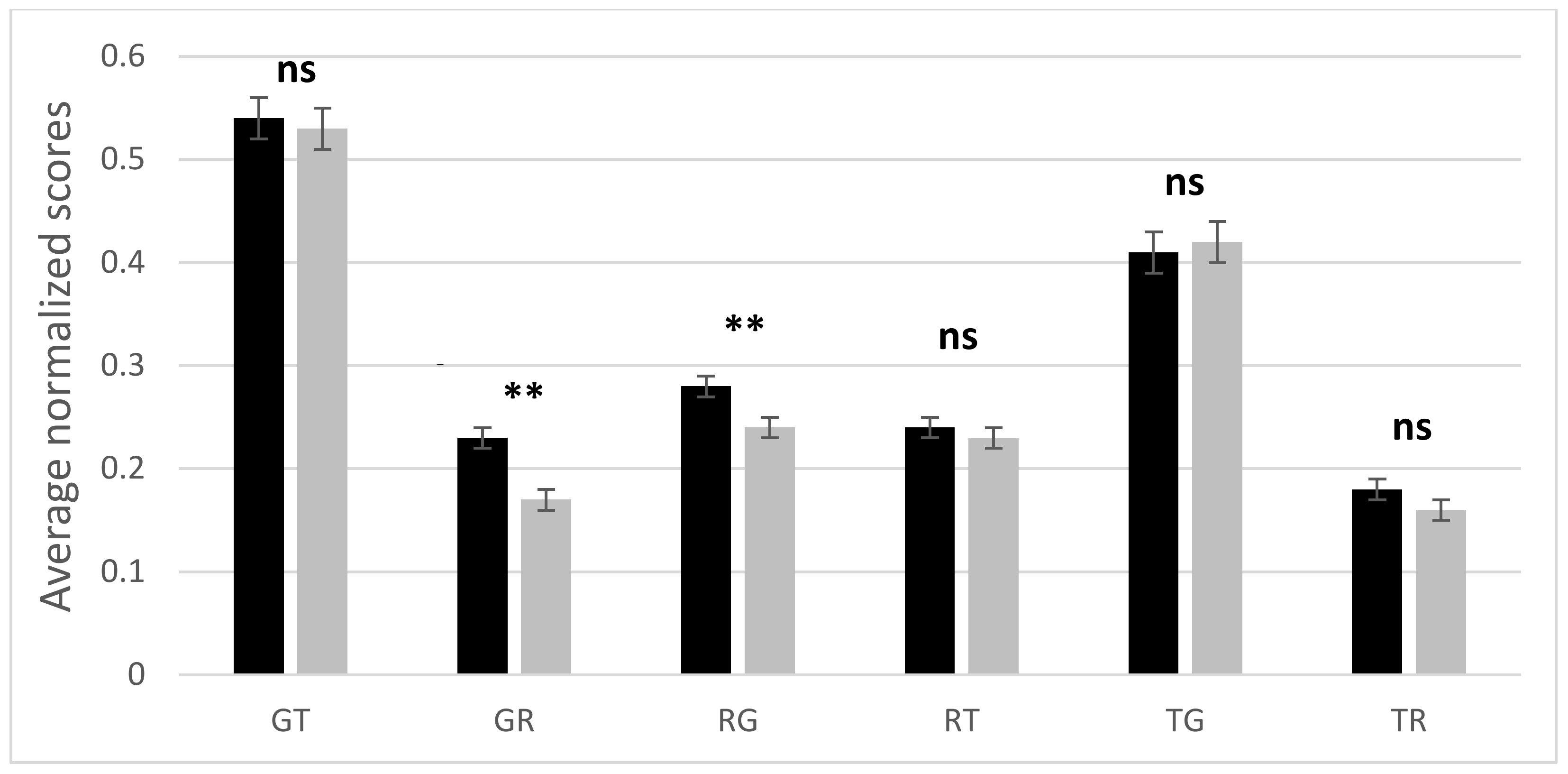
The average scores for the tests of kinematics and mathematics are (6.2 ± 0.2)/20 and (5.7 ± 0.2)/20, respectively. For most questions the frequency of correct answers is less than 50%, thus confirming that the sample involved in the study presents considerable difficulties in interpreting the graphical, tabular, and algebraic representations. In Figure 1 the normalized average scores, for all groups of transitions in kinematics and mathematics, are reported.
A paired samples t-test was carried out to compare the results for each transition in kinematics and mathematics. It is observed that the differences between the two contexts are significant only for transitions between graphs and formulas (in both verses). The participants reported better results with transitions that exclude formulas, while for the other transitions the average scores are higher when the formula is the starting representation. The analysis considering the types of function is shown in Figure 2.
The differences between the scores in kinematics and in mathematics are significant, except for decreasing functions with negative values. In general, the functions of type PP (i.e., increasing with positive values) are the simplest to deal with. There is a highly significant difference in the understanding of transitions for increasing and decreasing functions, both in kinematics (average score for increasing function = 0.32 ± 0.01; average score for decreasing function = 0.29 ± 0.01; t (642) = 4.633, p < 10−3, d = 0.18) and in mathematics (average score for increasing function = 0.30 ± 0.01; average score for decreasing function = 0.27 ± 0.01; t (642) = 5767, p < 10−3, d = 0.14). The average score for the NN group of functions (i.e., decreasing with negative values) in mathematics is the only one higher than the corresponding one in physics, but the differences are not significant. This aspect shows that, in the mathematical context, the parameters of the linear functions are confused with each other more easily than in physics, especially in the case of PN and NP groups of functions. In fact, the question with the lowest percentage of correct answers (9.3%) occurs in mathematics with the TR transition for an increasing function with negative values.
These results suggest the existence of common latent factors in the interpretation of the transitions presented in the tests. Four factors were obtained from the exploratory factor analysis:
  • Factor 1 = Transitions between graphs and tables, which gathers 12 questions, six from kinematics and six from mathematics, that require a transition between a graph and a table, in both directions. The average score for these items is 0.48 ± 0.01, while the McDonald’s Omega of the scale is 0.92.
  • Factor 2 = Transitions with formulas in physics, which groups together 14 kinematics questions that present an algebraic relationship as a starting or final representation. The average score is 0.24 ± 0.01, while the McDonald’s omega of the scale is 0.91.
  • Factor 3 = Transitions from formulas in mathematics, which gathers eight mathematics questions that have an algebraic relationship as starting representation. The average score is 0.23 ± 0.01, while the McDonald’s omega of the scale is 0.87.
  • Factor 4 = Transitions toward formulas in mathematics, which gathers six mathematics questions that have an algebraic relationship as the final representation. The average score is 0.17 ± 0.01, while the McDonald’s Omega on the scale is 0.52. This value suggests that the last scale is not reliable.
Therefore, we proceeded to re-analyze the eigenvalues of the factor analysis, and we tried to choose only the first three factors, thus combining factor 3 and factor 4: the new factor gathers 14 items that share an algebraic relationship as starting or final representation. The average score is 0.20 ± 0.01, while the McDonald’s Omega is 0.86.
These latent dimensions suggest that solving problems with graphs and tables requires the same cognitive ability, regardless of the physical or mathematical context, while the presence of relationships brings out different reasoning as the context varies (mathematics or kinematics). Furthermore, the type of function does not influence the factorization, therefore the type of transition is the characterizing feature of each question. The average score on the first latent factor differs significantly from each of the other two factors (t (642) > 3.9, p < 10−3, d > 0.20).

4.2. Confidence Scale

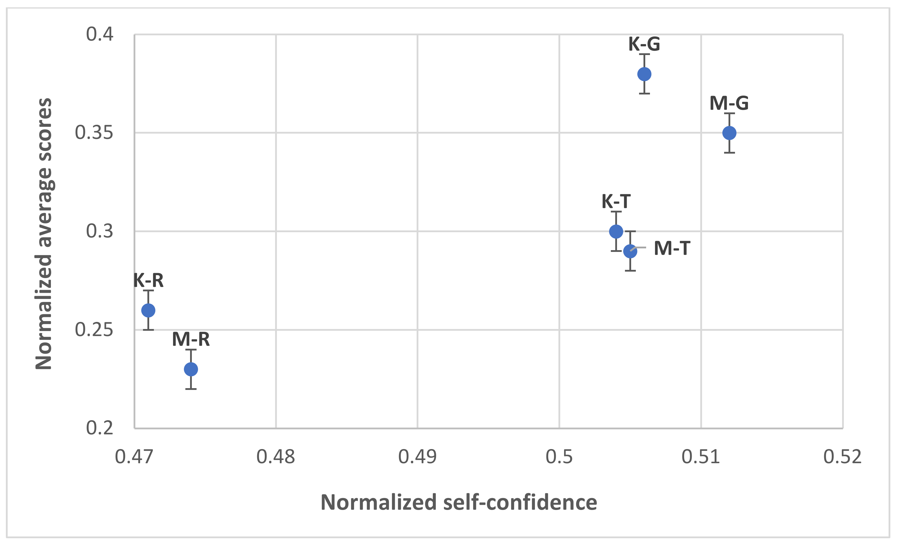
We report in Figure 3 the normalized average scores for the groups of knowledge questions characterized by the same starting representation, both in kinematics and mathematics, as a function of the corresponding self-confidence (normalized) score. We note that students feel more confident when the starting representation is a graph and less confident when the starting representation is a relationship, especially in kinematics.
The participants are substantially calibrated both in kinematics (average overconfidence = 0.18 ± 0.01) and in mathematics (average overconfidence = 0.19 ± 0.01). Figure 4 reports the normalized average scores for the accuracy of self-evaluation; paired samples t-tests show that the differences between mathematics and kinematics are significant, except for the transitions with tables as starting representations. The accuracy of self-evaluation scores is higher in mathematics, probably because of the higher amount of study dedicated to it, compared to physics. Moderately over-confident students are on average (namely considering the average percentage for the six groups of transitions identified) about 30% of the total, while the percentage of significantly over-confident students is about 18%. There are no significant differences in the accuracy of self-evaluation due to gender.

4.3. Questionnaires about the Orientation toward Physics

From the exploratory factor analysis carried out on the orientation toward physics items, two latent factors emerged (see Appendix B for the loading matrix), which we can interpret as follows:
  • Factor 1 = Self-regulation and Metacognition (McDonald’s omega = 0.89).
  • Factor 2 = Self-efficacy (McDonald’s omega = 0.82).
The average scores for these two dimensions are shown in Figure 5.
The other dimensions measured by the questionnaire, namely engagement and anxiety management, are excluded from the solution as the factor loadings of the corresponding items are lower than the established threshold.
We observe that the students show greater organization skills than problem-solving abilities: the differences between the two factors are statistically significant (t (642) = 8.213, p < 10−3, d = 0.60). The self-evaluation about problem-solving is significantly different between males and females (males’ average score = 3.09 ± 0.03; females’ average score = 2.89 ± 0.05; t (641) = 3.444; p < 10−3, d = 0.70), while for the first factor the differences are less significant (males’ average score = 3.17 ± 0.03; females’ average score = 3.30 ± 0.04; t (641) = −2.504; p = 0.13, d = 0.58).

4.4. Mental Rotation Test

The average score for the mental rotation test is very low (6.2 ± 0.2 out of 20). Gender differences in favor of the male gender are confirmed (males’ average score = 6.7 ± 0.2; females’ average score = 5.1 ± 0.3; t (641) = 4.371; p <10−3).

4.5. Linear Regression

We report in Table 2 the standardized regression coefficients obtained from the linear regression analysis, together with the correlation coefficient and the variance explained. We chose gender, self-confidence (both in kinematics and mathematics), the two dimensions of the orientation toward physics, and spatial ability as independent variables (namely their average scores, as described above). The normalized average scores in kinematics and mathematics, as well as those related to the three factors extracted by these tests, were selected as dependent variables. Overall, we have five dependent variables, for which we carried out a different regression analysis. If an independent variable does not affect the dependent one, the regression coefficient is not significant (ns).
It is also observed that, as expected, the score in the Mental Rotation Test is strongly predictive for all the dependent variables considered. Similarly, perceived confidence in kinematics is predictive of the outcome in kinematics and in the transitions with formulas in physics. Conversely, perceived confidence in mathematics is predictive, especially for performance for mathematics items. Gender correlates negatively with performance in mathematics in a slightly significant way, but this does not happen in kinematics. On the other hand, the orientation toward physics has a different impact depending on its factors: the dimension linked to the organization skills and the elaboration of information does not influence the outcomes, while self-efficacy is a strong predictor, especially in mathematics and for transitions that do not include algebraic formulas.

5. Discussion

In this section, we discuss the results obtained, answer the research questions, and present some implications of the study.

5.1. How Does the Representational Fluency Differ between Mathematics and Physics?

From the analysis carried out on the kinematics and mathematics items, most of the difficulties emerge when dealing with representational fluency in mathematics. We observed that the differences between the two contexts (kinematics and mathematics) are significant especially when it is necessary to identify the correlation between graphs and formulas (in both directions). In particular, for graphs, the differences between mathematics and physics also emerge in the case of elementary functions, such as those increasing and with positive values. The literature has shown that it is often difficult to distinguish a graph of the law of motion from the corresponding trajectory, but we would expect that in the mathematical context, where the variables play a more abstract role, it will be easier to interpret a y(x) function on an x-y plane through a system of Cartesian axes. Despite this, our data do not support this hypothesis, confirming the idea that, for instance, a kinematic graph can help students to understand the information reported in a table. About algebraic relations, the existence of two different factors relating to transitions with formulas, one in physics and the other in mathematics, suggests that the reasoning schemes adopted by students are different in the two contexts when they have to solve problems with algebraic relations. Conversely, tables and graphs seem to play the same role in the process of extracting and comparing information.
This interpretation can indirectly justify why students show misconceptions in kinematics that are resistant to traditional teaching, which is mainly focused on a training approach characterized by numerical manipulation of the quantities. Our findings thus suggest that a conceptual understanding of the phenomenon under study is not necessarily associated with the mathematical understanding of related formulas. Our study also shows that transitions involving algebraic relationships in physics are easier to understand for students than the same type of transitions in mathematics, although students’ perception is the opposite: in particular, students feel more confident in transitions with formulas in mathematics, while they give less correct answers in this context. This also happens with graphs and tables. These results also show that a lack of calibration about self-confidence can lead to not using all the cognitive resources necessary to solve this kind of problems.

5.2. How Does the Representational Fluency Differ between the Different Types of Linear Functions?

From the analysis carried out, difficulties mostly concern the interpretation of negative increasing functions and positive decreasing functions. Such evidence suggests a difficulty in understanding the meaning of the slope sign. This evidence also confirms that in these cases students apply reasoning based on plane geometry to interpret trends over time: for example, in the case of an increasing function with negative values, the line can be interpreted as the path of a body that moves away from the origin, but which at the same time approaches the abscissa. Similarly, in the case of a decreasing function with positive values, the line can be interpreted as the path of a body that moves away from the origin, following the hypotenuse of a right-angled triangle formed by the axes and the line. In both cases, the confusion between the law of motion and the trajectory is confirmed.

5.3. What Is the Influence of Self-Confidence, Orientation toward Physics, Spatial Ability, and Gender on Representational Fluency in Mathematics and Physics?

Data analysis confirms the role of spatial ability in the correct interpretation of graphs in both kinematics and mathematics. This is coherent with the results obtained by the authors of [12], who found correlations very similar to ours (between 0.28 and 0.32) between spatial ability and problem-solving skills which involve the interpretation of graphs, such as those of force and acceleration. As for the other independent variables measured in this study, the predominant role of confidence as a predictor of students’ performance is confirmed. In particular, the confidence in kinematics questions significantly influences not only the total score, but also the latent factor which represents the ability to interpret the transitions between graphs and tables, and the transitions with formulas in kinematics. Self-confidence in mathematics has a significant impact on the total score, while on the latent factors the effect is lower. Paradoxically, although slightly better results have been obtained in physics, the students show higher confidence in mathematics than in kinematics. This evidence confirms the results of international comparative studies (such as [19]) for which the perception of confidence is an index of how well students evaluate their knowledge, helping them to plan their study and review it critically. In our case, the participants do not show a relevant overconfidence bias, that is, they do not significantly overestimate themselves. The substantial calibration is justified by the fact that students, both in kinematics and in mathematics, show that they generally feel less confident in their own answers—on a scale from 1 to 5, the average score is about 2.5—especially when the starting representation is a formula, despite being a type of representation widely used in school practice. This result confirms that these students need to improve not only the preparation but also their perception of this preparation, as the latter can negatively impact performance and motivation in answering standardized questions correctly.
In our model, gender does not influence students’ performances, as well as the self-regulation and metacognition dimension, while self-efficacy is confirmed as the strongest predictor among the other dimensions of the “orientation toward physics” construct, as was expected looking at the literature [20].
The results of these linear regressions have to be interpreted within some limitations. First of all, the variance explained by the models is always lower than 30%, which is not a good percentage. Spatial ability was measured by a standardized instrument, as well as the performances in kinematics and mathematics, from which we were able to grasp the particular role played by the algebraic relationships in both contexts. Probably, the tool regarding the orientation toward physics should be improved in terms of several constructs, as the dimension representing engagement in the learning process could play an important role in predicting the students’ outcomes. We could not perceive it because of the distribution of the factor loadings, from which the distinction between the metacognitive activities regarding the information’s elaboration and the self-regulation of the study activities does not emerge, representing another result we did not expect. Furthermore, some of these dimensions could play a role as a mediator of the relationship, but in order to measure these effects we should be sure to deal with reliable variables. This is the way to improve the significance of the results presented, which can represent an exploratory base from which to start, also involving participants coming from different school courses and in an international context.
Finally, we can observe that the physics field in the “orientation toward physics” does not play a specific role, as it can be replaced with a more general study field, given the items’ formulation.

6. Conclusions

The aim of this research was to highlight how different representations of linear phenomena, such as uniform rectilinear motion, stimulate students’ different reasoning and resolution strategies. The results of this study can be exploited in didactic interventions for the first years of high schools, in which different aspects of a phenomenon are modeled using elementary representations such as graphs, tables, and algebraic relationships also for domains other than the ones analyzed here (e.g., economy). Furthermore, our results suggest that students’ difficulties in physics could be addressed through better use of tables and graphs, which present fewer conceptual obstacles than that involving algebraic relationships. Considering these results, it is desirable that more effective and targeted training will make teachers aware of the potential and limits of the different types of representation.
Author Contributions

Conceptualization, I.T.; methodology, I.T. and D.C.; software, I.T.; validation, I.T. and D.C.; formal analysis, I.T. and D.C.; investigation, I.T.; data curation, I.T. and D.C.; writing—original draft preparation, I.T. and D.C.; writing—review and editing, I.T. and D.C.; visualization, I.T. and D.C.; supervision, I.T. and D.C.; project administration, I.T.; funding acquisition, I.T. All authors have read and agreed to the published version of the manuscript.

Funding

This research received no external funding.

Institutional Review Board Statement

Not applicable.

Informed Consent Statement

Informed consent was obtained from all subjects involved in the study.

Data Availability Statement

Not applicable.

Acknowledgments

We thank the teachers participating in the project, who kindly submitted the test in their classes.

Conflicts of Interest

The authors declare no conflict of interest. The funders had no role in the design of the study; in the collection, analyses, or interpretation of data; in the writing of the manuscript; or in the decision to publish the results.

Appendix A

Appendix A.1. Test on Kinematics with the Corresponding Self-Confidence

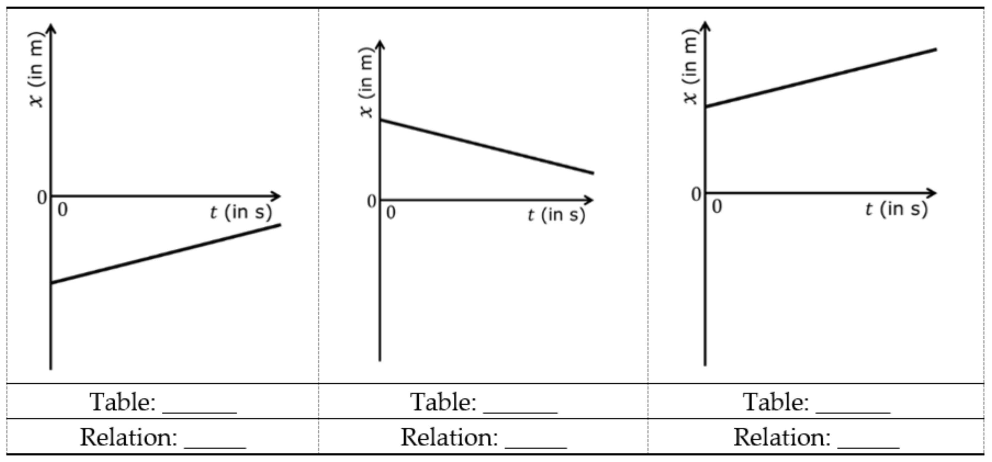
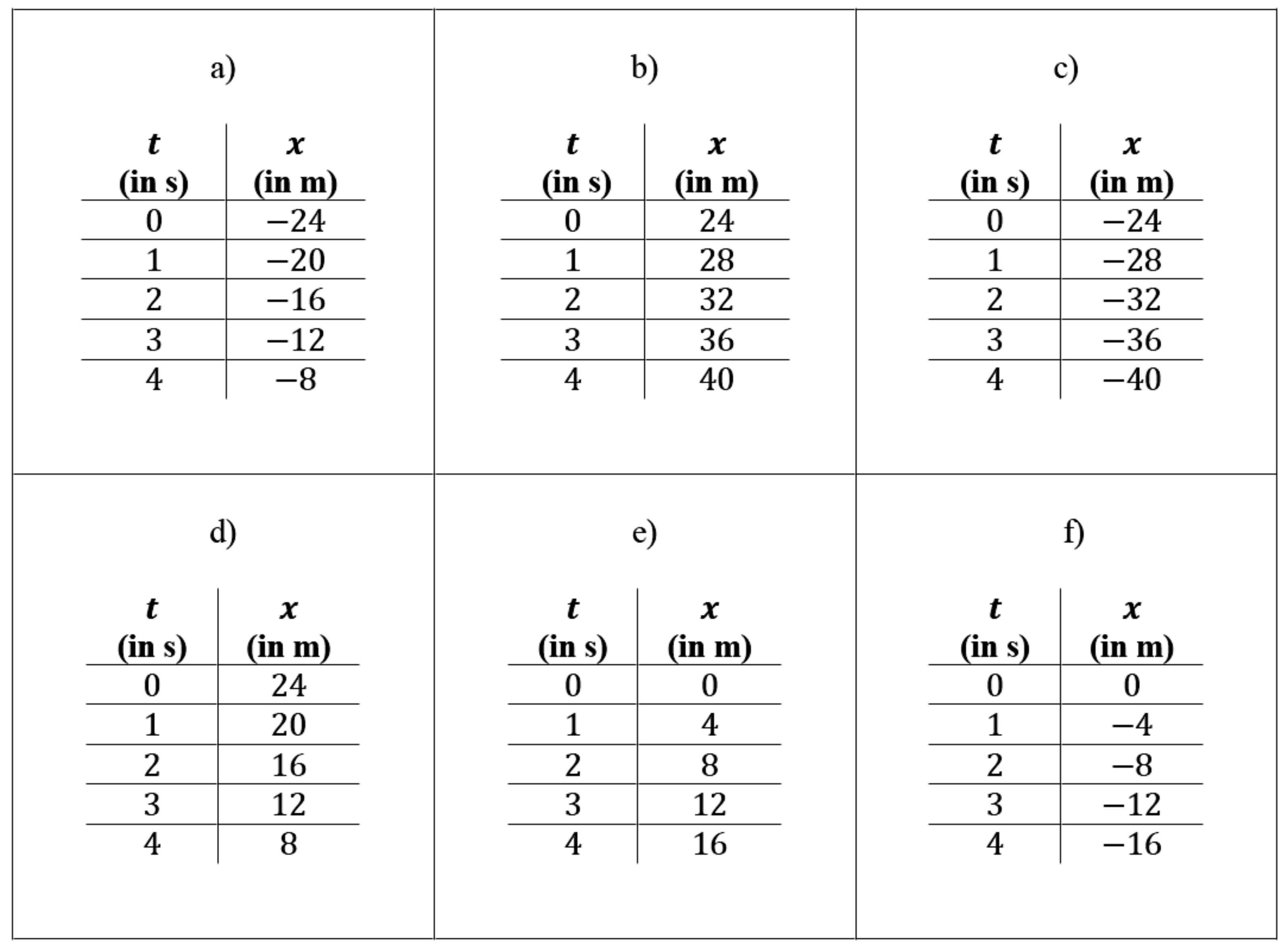
A cyclist is racing with a constant speed on a straight road. For each of the following 3 graphs (see Figure A1) which represent the position x in meters as a function of time t in seconds, indicate the table (see Figure A2) and the value of the parameters of the algebraic relationship x = x0 + vt (see Figure A3) that describes the cyclist’s motion.
Figure A1. Figure from the test on kinematics.
Education 12 00776 g0a1
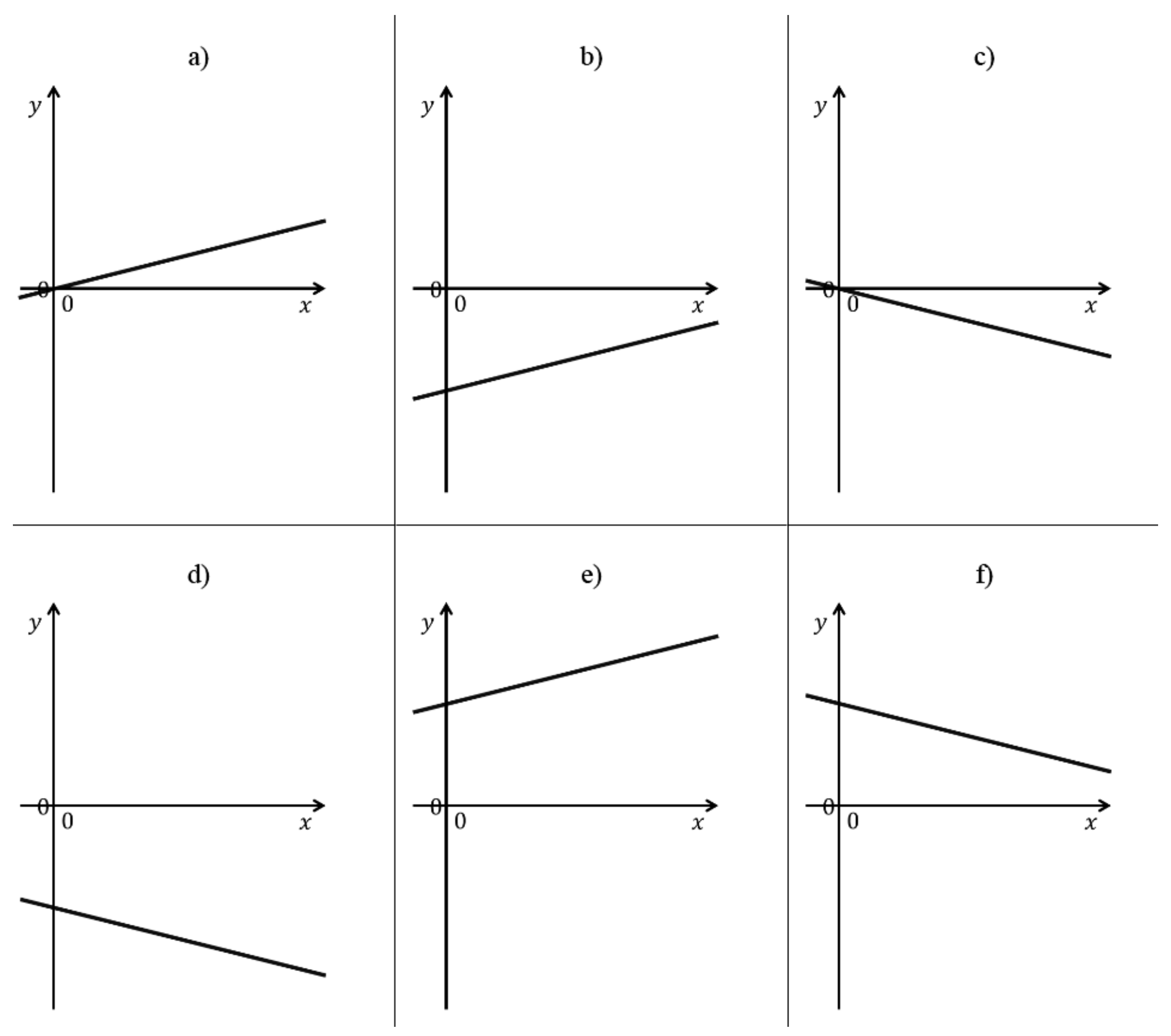
Figure A2. Figure from the test on kinematics. Subfigures (af) represent the possible options for the above question.
Education 12 00776 g0a2
Figure A3. Figure from the test on kinematics.
Education 12 00776 g0a3
How confident are you about your answers from 1 (not at all) to 5 (completely)?
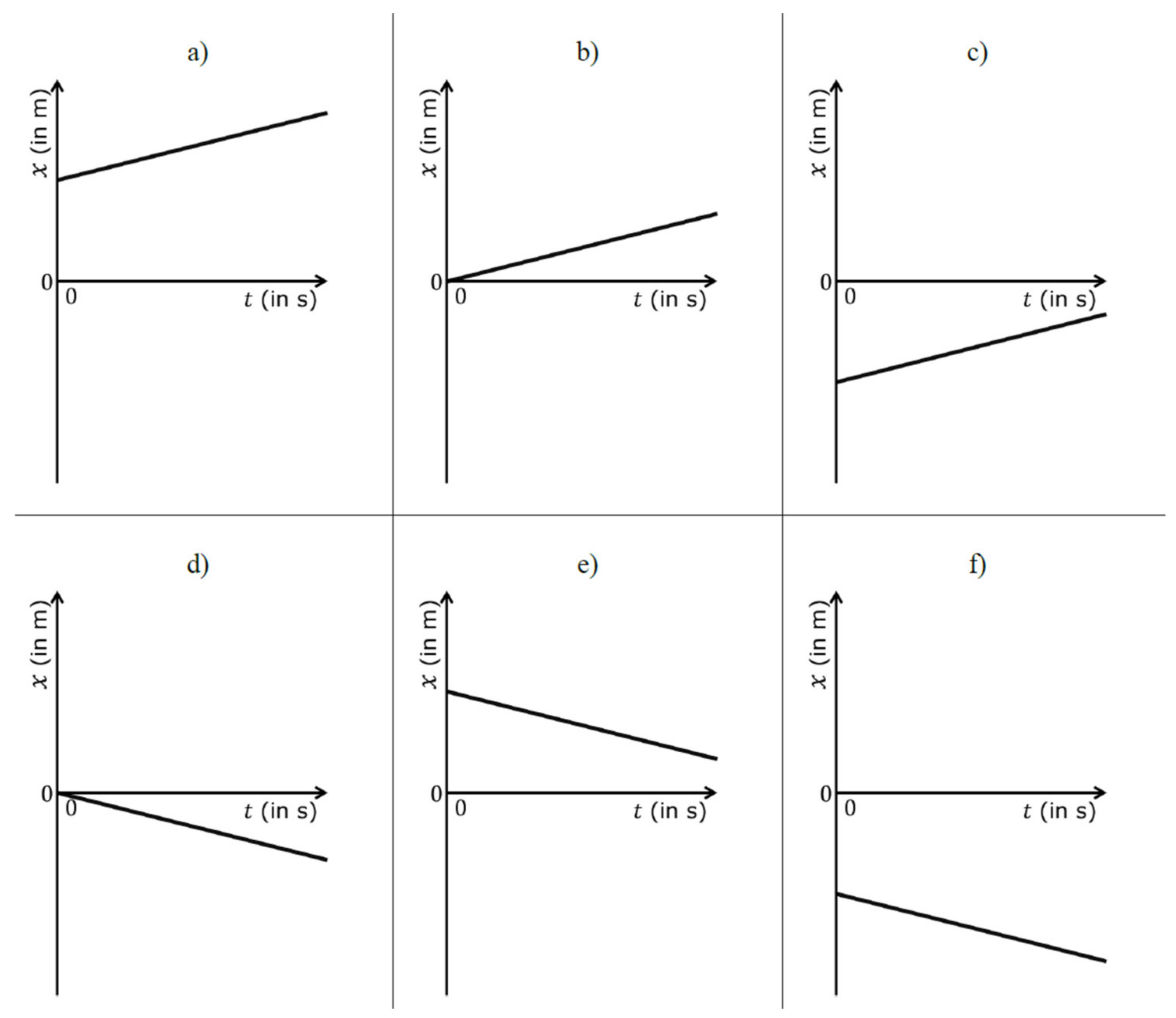
A car is moving on a road with a constant speed. The relationship between position x and time t is given by x = x0 + vt. Indicate which of the following graphs (see Figure A4) and which of the following tables (see Figure A5) represents the trend of position x as a function of time t when:
  • X0 > 0 and v > 0: Graph ______ Table ______
  • X0 > 0 and v < 0: Graph ______ Table ______
  • X0 < 0 and v > 0: Graph ______ Table ______
  • X0 < 0 and v < 0: Graph ______ Table ______
Figure A4. Figure from the test on kinematics. Subfigures (af) represent the possible options for the above question.
Education 12 00776 g0a4
Figure A5. Figure from the test on kinematics. Subfigures (af) represent the possible options for the above question.
Education 12 00776 g0a5
How confident are you about your answers from 1 (not at all) to 5 (completely)?
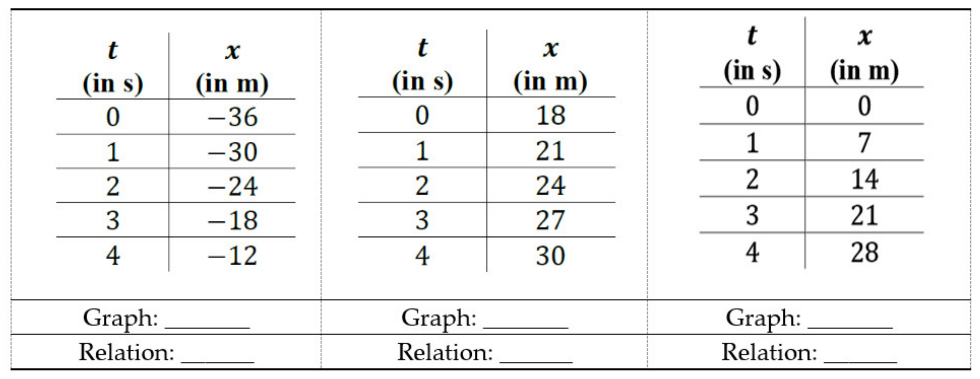
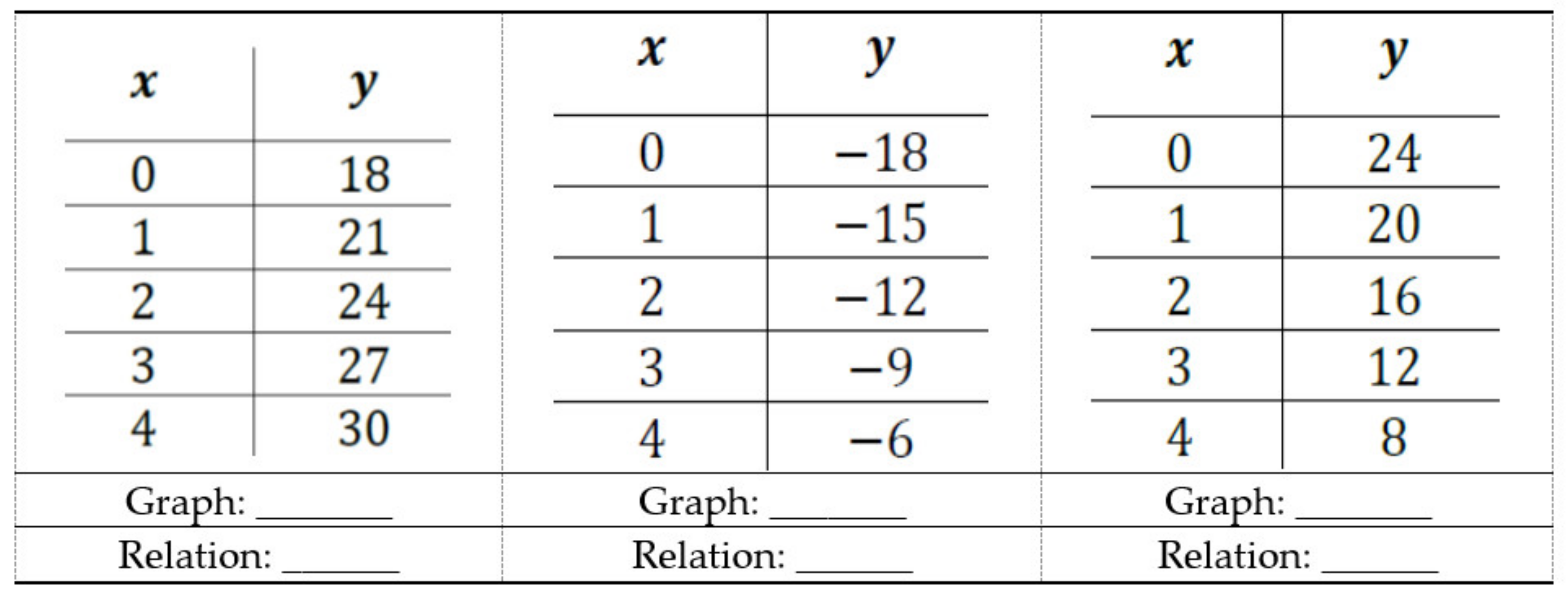
An airplane is traveling with a constant speed. For each of the three tables (see Figure A6) that describe the relationship between the position (in “m”) and the time (in “s”), indicate which graphs (see Figure A7) correspond to the table and the corresponding value of the parameters of the algebraic relationship x = x0 + vt (see Figure A8) which expresses the motion of the ‘airplane’:
Figure A6. Figure from the test on kinematics.
Education 12 00776 g0a6
Figure A7. Figure from the test on kinematics. Subfigures (af) represent the possible options for the above question.
Education 12 00776 g0a7
Figure A8. Figure from the test on kinematics.
Education 12 00776 g0a8
How confident are you about your answers from 1 (not at all) to 5 (completely)?

Appendix A.2. Test on Mathematics with the Corresponding Self-Confidence

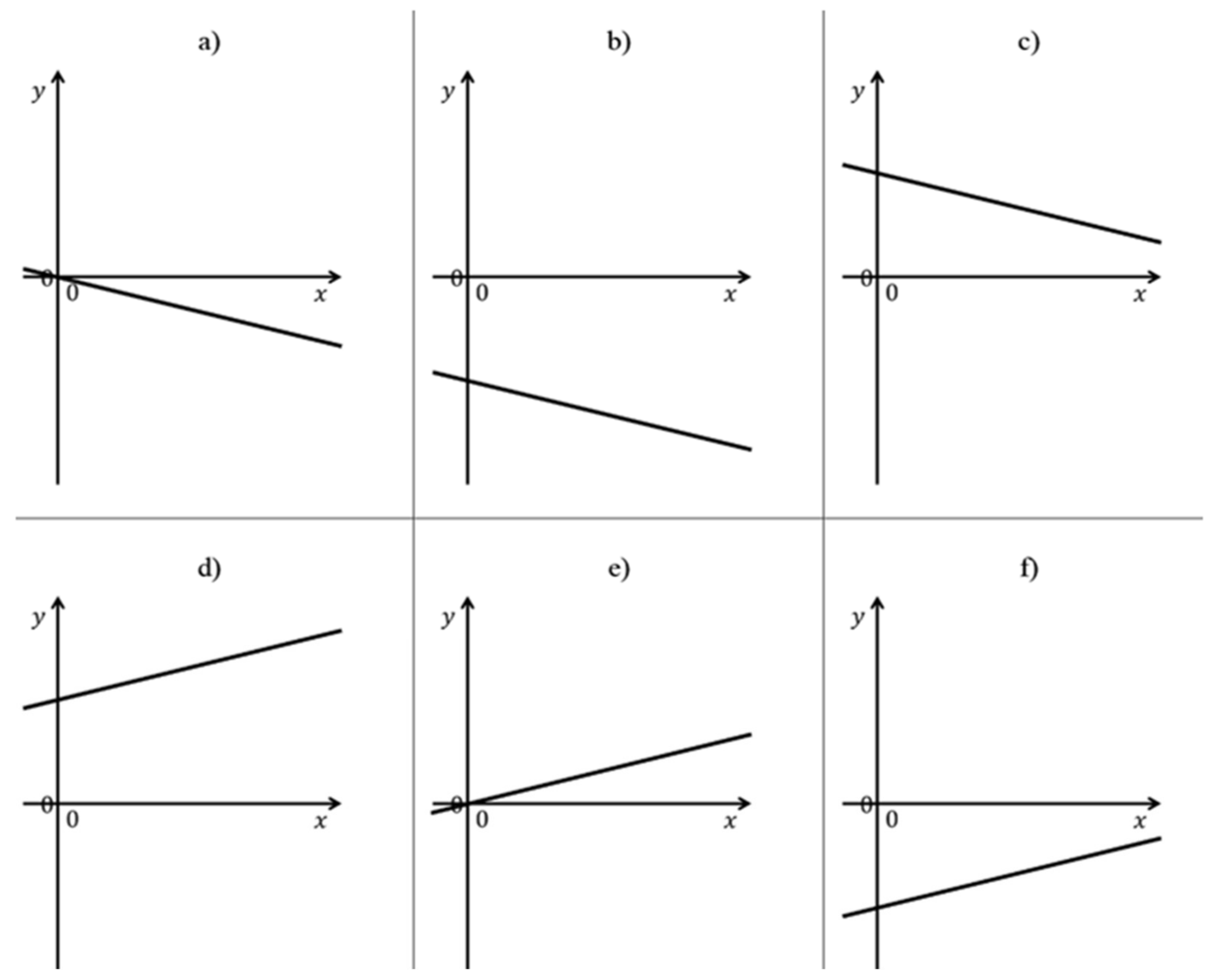
The variable y depends linearly on the variable x according to the formula y = ax + b. For each of the following 3 graphs (see Figure A9) that describe the relationship between y and x, indicate the corresponding table (see Figure A10) and the value of a and b (see Figure A11):
Figure A9. Figure from the test on mathematics.
Education 12 00776 g0a9
Figure A10. Figure from the test on mathematics. Subfigures (af) represent the possible options for the above question.
Education 12 00776 g0a10
Figure A11. Figure from the test on mathematics.
Education 12 00776 g0a11
How confident are you about your answers from 1 (not at all) to 5 (completely)?
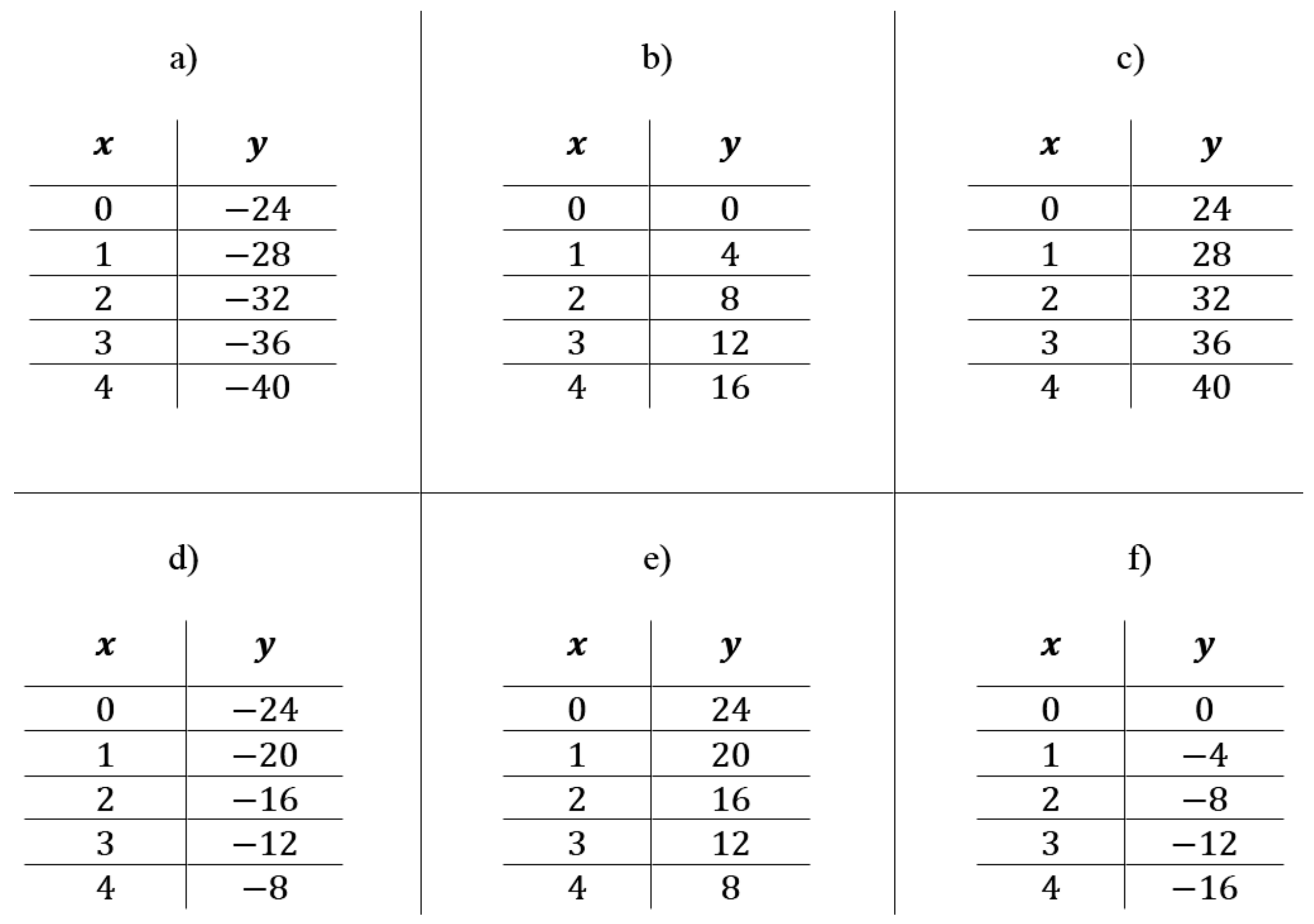
The variable y depends on the variable x according to the formula y = a + bx. Indicate which of the following graphs (see Figure A12) and which of the following tables (see Figure A13) represents the function when:
  • a > 0 and b > 0: Graph ______ Table ______
  • a > 0 and b < 0: Graph ______ Table ______
  • a < 0 and b > 0: Graph ______ Table ______
  • a < 0 and b < 0: Graph ______ Table ______
Figure A12. Figure from the test on mathematics. Subfigures (af) represent the possible options for the above question.
Education 12 00776 g0a12
Figure A13. Figure from the test on mathematics. Subfigures (af) represent the possible options for the above question.
Education 12 00776 g0a13
How confident are you about your answers from 1 (not at all) to 5 (completely)?
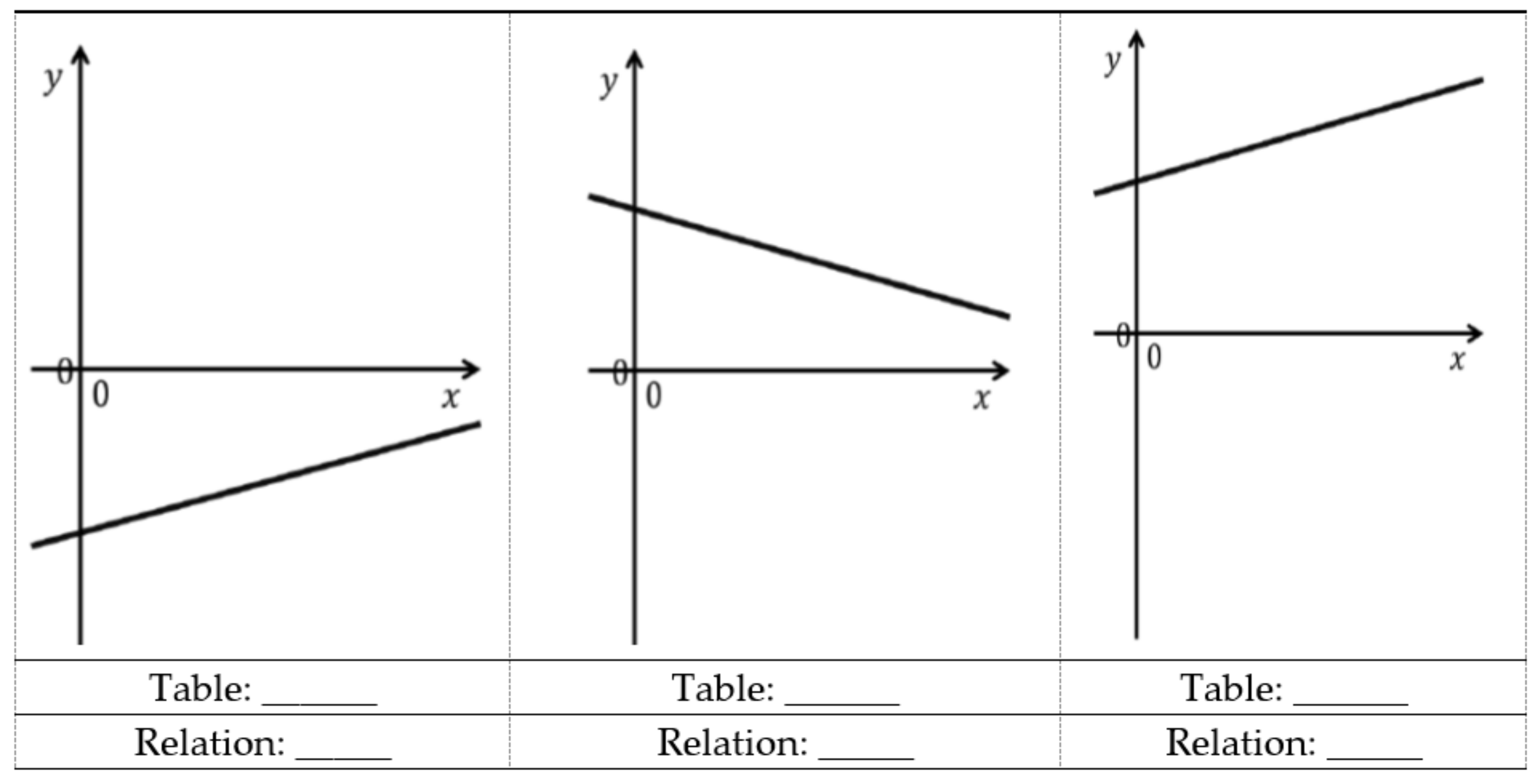
The variable y depends linearly on the variable x according to the formula y = ax + b. Indicate for each of the tables below (see Figure A14), the corresponding graph (see Figure A15) and the corresponding values of a and b (see Figure A16):
Figure A14. Figure from the test on mathematics.
Education 12 00776 g0a14
Figure A15. Figure from the test on mathematics. Subfigures (af) represent the possible options for the above question.
Education 12 00776 g0a15
Figure A16. Figure from the test on mathematics.
Education 12 00776 g0a16
How confident are you about your answers from 1 (not at all) to 5 (completely)?

Appendix B

Loading Matrix of the Orientation toward Physics Items

Here we report the loading matrix (see Table A1) obtained from the exploratory factor analysis of the questionnaire on orientation toward physics.
Extraction method: factorization of the main axis.
Rotation method: Promax with Kaiser normalization.
The saturation coefficients with an absolute value lower than 0.4 have been suppressed.
Some items do not saturate on any factor.
Table A1. Loading matrix obtained from the exploratory factor analysis on the orientation toward physics items.
ItemsAbility in Organizing Study, Information Processing and Class ParticipationAbility to Solve Problems and Manage Emotions
Maintain a constant rate of study throughout the school year0.757
Use the available study materials effectively (textbook, notes, etc.)0.696
Organize home study time effectively0.673
Take clear notes when the teacher explains0.660
Keep your concentration high during the lesson, even when your classmates are disturbing0.657
Always respect the established study program 0.629
Grasp and rework the essential contents of a lesson 0.622
Adapt my study method to the topics I am studying0.585
Plan the study according to the difficulty of the topics0.576
Rework the topics studied in written form adequately0.557
Establish achievable performance goals by evaluating my abilities and limits0.547
Attend lessons consistently0.527
Be constant in studying to get good marks at the end of the school year 0.519
Understanding the most important concepts0.497
Making connections and identifying similarities and differences in the different materials I am studying 0.433
Solving problems alone
Knowing how to find links with other subjects
Present in oral form the topics I have studied
adequately
Intervene in class to ask the teacher for further
explanation
Write my reasoning in the problems
Participate in class discussion actively
Managing anxiety before a task or an exam
Don’t be discouraged by a bad mark
Focus on the main concepts
Solving problems alone 0.806
Solve simple problems and exercises correctly 0.725
Knowing how to apply simple formulas 0.676
Set up problems by yourself 0.561
Knowing how to read graphs and tables 0.554
Solve complicated problems correctly 0.554

References

  1. Available online: https://www.oecd.org/pisa/publications/pisa-2018-results-volume-i-5f07c754-en.htm (accessed on 1 February 2021).
  2. Testa, I. Il ruolo della fisica nell’alfabetizzazione scientifica e nei processi di decisione degli studenti riguardo questioni socio-scientifiche: Analisi di una sperimentazione didattica. Giornale di Fisica 2012, 53, 199–234. [Google Scholar]
  3. Trowbridge, D.E.; McDermott, L.C. Investigation of student understanding of the concept of velocity in one dimension. Am. J. Phys. 1980, 48, 1020. [Google Scholar] [CrossRef]
  4. Trowbridge, D.E.; McDermott, L.C. Investigation of student understanding of the concept of acceleration in one dimension. Am. J. Phys. 1981, 49, 242. [Google Scholar] [CrossRef]
  5. McDermott, L.C.; Rosenquist, M.L.; van Zee, E.H. Student difficulties in connecting graphs and physics: Examples from kinematics. Am. J. Phys. 1987, 55, 503. [Google Scholar] [CrossRef]
  6. Beichner, R.J. Testing student interpretation of kinematics graphs. Am. J. Phys. 1994, 62, 750. [Google Scholar] [CrossRef]
  7. Giberti, G.; Monroy, G.; Sassi, E. Difficoltà di apprendimento in cinematica di studenti del I anno del corso di laurea in matematica. La Fisica nella Scuola 1997, 30, 10. [Google Scholar]
  8. Planinic, M.; Milin-Sipus, Z.; Katic, H.; Susac, A.; Ivanjek, L. Comparison of student understanding of line graph slope in physics and mathematics. Int. J. Sci. Math. Educ. 2012, 10, 1393–1414. [Google Scholar] [CrossRef]
  9. Kozhevnikov, M.; Motes, M.A.; Hegarty, M. Spatial visualization in physics problem solving. Cogn. Sci. 2007, 31, 549–579. [Google Scholar] [CrossRef] [PubMed]
  10. Pospiech, G.; Geyer, M.A.; Ceuppens, S.; De Cock, M.; Deprez, J.; Dehaene, W.; Michelini, M.; Stefanel, A. Role of graphs in the mathematization process in physics education. J. Phys. Conf. Ser. 2019, 1287, 012014. [Google Scholar] [CrossRef]
  11. Susac, A.; Bubic, A.; Kazotti, E.; Planinic, M.; Palmovic, M. Student understanding of graph slope and area under a graph: A comparison of physics and nonphysics students. Phys. Rev. Phys. Educ. Res. 2018, 14, 020109. [Google Scholar] [CrossRef] [Green Version]
  12. Kozhevnikov, M.; Thornton, R. Real-time data display, spatial visualization ability, and learning force and motion concepts. J. Sci. Educ. Technol. 2006, 15, 111–132. [Google Scholar] [CrossRef]
  13. Ceuppens, S.; Deprez, J.; Dehaene, W.; De Cock, M. Design and validation of a test for representational fluency of 9th grade students in physics and mathematics: The case of linear functions. Phys. Rev. Phys. Educ. Res. 2018, 14, 020105. [Google Scholar] [CrossRef]
  14. Lindsey, B.A.; Nagel, M.L. Do students know what they know? Exploring the accuracy of students’ self-assessments. Phys. Rev. Phys. Educ. Res. 2015, 11, 020103. [Google Scholar] [CrossRef] [Green Version]
  15. Bandura, A. Autoefficacia: Teoria e Applicazioni; Erickson Editore: Trento, Italy, 2000. [Google Scholar]
  16. Marzoli, I.; Colantonio, A.; Fazio, C.; Giliberti, M.; Scotti di Uccio, U.; Testa, I. Effects of emergency remote instruction during the COVID-19 pandemic on university physics students in Italy. Phys. Rev. Phys. Educ. Res. 2021, 17, 020130. [Google Scholar] [CrossRef]
  17. Hegarty, M. Spatial thinking in undergraduate science education. Spat. Cogn. Comput. 2014, 14, 142–167. [Google Scholar] [CrossRef]
  18. Vandenberg, S.G.; Kuse, A.R. Mental rotations, a group test of three-dimensional spatial visualization. Percept. Mot. Ski. 1978, 47, 599. [Google Scholar] [CrossRef]
  19. Morony, S.; Kleitman, S.; Lee, Y.P.; Stankos, L. Measures of the trait of confidence. Int. J. Educ. Res. 2015, 158–189. [Google Scholar] [CrossRef]
  20. Lin, T. Multi-dimensional explorations into the relationships between high school students’ science learning self-efficacy and engagement. Int. J. Sci. Educ. 2021, 43, 1193–1207. [Google Scholar] [CrossRef]
Figure 1. Normalized average scores in kinematics (black) and mathematics (gray) for type of transition between different representations (see methods section for definitions). Whiskeys for each vertical bar represent the standard errors of the average score. The significance (p) of the t-tests, carried out to compare the two contexts for each type of transition, was classified into two ranges: p > 0.05 → ns (not significant differences); p < 0.01 → ** (highly significant differences).
Education 12 00776 g001
Figure 2. Normalized average scores in kinematics (black) and mathematics (grey) for type of function represented (see definition in the methods section). Whiskeys for each vertical bar represent the standard errors of the average score. The significance (p) of the t-tests, carried out to compare the two contexts for each type of function, was classified into three ranges: p > 0.05 → ns (not significant differences); 0.01 ≤ p ≤ 0.05 → * (significant differences); p < 0.01 → ** (highly significant differences).
Education 12 00776 g002
Figure 3. Trend of the normalized average scores for the kinematics (K) and mathematics (M) knowledge questions with tables (T), graphs (G), and algebraic relations (R) as starting representations, as function of the corresponding self-confidence.
Education 12 00776 g003
Figure 4. Normalized average scores of the accuracy of self-evaluation in kinematics (black) and mathematics (grey). The whiskey for each bar represents the standard errors of the average score. The significance (p) of the t-tests, carried out to compare the two contexts for each type of transition, was classified into three ranges: p > 0.05 → ns (not significant differences); 0.01 ≤ p ≤ 0.05 → * (significant differences); p < 0.01 → ** (highly significant differences).
Education 12 00776 g004
Figure 5. Average scores for the dimensions of the orientation toward physics measurement. The vertical bars for each column represent the standard errors of the scores.
Education 12 00776 g005
Table 1. McDonald’s Omega values and sample size for each instrument.
SurveysMcDonald’s OmegaNumber of ItemsNumber of Participants
Kinematics0.9220643
Mathematics0.8920643
MRT0.8820643
Self-confidence (kinematics)0.893643
Self-confidence (mathematics)0.873643
Orientation toward physics0.9230643
Table 2. Standardized regression coefficients. Legend: * 10−3p ≤ 0.05; ** p < 10−3; “ns” means “not significative influence” (p > 0.05).
Variables: Dependent →
Independent
KinematicsMathematicsTransitions between Graphs and Tables Transitions with Formulas in KinematicsTransitions with
Formulas in Mathematics
Correlation coefficient0.530.520.470.500.47
Variance explained (%)2827222421
Gender−0.03 ns−0.07 *−0.00 ns−0.05 ns−0.09 *
Self-
confidence (kinematics)
0.29 **0.12 *0.15 *0.28 **0.15 *
Self-
confidence (mathematics)
0.09 ns0.22 **0.14 *0.09 ns0.19 *
Self-regulation and Metacognition 0.16 ns0.02 ns−0.03 ns0.05 ns0.05 ns
Self-efficacy0.11 *0.16 **0.15 **0.11 *0.11 *
Spatial ability0.26 **0.21 **0.24 **0.22 **0.18 **
Publisher’s Note: MDPI stays neutral with regard to jurisdictional claims in published maps and institutional affiliations.