1. Introduction
Most people with average spatial abilities can draw a cuboid, and, vice versa, can observe a cuboid from a line drawing. Of course, depending on the personal drawing abilities and cultural background, this drawing as well as the perception and understanding of this drawing can be diverse (see, e.g., [
1]). Having that said, in spatial line drawings of artistic pieces, design materials and mathematics illustrations, we can distinguish fundamentally two basic approaches: the axonometric (or oblique) type, when the parallel sides of the cube will also be parallel in the drawing, and the perspective type, when—due to the classical rules of perspectivity—images of lines of parallel edges meet at one point (the so-called vanishing point) in some or all of the three directions.
It is by no means trivial whether a drawing is well understood by the observer and if this is a correct drawing to provide the specific mathematic knowledge or artistic message [
2,
3,
4]. This holds already in the case of a simple cube [
5,
6]. Accurate drawing and understanding of a drawing is of utmost importance to effectively support mathematical performance [
7], especially in geometry [
8], but its interdisciplinary impact is also crucial. Understanding and representing spatial relationships are fundamental skills in many fields, and the development of these skills can have a mutual impact on various disciplines from pure mathematics to arts [
9].
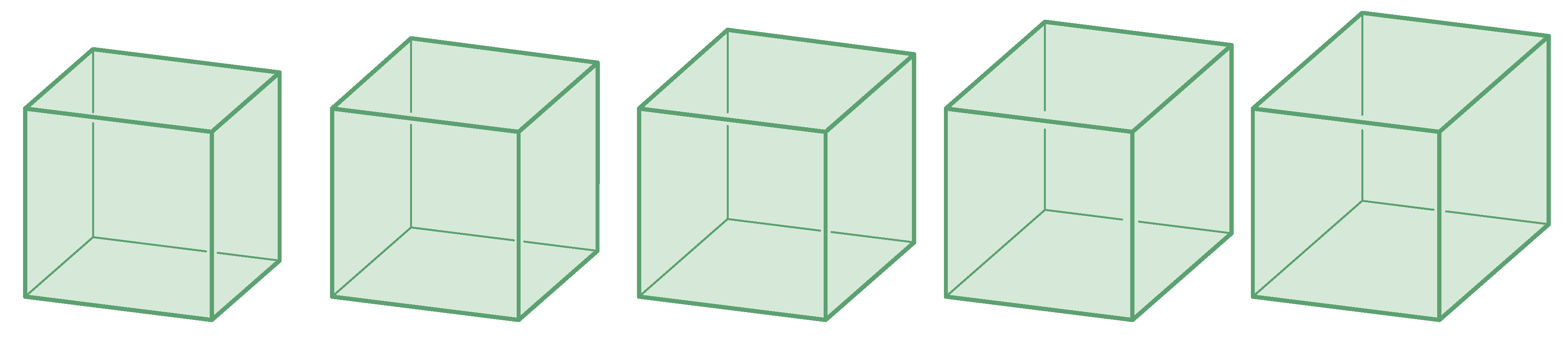
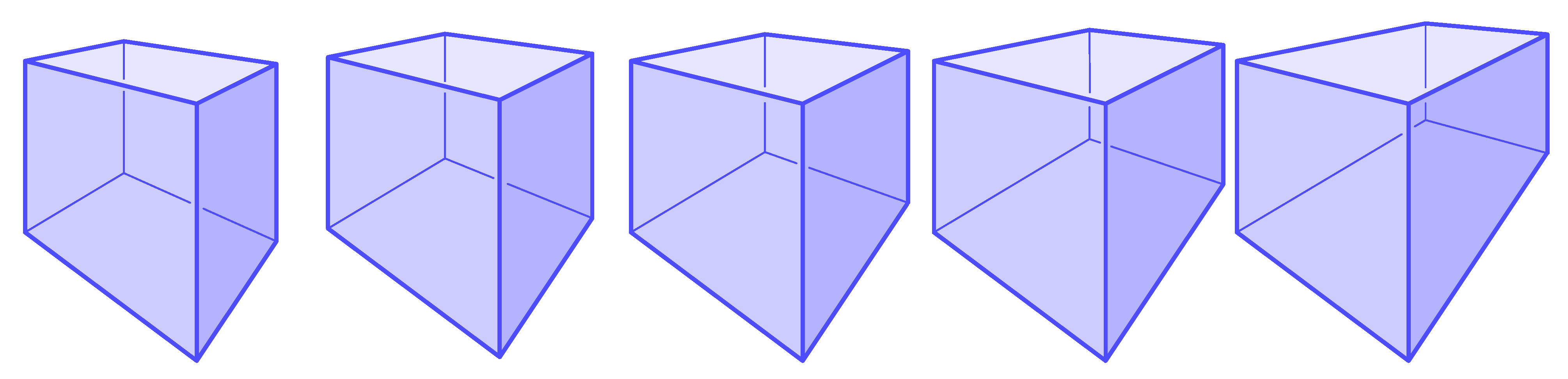
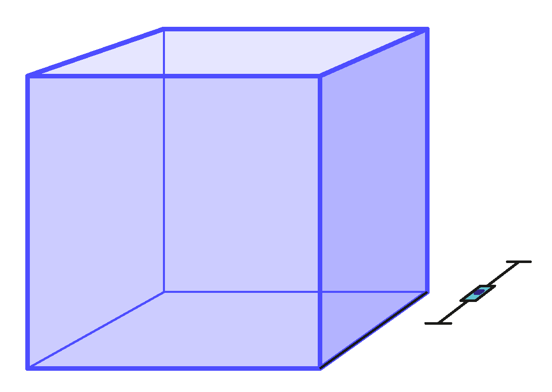
Our central question in this study is whether a correct line drawing depicts a general cuboid (i.e., a box-like polyhedron with six rectangular sides but different edge lengths in the three dimensions) or indeed a cube, that is, a cuboid with three spatial dimensions of the same length. The proportions of the three edge-lengths of the image of a cuboid, including the foreshortening or depth ratio, can be chosen in the drawing in many different ways (see
Figure 1 and
Figure 2); therefore, there is no unique correct way of drawing a cube.
However, does (and if yes, when) a specific drawing really depict a cube and not a general cuboid? And can we observe this difference? In this paper, we look for an answer to whether there is a common visual sense in this observation, whether there is a specific ratio of width, height and depth of the figure along the three dimensions when people generally feel that they are really watching a cube.
To do this, we conducted an experiment with an interactive computer model in which the width and height of the cuboid drawing are fixed, but the foreshortening in the third direction (the “depth”) can be changed by the user with simple means [
10]. This is an innovative investigation because although students are taught to see and draw the representation of the cube, no previous investigation has been carried out on the visual perception of these drawings. We were interested in how coherent people, who were actually first-year students with advanced spatial perception skills (c.f. [
11]), but without specific knowledge of descriptive geometry principles, judge this situation, and to what extent the set foreshortenings coincide or differ for different students. In the case of axonometric drawing, we have also compared the selected depth of the cube to the foreshortening conventionally used in engineering drawings and figures in educational materials. In the case of perspective drawings, we have examined how these positions are coherent to the exact solution of this problem in the geometric sense (what we mean by the exact solution here will be discussed in detail in
Section 2).
It is essential to understand what people will perceive from a geometric spatial drawing on a blackboard or a canvas, which is related to the question of perceiving extents and distance (for an overview of this question, see [
12]).
The main outcome of this study is that there is a somewhat common sense of observing a cube (and not a cuboid), but there is a small number of people who have a significantly different view of these drawings. Moreover, while this common sense highly coincides with the conventional and geometrically correct drawing and selection of foreshortenings, in some particular cases, there is a significant discrepancy between perception and convention. This all must be taken into account when a figure, an illustration or an artistic drawing is used to explain spatial relationships.
In the following section, we briefly review the geometric background of the two types of representation. In
Section 3, we describe the data collection and analysis. In
Section 4, results of the experiment are presented in detail. Conclusions close the paper in
Section 5.
2. Geometric Background
Consider first the so-called axonometric representation, which plays a crucial role in many applications in knowledge production (for a detailed discussion of this method, see, e.g., [
13]). An axonometric image of a cube or any general cuboid is fairly easy to produce. For simplicity, imagine that the three extensions of the cuboid are in the
x,
y, and
z axes mutually perpendicular to each other, with one vertex at the origin. Let us fix a point, the image of the origin, in the drawing plane and three half-lines starting from it, the images of the three axes. Taking an additional vertex on each of these half-lines, separately, the image of the cuboid is already uniquely defined, we only need to draw parallel segments from the corresponding points to finalize the figure. If the spatial cube is considered to be of unit edge-length, then it is evident that in the drawing, not all edges of the image will necessarily be of unit length, but the parallel edges will be the same length in each direction. The ratio of the original edge length to the edge length shown in the drawing is characterized by the foreshortening values
,
, and
in the three directions, separately. These values can freely be chosen by the person who prepares the drawing.
The axonometric representation is closely related to parallel projection. While in the former, as we have seen above, one can draw the image with a great deal of freedom after observing the spatial shape (cuboid), and in parallel projection, the image of the spatial cuboid is prepared through a projection onto the plane with rays parallel to a predefined direction. One of the central questions in axonometry is that if we draw a cuboid with arbitrary axial directions and arbitrary foreshortenings
,
, and
in the above way, then there exists a spatial cube in some position whose image through a parallel projection with a well-chosen direction will exactly coincide with the original drawing. Pohlke’s famous theorem gives a positive answer to the question: no matter how we draw the axonometric image of the cuboid, it can be not only the image of a general cuboid but also a parallel projection of a cube, well-positioned in space [
14].
Thus, according to Pohlke’s theorem, any axonometric image of a cuboid can be considered a cube. However, it is clear that in the case of a very elongated image, most observers associate it with a general cuboid rather than a cube. In our experiment, we examined whether there was any “common sense” about the axonometric image of a cuboid being a cube.
Persons were given an axonometric drawing depicting a cuboid where the foreshortening was fixed in two directions (the edge lengths of width and height were predefined in the image), but in the third direction, persons were able to freely adjust the edge length in an interactive way. Our request was to adjust this third-direction foreshortening until they themselves observe the image as a cube, and not as a cuboid with different side lengths. Here, we emphasize once again that in the case of an axonometric mapping, there is no single solution, no specific “perfect” drawing according to Pohlke’s theorem. That is, in principle, any foreshortening is equally good from a geometric point of view, in all cases the drawing can be considered as an image of a cube. However, as our results show, the foreshortenings set by testing persons, with a few exceptions, were clearly culminated around a single value. All this means is that for each setting, there is some kind of common sense as to whether this image represents a cube.
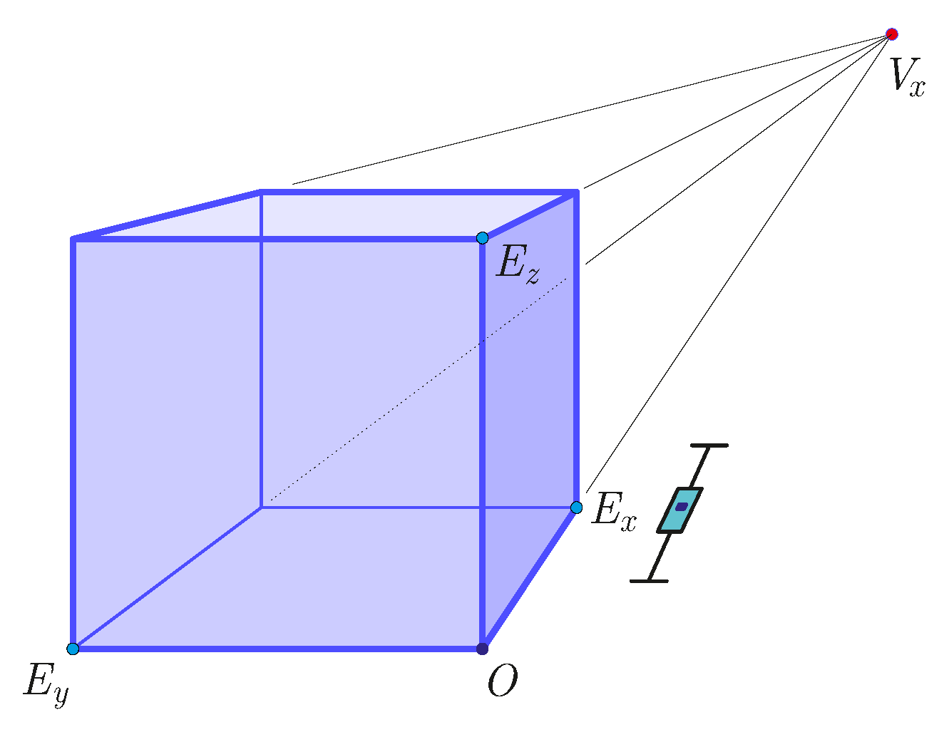
In the case of perspective images, the story is a bit different. The essence of the perspective representation is that the images of lines of parallel edges in space converge at a point (the so-called vanishing point) in the drawing. This method of graphical representation results in a much more realistic figure than the axonometric image and has deeply influenced art and science since the Renaissance.
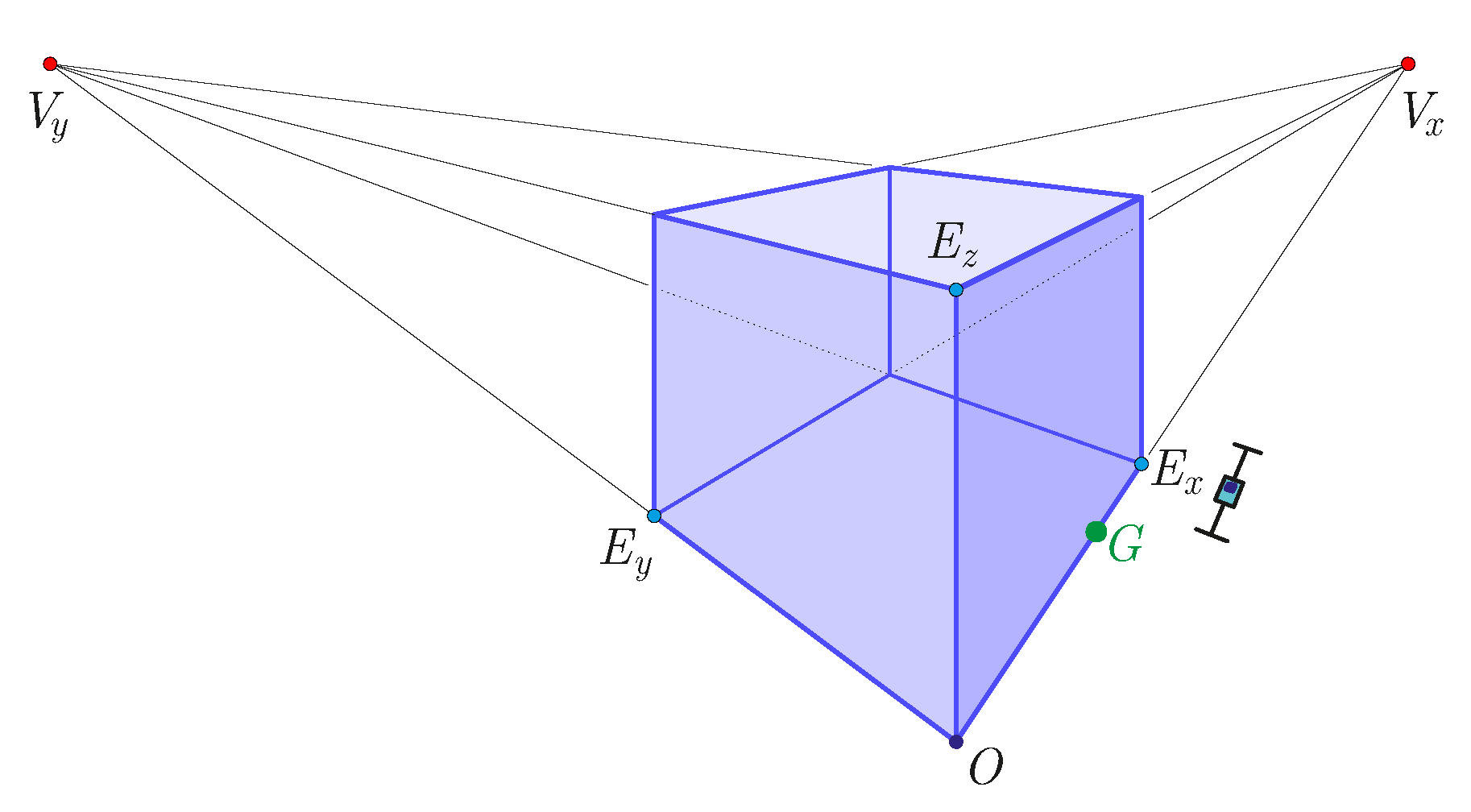
Imagine a cuboid again with three edges in the directions of x, y and z axes perpendicular to each other and one vertex in the origin. Let us define a point (the image of the origin) in the drawing and the three half-lines starting from it; hence, we have fixed the image in the three directions. Contrary to the axonometric drawing, however, on these half-lines we must define not only one additional vertex (the image of the unit point) but also, along the directions, we must determine the points at which the lines parallel to the given direction intersect each other. These latter points are called vanishing points. If we select such a point in each of the three directions, the image will be called a three-point perspective (see points in perspective figures, but if we define these points in only one or two directions, while lines in the other directions remain parallel, we obtain a one-point and two-point perspective drawing, separately. The perspective image of the cuboid thus becomes uniquely defined by selecting the origin, the axes (half lines), the unit points, and the vanishing points: if these are given, the image of the cuboid is uniquely determined and can be easily drawn.
The perspective representation is closely related to central projection. If a spatial cuboid is projected from a center to the image plane, then the result is a perspective image of the cuboid. A question similar to the axonometric case can be asked: if one prepares a perspective drawing of a cube specifying the origin, the three arbitrary directions, the unit points and vanishing points along these directions, is there a cube in space and an appropriate center of projection, from which we obtain the given image by projecting the cube from that center onto the plane? Whilst the answer was always positive in the axonometric case for any drawing, the answer is negative in almost every case of a perspective drawing. The one-point perspective can always be considered as an image of a centrally projected cube. However, given a two- or three-point perspective drawing, there are a number of conditions that must be met in order to find a spatial cube and a projection center from which the cube can be projected to obtain the given image. For an overview of these conditions, see, e.g., [
15,
16,
17].
In other words, for most perspective drawings, there is no appropriate spatial structure from which we can receive an analogous visual perception. If we fix the origin, the three directions, the (two or three) vanishing points and two out of three unit points, as it happened in our experiment, then the mathematical conditions mentioned above allow us to determine the only position of the third unit point, for which such a central projection exists. In all the other cases, the perspective drawing can be correct in itself, but cannot be the result of a central projection.
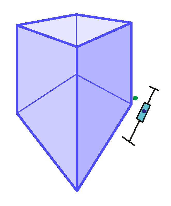
We have conducted the experiment related to perspective drawings similarly to the case of axonometric drawings. Persons were given a perspective image depicting a cuboid where the vanishing points were given in all three directions, the side length was also fixed in two directions, but in the third direction, persons were able to adjust the side length at will. Our request was to adjust this third direction length (“depth” of the cuboid) until they themselves feel they see the image of a cube and not a cuboid with different side lengths. As we have discussed above, unlike axonometry, not all positions here are correct in a geometric sense, i.e., there was practically one single position in each figure that actually resulted in an image that could be the central projection of a cube. This single correct position of the third unit point has been calculated and visualized as a green unit point in each of the perspective figures with two or three vanishing points.
In our experiment, the foreshortenings set by students in most of the cases showed a surprising coincidence in the case of perspective drawing as well. Moreover, with a good approximation, the adjusted vertex was positioned close to the only geometrically correct position. All this means, surprisingly, is that there is common sense in terms of the perception of perspective images as well as whether this image represents a cube.
3. Method of the Survey
For our investigation, we created a twenty-drawing-questions online test. Test figures were created by GeoGebra. Given a slider tool, students were able to find the best position of the adjustable side length of the cube in each of the 20 drawings. The students received a wide range of various axonometric and perspective drawings of cuboids, 5-5 tasks of axonometric, 1-point perspective, 2-point perspective and 3-point perspective drawings (all of these drawings can be seen and tested on our website [
10]).
We asked first-year (19–20-year-old) bachelor students of Arts and Engineering from two Hungarian universities, University of Sopron and Eszterházy Károly University, Eger. We received 153 filled tests from 107 students of Arts (20 males and 87 females) and 46 students of Engineering (34 males and 12 females) in May of 2020. None of the students had been reported to have any vision deficiencies, and they all had normal or corrected to normal vision.
They had to adjust the depth of various axonometric and perspective drawings of a cuboid until they felt they could see a cube. By moving the slider, students fixed the depth between the two extremal positions [
10], which was transformed to a value from 0 to 100 in every case. They had to send back these 20 numbers. These scores can easily be transformed to foreshortening values in axonometric and perspective drawings as well (see the next section).
We collected the foreshortening values in a table and analyzed them by the software Statistica [
18]. We used its base statistics, normal distribution fitting, box and whisker plots and cluster analysis modules. We calculated the mean, standard deviation, median, modus, and interquartile range for each case, and we applied a cluster analysis for the participants.
4. Results and Discussion
In this section, we discuss our results, and we present most of the drawings of a cube with an additional box-plot of the selected foreshortenings.
4.1. Axonometry Test Results
In the following axonometric figures, the lengths of the edges of the cuboid in direction y and z (width and height) are set to be 1, while in direction x (depth), the length of the edge can be freely adjusted by the participants. Thus, the foreshortenings of these figures are , and , while is the free parameter.
We provided a relatively wide range for
to be adjusted, so that
in the axonometric figures, where
means an extremely “thin” cuboid, while
yields a very “thick”, elongated solid. To avoid confusion with various foreshortenings, these values have been transformed to the unified parameter
s from the
interval in each test figure. From GeoGebra, we received the value
s of the chosen length of the edge in direction
x, where
from which the inverse function is
. The relationship between the received value
s and the foreshortening
can also be seen in
Table 1.
In our survey, we provided five different axonometric images (Axo01–05) to the students.
Note that these figures represent classical axonometric views, frequently applied in various scientific fields, mostly in engineering. In these applications, there is a usual standard value of foreshortening, but this is purely a convention of these fields. In other, less frequently applied cases, there is no such convention. The participants were not aware of these engineering conventions.
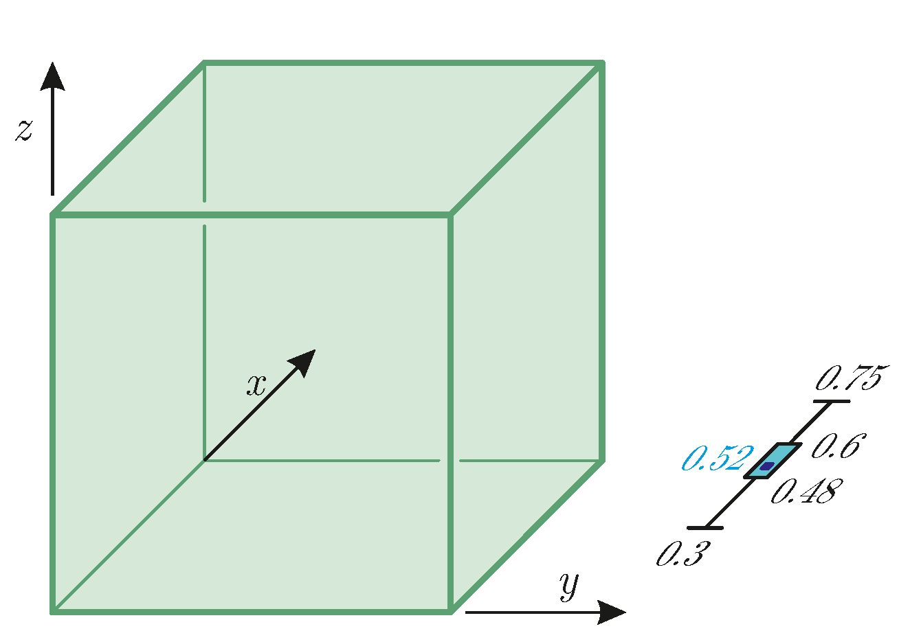
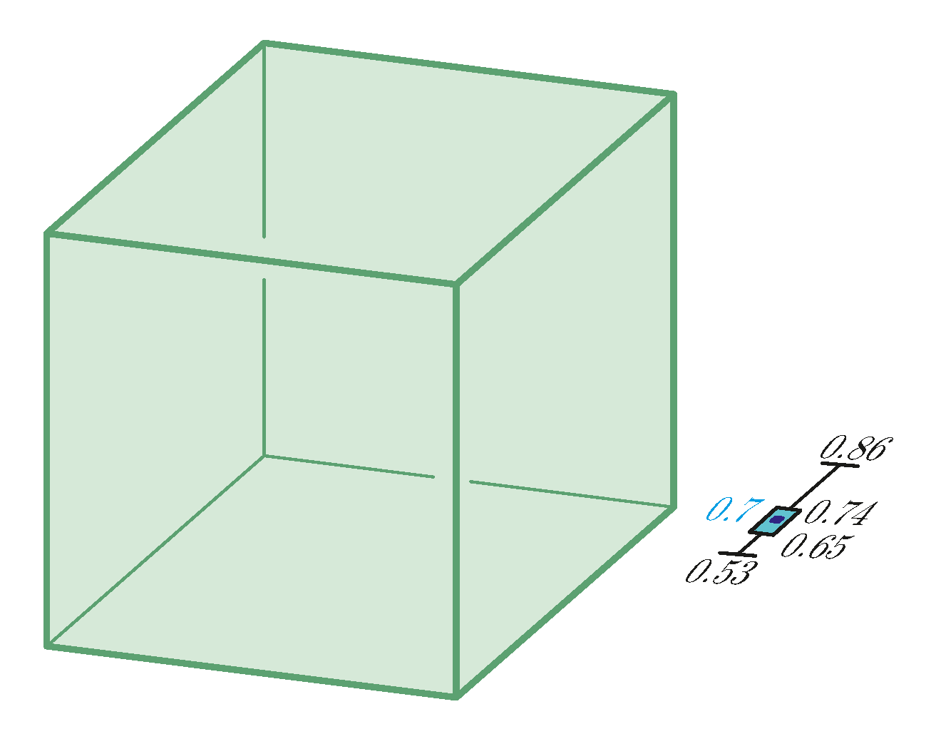
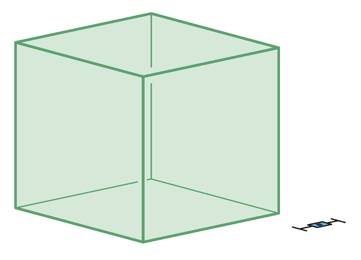
In the first axonometric task, we provided a cuboid in the so-called Cavalier-axonometry: the edges of the cuboid in the
y and
z directions are perpendicular in the image. Students were able to adjust the foreshortening in the third,
x direction. After the evaluation, we found that the mean of the chosen foreshortenings is
, the median value of the answers is
. In
Figure 3, the cube is shown with this latter foreshortening—this is the drawing for which most students believe they see a cube (and not a general cuboid). The engineering convention is
.
On the right side of the figure, the box-plot of the most important foreshortening test data has been displayed as well:
of the responses are in the range
, which is its interquartile range or IQR (green rectangle parallel to axis
x). This is a remarkably narrow interval. The so-called non-outlier range is
. This range contains most of the participants. The remaining few results are the extremes, which will be discussed in
Section 4.3.
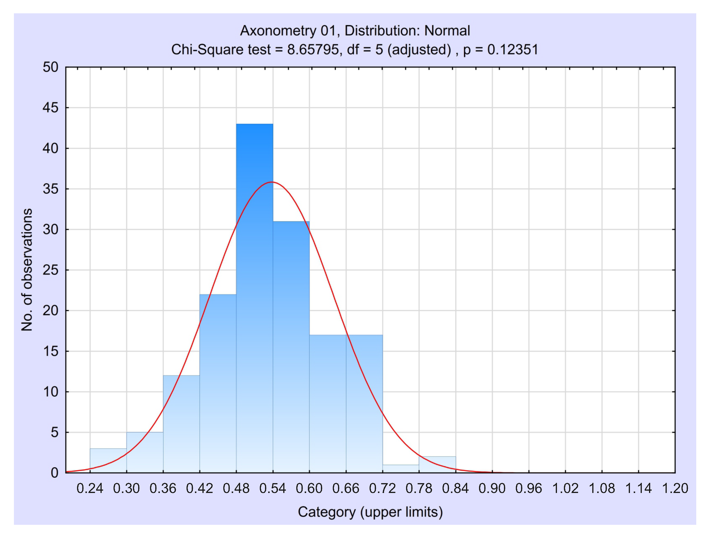
We have also evaluated the distribution of the variable of foreshortening, and we found that it follows a normal distribution (see
Figure 4). This is typical in all the other cases as well.
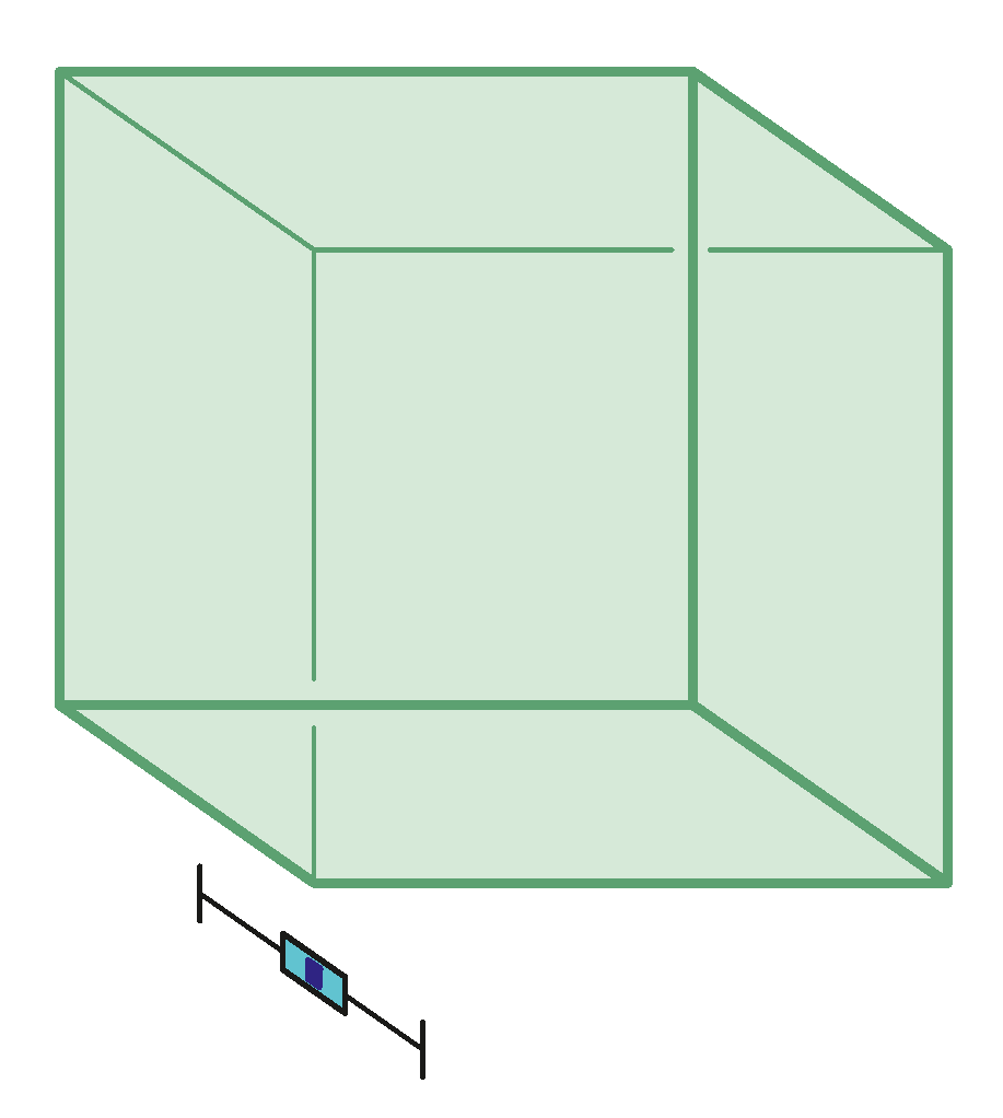
In the following four figures (
Figure 5,
Figure 6,
Figure 7 and
Figure 8), we provide analogous data and views of further axonometric tasks. Data are also summarised for the axonometric tasks in
Table 2, where the conventional foreshortenings are also presented in the first row.
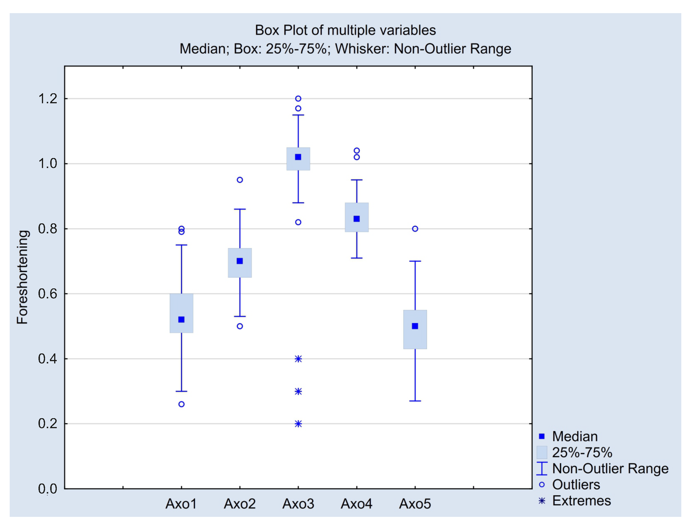
Box-plots of the axonometric test figures are also provided separately in
Figure 9. Here we highlighted the mild outlier and extreme outlier values as well. For example, in the case of the third axonometric task, there were two upper outliers and one under the outlier (small circles). They are farther from the boundaries of IQR than
of the length of IQR but do not go farther than
. Moreover, we found that few students provided extreme values, which will be discussed in
Section 4.3.
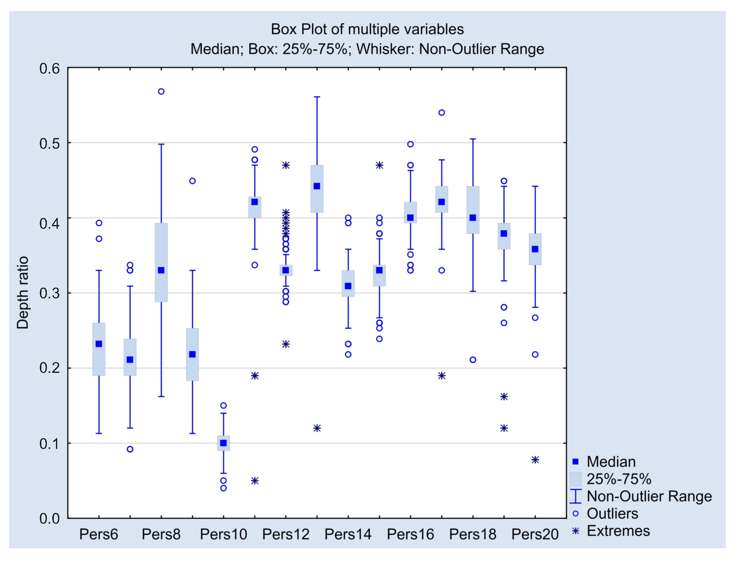
4.2. Perspective Test Results
Students received 5-5 tasks of one-point, two-point, and three-point perspective drawing, separately. Let , , be the unit points, , , be the vanishing points of x, y and z axes, respectively, while the origin is denoted by O. always exists (i.e., it is in finite position); therefore, we can compute the so-called depth ratio (briefly depth) , of the perspective image cube along the x-axis by the ratio of the edge length of direction x of the cube and the distance of the origin and the vanishing point . In the case of two- and three-point perspectives, one can analogously calculate the depth ratio along the other two axes by and, in the case of the three-point perspective, .
In our survey, the only point that the students were able to adjust was
, thus automatically changing the depth ratio
. We restricted the value of
to the range
(only in the case of Pers10 to
). Just as in the case of axonometric tasks, we transformed this depth ratio to a parameter
, and from GeoGebra we received the value
s of the chosen length of the edge in the following form:
The inverse function is . (In the case of Pers10, we have and .)
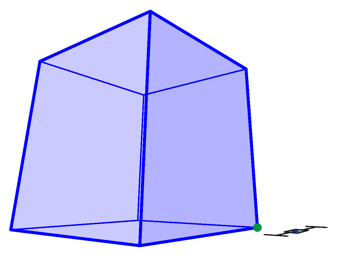
4.2.1. One-Point Perspective Test
In the five tasks of one-point perspective drawings, students were able to adjust point
and thus the depth ratio along the
x axis. As we have discussed above, the crucial difference between the one-point perspective and other perspectives is that here there is not any convention of depth ratio nor a single correct value from the geometric point of view. This method has been frequently applied from the early Renaissance in classical paintings, such as The Cestello Annunciation by Botticelli, The School of Athens by Raphael, or The Last Supper from Leonardo, just to name a few, but with various shortenings. As a consequence, in
Table 3, where the outcomes of the test of one-point perspectives are summarised, we did not provide any conventional or expected value.
Perhaps this is also the reason why the interval between the non-outlier minimum and maximum is mostly larger in these tasks than in the case of two-point and three-point perspectives, with the only exception of the task “Perspective 10” (fifth one-point perspective), where the only vanishing point
is very far from the origin, consequently the drawing is very close to an axonometric image. The first five plots in
Figure 10 show the box-plots of all the one-point perspective tasks, and the cubes with all the data can be seen in
Figure 11,
Figure 12,
Figure 13,
Figure 14 and
Figure 15.
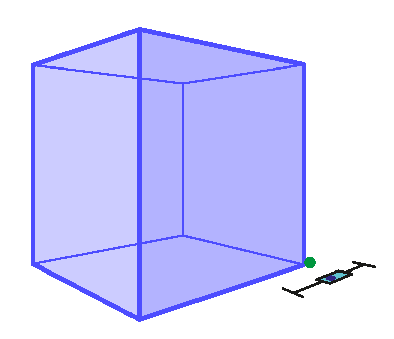
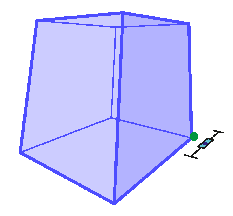
4.2.2. Two-Point Perspective Test
We have provided five different two-point perspective tasks, where, again, students were able to adjust the depth ratio along the
x axis by moving one single point,
. In the case of the two-point perspective, although all figures can be technically correct as a perspective drawing, there is one single solution where the drawing can be a result of a central projection, due to Stiefel [
19]. This single solution is presented in the figures as point
G (green), and the associated depth ratio is listed in the first row of
Table 4, as the expected value.
It is worth noting that in this perspective method, the expected (optimal) value and the mean value of the depth ratio are fairly different in three out of five tasks with very small standard deviation. This means that the depth ratio seems to tendentiously be over or underestimated in some cases by most of the particpants (see the position of the green dot in the figures).
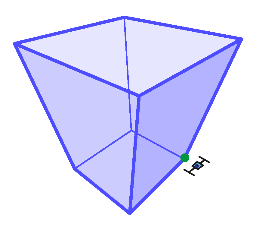
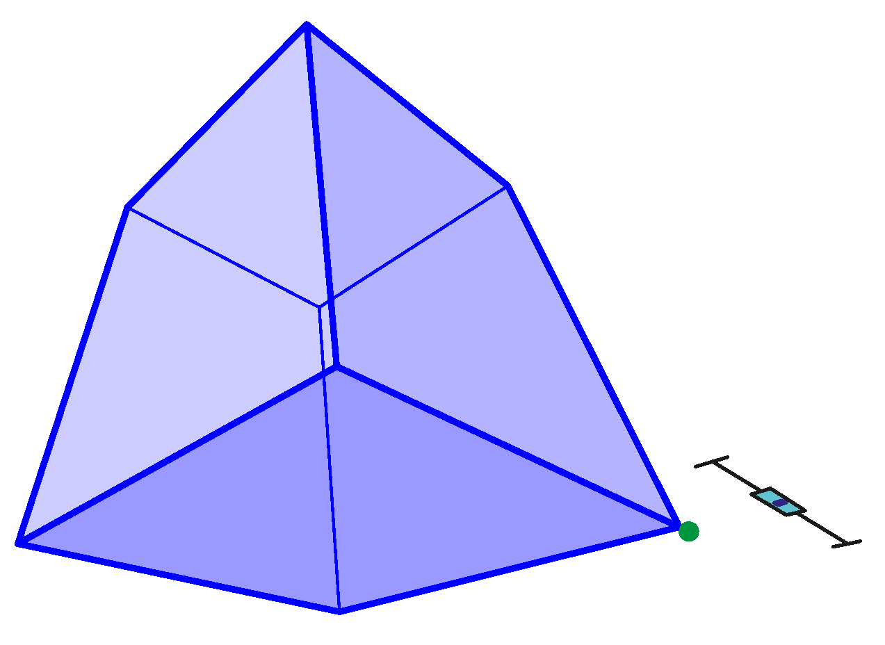
4.2.3. Three-Point Perspective
Analogously to the previous task groups, in this part of the test, five different three-point perspective drawings were provided, and the students were able to adjust the depth ratio along the
x axis by moving point
. In the three-point perspective drawing, similarly to the two-point case, there is a single position of
(and single value of depth ratio), where the image can be considered as a central projection of a cube. This somewhat optimal position of
is denoted in the figures by a green dot. Data of these tasks can be seen in
Table 5, with that single depth ratio as the expected value.
Note that—contrary to what we have observed in the two-point case—in the three-point perspective tasks, there is a remarkable coincidence between the optimal (expected) value of depth ratio and the mean value of the test results. This is also obvious from
Figure 21,
Figure 22,
Figure 23,
Figure 24 and
Figure 25 where the three-point perspective tasks can be seen with the optimal position of the green point. Box plots can also be seen in these figures as well as in
Figure 10 (third group of 5 plots).
4.3. Cluster Analysis
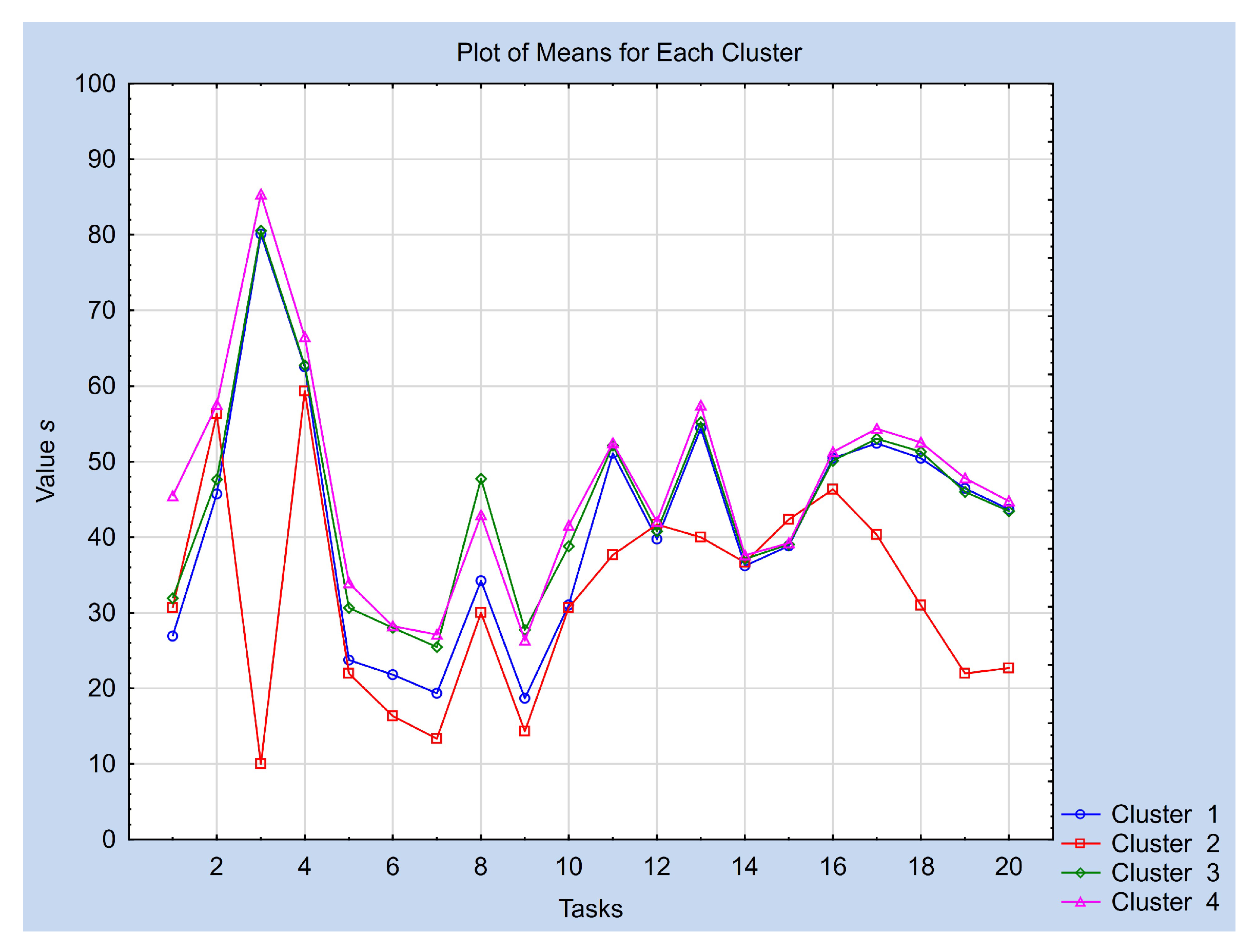
Five-five tasks of axonometric, one-point perspective, two-point perspective and three-point perspective drawings in this order have been provided to the test participants (students of arts and engineering) to find the common sense, if it exists, of seeing a cube (and not a general cuboid). Most students found their best view and foreshortening in a remarkably narrow interval, with small deviation, confirming that there is such a common view. However, different additional lessons learnt from each type of task were provided. We sorted the students into four clusters by the software Statistica, and we found that the results of the students in three clusters differ slightly, while the fourth cluster is spectacularly and significantly different from the other three (see
Figure 26). Cluster 2 contains only three engineering students out of 153. The values sent by them are extremes, as perhaps they did not understand the task or they have slightly different spatial abilities than the majority. The numbers of the members of the other three clusters, Cluster 1, Cluster 3 and Cluster 4, are 61, 45 and 44, respectively. The ratios of the arts and engineering students in the clusters, respectively, are 75–25%, 87–13% and 48–52%, while this ratio in the case of all the students is 70–30%. We found that there is only a slight difference considering Cluster 1, Cluster 3 and Cluster 4 in one-point perspectives, but Cluster 2 has a relevant difference from the others in most of the tasks.
5. Conclusions
In the case of axonometry, every geometrically correct drawing can be considered as a projected image of a cube; therefore, there is no absolute, single right solution. However, in many axonometric situations, there is a kind of convention for the value of foreshortening, inherited mostly from engineering applications. The results of our survey, where students were not aware of these conventions, show that the mean value of the test results is very close to these conventions in most cases, somewhat confirming their existence. One important exception is the task Axo02, a frequently used axonometric framework, where the usual foreshortening is , but the mean and median of the responses are . This fact may raise the possibility of changing the convention in education in this specific case.
In the case of one-point perspective drawing tasks, analogously to axonometry, every geometrically correct drawing can be considered as a projected image of a cube, but in this case, there is no such convention. Among the perspective drawings, these one-point perspective tasks resulted in the largest interquartile and full range, showing a kind of uncertainty about this view.
In the case of two-point perspective drawing tasks, the depth ratio has been chosen from a much smaller interval but with a definite over- or underestimation compared to the single correct geometric solution where these drawings can be considered as a central projected image of a cube.
Finally, in the case of the three-point perspective drawing tasks, having received the same small interquartile range as in the previous case, the mean was very close to the single correct geometric solution. It seems to us that this view, which is the one closest to our everyday life experience, provided the most obvious outcome in terms of common view.
Our experience can be concluded as follows: the perspective and axonometric drawing of cuboids in math textbooks and lessons yield a deeply congruent common understanding in most cases. This especially holds for two-point and three-point perspective representations of which students evidently have a greater everyday experience because they are used to seeing representations of cubes mostly with those dimensions. However, potential reasons of congruent views as well as deviations and discrepancies need further elaboration.
All of this means that when we intend to draw a cube (and not a cuboid), we must take into account this common sense, otherwise students will have a feeling of seeing a general cuboid, and not a cube.
However, as we can observe from the box plots and statistical data of the test results, there is a small group of students, whose results are significantly and consistently different from the others. These students evidently have a very different view of space and suffer from a serious lack of spatial abilities. The study of potential reasons for this difference goes beyond the scope of this paper but can be the subject of future investigations. In a future extended research, we are planning to study whether there is any difference in the perception of the “common sense of cube” in terms of movement type, spatial abilities, age or gender, analogously to what has been reported in perception and spatial abilities in [
20,
21,
22,
23,
24].


