Article

Scanning Signatures: A Graph Theoretical Model to Represent Visual Scanning Processes and A Proof of Concept Study in Biology Education

by
Enrique Garcia Moreno-Esteva
*,
Anttoni Kervinen
,
Markku S. Hannula
and
Anna Uitto
Faculty of Educational Sciences, University of Helsinki, 00014 Helsinki, Finland
*
Author to whom correspondence should be addressed.
Educ. Sci. 2020, 10(5), 141; https://doi.org/10.3390/educsci10050141
Submission received: 28 January 2020 / Revised: 8 May 2020 / Accepted: 11 May 2020 / Published: 15 May 2020
(This article belongs to the Special Issue Networks Applied in Science Education Research)

Abstract

:
In this article we discuss, as a proof of concept, how a network model can be used to analyse gaze tracking data coming from a preliminary experiment carried out in a biodiversity education research project. We discuss the network model, a simple directed graph, used to represent the gaze tracking data in a way that is meaningful for the study of students’ biodiversity observations. Our network model can be thought of as a scanning signature of how a subject visually scans a scene. We provide a couple of examples of how it can be used to investigate the personal identification processes of a biologist and non-biologist when they are carrying out a task concerning the observation of species-specific characteristics of two bird species in the context of biology education research. We suggest that a scanning signature can be effectively used to compare the competencies of different persons and groups of people when they are making observations on specific areas of interests.

1. Introduction

Eye tracking provides a continuous measure for the study of the learning process as it happens, providing a peek into the cognitive processes of the learning subject [1,2]. In education, mobile gaze tracking allows the researcher the possibility of finding out where a student’s visual attention is located while learning [3,4]. However, the synthesis of gaze tracking data is complex. The aim of this paper is to describe a method, based on networks (mathematically speaking, graphs), to make a synthetical description of gaze tracking data with a component synthesizing of the temporal dimension of the data. The method enables a comparison of gaze tracking data coming from different subjects in the context of a common perceptual processes. It is more broadly useful to identify different attentional signatures in data consisting of categorical sequences by inspection, or quantitatively as well. In our model, the uniformity or lack of uniformity in the weights of the edges of a network, represented as the width of the edges, and the order of the edges, represented by the color of the edges, allows for a qualitative or quantitative inspection of the data and the detection of possible cognitive processes at work. To show how this can be so, we present a proof of concept study involving two participants. Since this is a proof of concept study, the small number of participants is of no consequence. The study is meant to illustrate the power of the method.
Representing gaze tracking data in a meaningful way is difficult because the raw data is very rich in information. When we scan a scene, our eyes focus momentarily on a spot—a fixation—and then move rapidly to focus on another spot—a saccade [5]. Frequently, gaze tracking data is annotated in terms of gaze targets or areas of interest (AOIs), specific regions in the scene upon which the subject wearing the gaze tracking device is looking. The period of time during which the focus of the eyes remains on a specific AOI is called a dwell. Annotations can be done manually or with the aid of an automatic fixation detector.
There are established methods to capture the essence of a visual scanning process, for example, heat maps or dot plots [6], but these methods provide no information about the temporal dimension of the gaze behavior. The use of graphs and networks is not new in gaze tracking (in education research, c.f. [7]), but the synthetic representation of temporal information in our model is. The temporal dimension of gaze behavior is typically included in the scanpath, i.e., the sequence of fixations or AOIs. Anderson et al. [8] review various methods for comparing scanpaths. Many of these methods [7,9,10] exclude the temporal dimension. On the other hand, those that include the temporal dimension fail to make a concise synthesis of the gaze process, i.e., they preserve too much of the information, thus making interpretation of results difficult.
As it is argued in [11], the temporal aspect of a perceptual process is crucial for its adequate identification and in the comparison of several such processes. However the method in [11] is most suitable for the analysis of raw fixation scanpath data (coordinate sequences), rather than categorically annotated data (AOI sequences), even if some attempt is made to simplify the information of the scanpaths (the data they consider). Moreover, their method is meant to work with shorter visualization processes. The temporal information of the scanpath is used, but it is not synthesized concisely and in such a way that the order in which events unfold can be compared by inspection.
Our method uses annotated dwells on areas of interest (AOIs) and is thus one step removed from the raw fixation and saccade sequences used in [11]. Our method can be modified to be used with annotated fixations, as we will describe when discussing variations of the method. In fact, our method will work with any data that can be represented as a sequence of categories. Our method has no limitation on the number of AOIs or the length of the episode. We argue that for gazing events lasting several minutes, our representation is simpler, and also much more informative and useful for making comparisons between different visualization processes than any of the previously published methods. The core purpose of our method is to summarize complex data in an easily digestible form so that different processes can be compared by inspection through a pictorial representation. Moreover, our method provides meaningful and robust quantitative variables of gaze data, making it easy to continue with statistical or machine learning analyses.
According to the eye-mind hypothesis, eye movements relate to the cognitive process of a person, suggesting that the direction of human gaze and the focus of attention are connected [12]. Moreover, visual attention can indicate levels of competence in intellectual tasks. Thus, understanding what a person pays attention to in a cognitive task such as a recognition, identification, or classification, allows the researcher to better understand the task solving process [13].
In science education, precise observations of the environment and natural phenomena are at the foundation of meaningful and successful learning experiences [14]. However, making relevant observations and learning from them is not an easy task. Studies have shown that students may easily fail to learn from demonstrations [15], or that making observations even in authentic research contexts might not help students to learn [16]. In biology education, one learning objective for the secondary school curriculum in Finland is the basic skill of identifying the most common species of the nearby environment (e.g., plants, animals, mushrooms, see Finnish National Board of Education, [17]). However, in spite of educational efforts, primary and secondary school students’ as well as teacher students’ species recognition and identification skills have remained low [18,19]. Thus, to develop biology education, teachers’ and students’ knowledge about species, and their skills to make biodiversity observations, should be better understood. In this article we present a proof of concept study involving only two participants illustrating how our method helps analyze and understand an obervational task in educational biology. Since this is a proof of concept study, the number of participants is of no consequence.
This study is carried out as part of the research project “Biodiversity for Science and Sustainability Education” (BSSE), in collaboration with the research project “Mobile Gaze Tracking for the Study of Attention and Emotion in Collaborative Mathematical Problem-Solving” (MathTrack), both from the University of Helsinki.

2. Methods: Construction of the Network Model

The aim of the data collection was to experiment with technical and methodological applications of mobile gaze tracking to biodiversity education research by studying perceptual performance when making observations of birds. In the experiment, the use of visual markers (see, e.g., Figure 1) for automatic AOI recognition was also tested, but that data is not reported in this study.
In order to study observations two participants were equipped with mobile gaze trackers [4] which record the gaze video allowing the researchers to see what the subjects paid attention to as they scan the scene. The setup consisted of two different bird species, the short eared owl (Asio flammeus) and the curlew (Numenius arquata); see Figure 1. Some features of the bird species are known to indicate adaptation to very different food sources and habitat. The test topic of the experiment, identification of the general features of the biological adaptation of the species, is key content in secondary school biology education (e.g., [17]).
Because of the experimental and technical purposes of the study, two of the authors of this study were also the test subjects (TS1 and TS2) wearing the gaze tracking devices. The test subjects were asked to look at the birds and compare their characteristics, and to think aloud how the birds might have adapted to their environments.
Because of a different educational background of the test subjects (biology and mathematics) we could only assume that their perceptual task performance might differ. In particular, we thought that the biologically trained subject would exhibit a more focused gazing behavior, something that becomes evident in the results presented in Section 3. This study was carried out to develop and test the data collection and analysis methods, and find out whether mobile gaze tracking can be used to study observational processes in biology education. For the gaze tracking data collected, we wanted to obtain a representation (the network model) which could be used to represent the gaze patterns of the test subjects in such a way that they could be meaningfully compared. The recording of the gaze videos lasted 2’40” for TS1 and 1’50” for TS2.

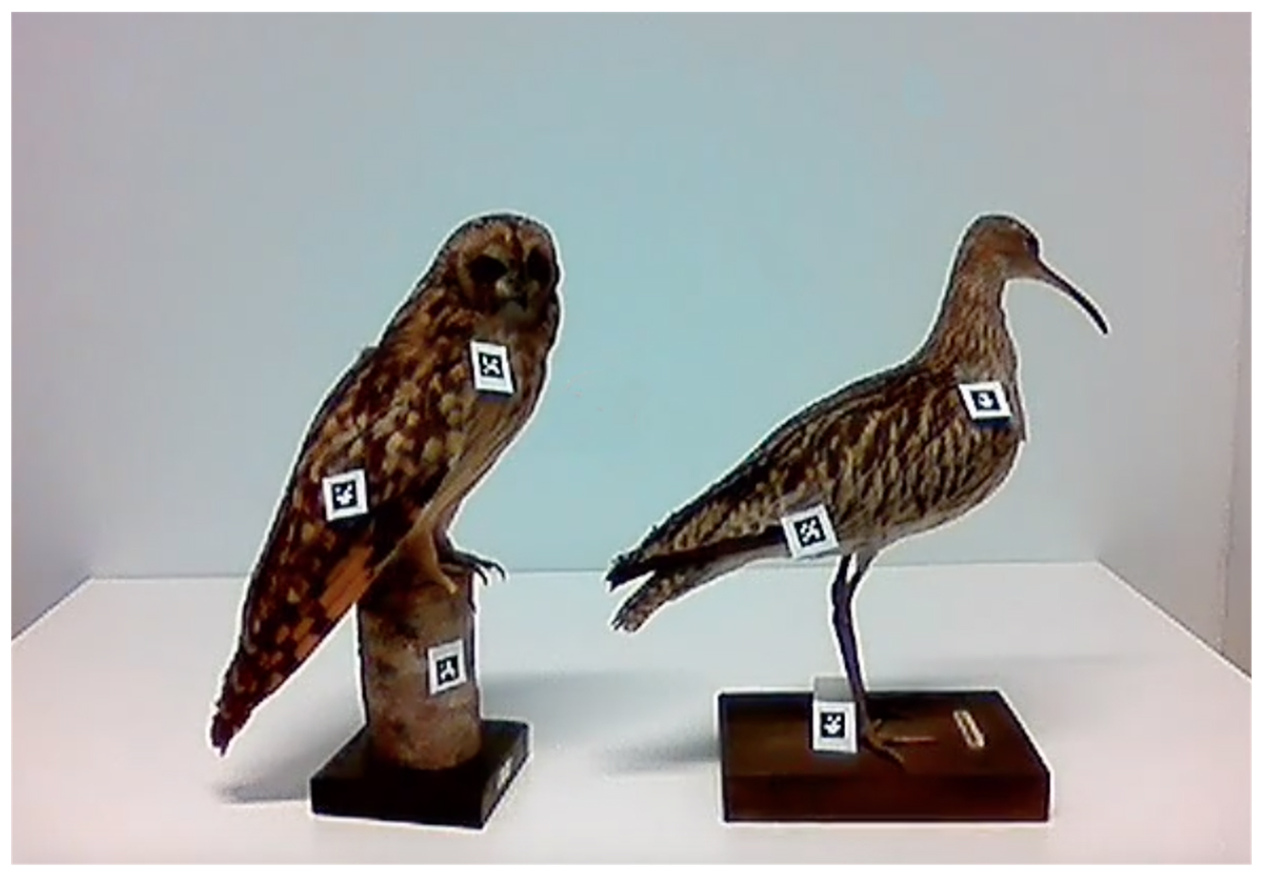
2.1. Data: Gathering and Preparation

The data obtained from the gaze tracking devices is a video of the scene observed by the subject wearing the glasses, together with a red dot on the spot where the subject’s eyes were focused. We annotated dwell AOIs in our videos manually.
The AOI were six anatomical structures for each bird, each of which was coded with a number: Beak (2 and 8), chest (5 and 11), wing (4 and 10), head (1 and 7), tail (6 and 12), and feet (toes 3 and 9). Code number 13 was used to represent dwells on areas which are not of special relevance to the task (blank areas). See Figure 2.
After annotation, each data item becomes a sequence of annotated dwells, with each pair of consecutive dwells having a different annotation, that is, representing different AOIs. In this form, the data looks like a sequence of number pairs ( u , t ) , where u is the code of an AOI and t is a number representing time, the duration of the dwell. We did not use the duration of the dwell information, so that our sequence ended up being just a sequence of AOI code numbers.

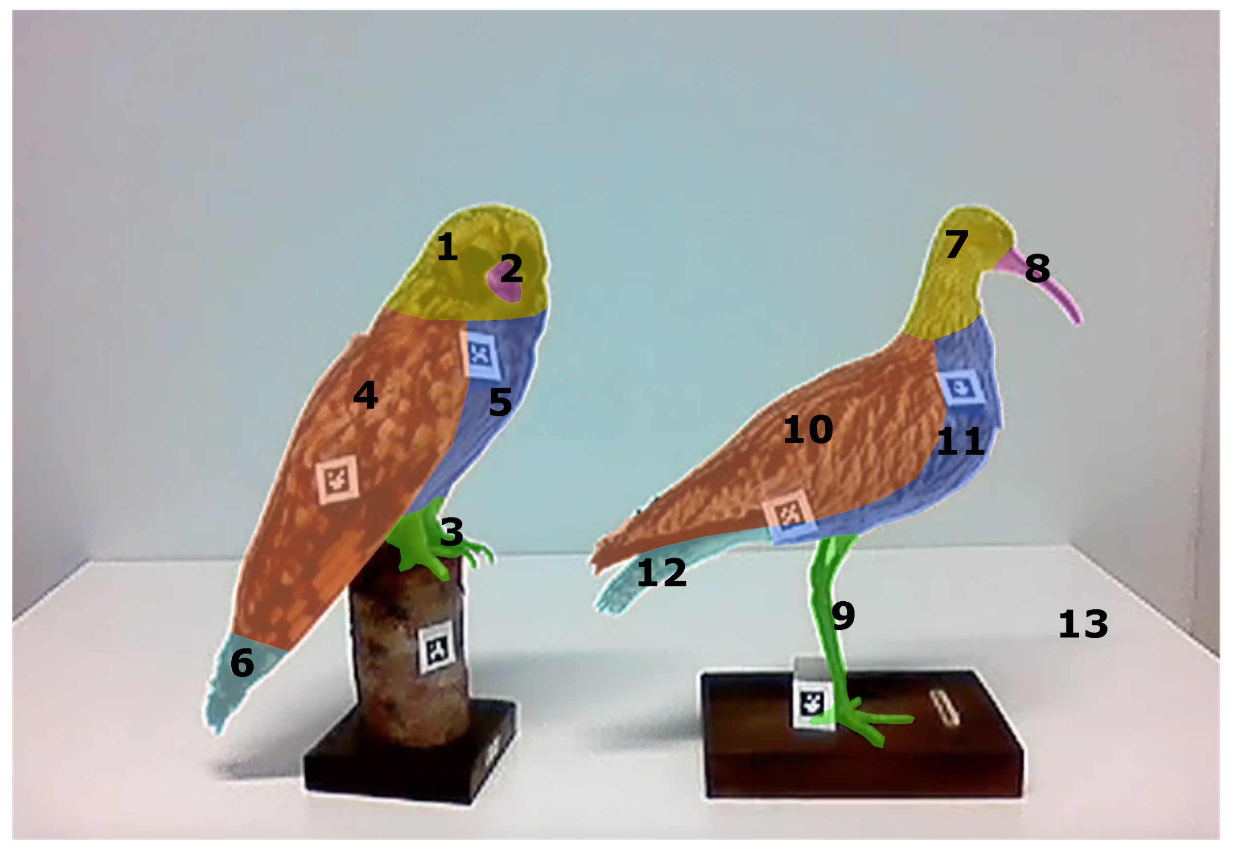
2.2. Basic Definitions and Idealizations

The starting point for describing our model are the sequences of AOI code numbers that we described in the preceding section. To describe our method we use the terminology of graph theory [20] —in graph theory parlance, networks are called graphs, and nodes are called vertices. A sequence of AOI code numbers can easily be represented as a graph as follows. The vertices of our graph are the different AOIs, each represented by a unique number. Our graph is given by a set of n vertices (in this case n = 13 ), each vertex represented by one of the first n numbers, and by arcs (some use the term directed edges) between two vertices that correspond to codes that appear consecutively in our sequence of codes; in our initial model, we put one arc for each pair or consecutive codes, so that there may be multiple instances of an arc if a pair of codes appears consecutively many times in the code sequence. This kind of a graph is called a directed multigraph.
From the sequence of codes we obtain a sequence of vertices and arcs which alternate, something which in graph theoretical terms is called a directed walk. With all this done, we already have a “network model” of our data sequence, the directed multigraph together with the directed walk. It is important to notice that the directed multigraph we have obtained, together with the directed walk, contain exactly the same information as our sequence of AOI code numbers. In order to carry on with our analyses, we need to simplilfy things further without losing too much information.
We will introduce some notation and terminology for the sake of simplifying the ensuing discussion. We will call our sequence of gaze target codes S. The directed multigraph we obtain from it is denoted by M. The set of vertices of M will be denoted by V ( M ) or V if it is clear what graph this set refers to, and A ( M ) will denote the set of arcs (similarly, A). The number of nodes in V ( M ) is called the order of M and it will usually be denoted by o or o ( M ) , and the number of arcs is called the size of M and it will usually be denoted by s or s ( M ) . The walk we obtain from S will be denoted by X S (we are reserving the use of the letter W for another purpose). As remarked above, our directed walk (which is defined in terms of the multigraph) essentially contains the same information than our sequence of gaze target codes. The number of instances of a particular arc in M is called the multiplicity of the arc in M, and if a is an arc, we will denote the multiplicity of a by m ( a ) . This number is the same as the number of times that a given arc appears in the directed walk X S .
The reader can consult [20] to learn about graphs and networks. We note that in mathematics, networks are usually called graphs. In some other fields, the term network is preferred. We will use the mathematical convention and call our models graphs rather than networks.
Directed walks surely are useful, but if, like in our gaze tracking derived gaze target code sequences, there are relatively few nodes compared to the number of arcs, so that some arcs occur with great multiplicity, the model can be simplified substantially if we can manage to get a graph in which each arc occurs only once. The key thing is that we can still define our walk in this new graph. Ultimately, we will want to use the new graph for the analyses rather than the walk, the former being a lot simpler and being subject to analyses which are more easily made in terms of the graph than in terms of the walk. The new graph will provide a rich synthesis of the information contained in the walk.
The idea is to make a simplification which retains essential information about our original graph. This can be done if
  • we keep a record of how many instances or occurrences there are of each arc,
  • if we keep a record of how many times a vertex is “visited” in our walk,
  • and if we keep information about the order in which arcs are traversed along our walk in some way.
When we move on to our applications and analyses sections, we will illustrate the usefulness of our simplified graph and model, and we will argue that these three book keeping procedures together with the graph itself are like a fingerprint of the process that we are trying to model and which can be analyzed in a variety of ways, including qualitatively. We will call our final model a scanning signature of the AOI code number sequence. Let us formally define some of these things so that they have a quantitative and precise meaning.

2.3. Arc and Vertex Weights

We start by describing how we add a little bit of information to a simplified graph in which each arc is represented only once, but so that it is able to tell us most of the story that our walk tells us. Recall that the walk contains essentially all the information that our code sequence contains. The multigraph we obtained from the walk is called M. We obtain a new simple graph (to which we will refer to simply as graph) G from M by removing multiple instances of the arcs in M. Having only one instance of an arc allows us to define an arc formally as an ordered pair ( u , v ) of vertices u and v. For the formal definition of a directed multigraph, see for example [21]. Note that V ( G ) = V ( M ) but that A ( G ) A ( M ) . To compensate for the loss of information due to the removal of multiple instances of our arcs, we associate to each arc in G a weight via a function W A : A ( G ) [ 0 , 1 ] . If an arc a appears m ( a ) times in the directed walk that was obtained from the code sequence, that is, if its multiplicity in M is m ( a ) , then its weight is W A ( a ) = m ( a ) / m A , where m A is the largest number of times any arc appears in our directed walk, that is, it is the largest multiplicity among the multiplicities of all the arcs in M. Please note that the size of G or number of arcs in G is most likely different than the number of arcs in M by virtue of the fact that in G, the multiplicity of each arc is 1.
Similarly, we will associate a weight to each vertex of G defined by means of a function W V : V ( G ) [ 0 , 1 ] . For a given vertex v, if this vertex appears x times in the code sequence which we used to define the graph, then W V ( v ) = x / m V , where m V is the largest number of times any vertex appears in our code sequence.
If we were to represent the weights of the vertices and arcs pictorially by circles of a given maximum radius and arrows of a maximum thickness, the size of the vertices and the thickness of the arcs in a pictorial representation of G would be proportional to their weights relative to this maximum radius and thickness. Note that the weight of the vertices is proportional to their radius rather than the area of the circles which represent them. This is because the size of a circle is normally perceived to be proportional to its linear rather than to its quadratic dimensions. It is also the way that computer languages implement the relative size of pictorial objects.

Average and Idealized Position of An Arc, and Idealized Walk Sets

So far we have not synthesized the temporal order of arcs in the directed multigraph. In order to do away with our data sequence and directed walk entirely, we need to somehow capture the essential story which the order of appearance of the arcs in the sequence of arcs in the directed walk is telling us. To do this, we compute the average position of an arc in the original directed walk arc sequence. We note the positions in the arc sequence of the directed walk in which a specific arc occurs. We then take the average of these positions (we add the position numbers and divide by the total number of occurrences of the arc), and we further divide this number by the total number of arcs in the directed walk or in the original graph M. The resulting number is a number between 0 and 1. We asssociate with each arc in G, this number. We will let P μ : A [ 0 , 1 ] be the function which associates this number to each arc. If we then sort the average positions of the arcs from smallest to largest, we get a new ordering for the arcs. The order of an arc in this new ordering is the idealized position number of an arc in G. (note: If two (or more) arcs have the same average position, we sort those arcs lexicographically). We shall let W P : A { 1 , , s ( G ) } be the function which associates with each arc its idealized position number. The sequence of arcs in the order of their idealized position we shall call the idealized arc sequence of G and the order of the arcs given by their ideal position is called the ideal order of the arcs in the scanning signature. With this idealized order information given, we can do away with our original data sequence.
In our pictorial representation of G the idealized position number will be given by the color of the arc, understanding that the progression of colors is given by the hue in increasing order, starting with red, and following by orange, yellow, green, light blue, dark blue, and purple shades of colors.
Summarizing, our graph G together with the weight functions, the average position function, and the ideal position function are a scanning signature of our code data sequence. For each AOI, we identify how often it is looked at, giving rise to the weight of the corresponding vertex. For each arc between two AOIs we identify how often that transition is made, which gives rise to the weight of the arc; we see how early or late these transitions on average appear, which gives rise to the average position of the arc, and in turn gives rise to a new ordering of the arcs.

2.4. Comparability of Graphs Obtained from Different Data Sequences

One advantage of our final graph representation is that graphs obtained from different data sequences are similar in that they have the same sets of arcs. Only the weight functions may be different. Essentially, to insure that all graphs have the same set of arcs, we include arcs that are not present in the original directed walk, but we give them an arc weight of 0. However, the length of the idealized arc sequence includes only arcs that are used in the original walk and that do not have a weight of 0 in the scanning signature. In our pictorial display of these graphs we only show arcs that do not have a weight of 0. In practice, this suffices to make a qualitative distinction among different data sets.
Our graph model makes it possible to compare these various graphs mathematically with all kinds of tools, whether they be statistical, algorithmic (as with machine learning techniques), or otherwise graph related measures. In what follows we will illustrate some such type of analysis which can be done with statistics, and which, in fact, is visible to the naked eye from the pictorial representations.

3. Results: A Proof of Concept

We now look at a specific example. We look at the gaze sequence of the two participants obtained during their observation of the two birds.

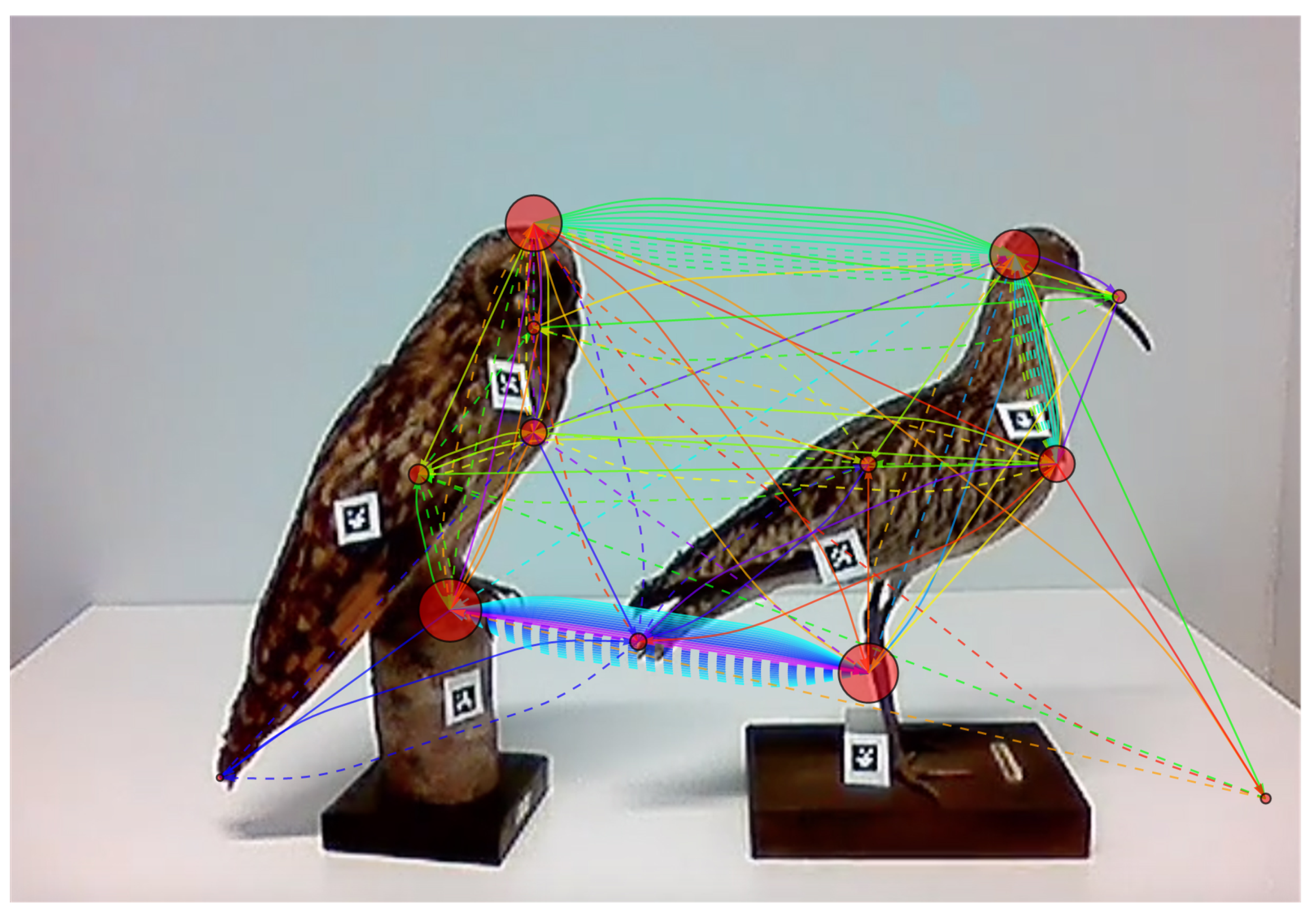
3.1. The Constructed Network, a Scanning Signature

The data sequence in our example is an AOI code sequence obtained from TS1, a test subject with training in biology, who was asked to scan the scene and look for features in the animals that indicate an adaptation of the animal to its habitat. From the following sequence
S 1 = { 11 , 13 , 1 , 11 , 12 , 1 , 9 , 10 , 1 , 2 , 1 , 3 , 5 , 1 , 13 , 3 , 1 , 9 , 7 , 11 , 2 , 8 , 9 , 11 , 5 , 1 , 5 , 4 , 10 , 1 , 4 , 5 , 11 , 7 , 10 , 5 , 11 , 7 , 4 , 11 , 10 , 4 , 3 , 1 , 8 , 2 , 8 , 7 , 13 , 4 , 3 , 4 , 2 , 1 , 7 , 1 , 7 , 1 , 7 , 1 , 7 , 1 , 7 , 1 , 7 , 11 , 7 , 11 , 7 , 11 , 7 , 3 , 9 , 3 , 9 , 3 , 9 , 3 , 9 , 3 , 9 , 7 , 9 , 3 , 9 , 3 , 9 , 3 , 9 , 3 , 9 , 3 , 9 , 3 , 9 , 3 , 6 , 12 , 6 , 5 , 12 , 10 , 12 , 1 , 5 , 7 , 8 , 11 , 12 , 3 , 9 , 5 , 1 , 3 , 9 , 3 , 9 }
we can obtain the multigraph M S 1 in Figure 3 below:
Each vertex corresponds to a number in the sequence and it is shown in a size proportional to the number of times it occurs in the sequence. The color of the arcs indicates the relative order in which they are traversed in the directed walk defined by the sequence. The colors progress from red, to orange, to yellow, to green, to cyan, to light blue, to dark blue, and to purple. The vertices of the graph have been superimposed on the scene AOIs represented by their corresponding AOI code numbers. Part of the directed walk X S 1 is the following:
X S 1 = { 11 13 , 13 1 , 1 11 , 11 12 , 12 1 , 1 9 , 9 10 , 10 1 , 1 2 , 2 1 , 1 3 , 3 5 , 5 1 , 1 13 , 13 3 , 3 1 , 1 9 , 9 7 , 7 11 , 11 2 , 2 8 , 8 9 , 9 11 , , 7 8 , 8 11 , 11 12 , 12 3 , 3 9 , 9 5 , 5 1 , 1 3 , 3 9 , 9 3 , 3 9 }
The scanning signature G S 1 is given in Figure 4 below. Below it in Figure 5 is the scanning signature obtained from another gaze target code sequence, S 2 , obtained from TS2, the test subject with no background in biology.
The two pictures speak for themselves. The pictures suggest the following: The main difference between the two is that in the scanning signature in Figure 4 there are a few (four) relatively thick arcs, and many relatively thin arcs. In the picture in Figure 5 the thickness of the arcs is a lot more even. There are other differences pertaining to the size of the vertices and the relative ideal order in which the arcs were traversed. However, the main difference that we referred to in the sentence before the last is something which can be studied mathematically. It has to do with the uniformity of the distribution of arc weights. It is possible to use tools from statistics to study how well a dataset fits a distribution, in our case, a uniform distribution. The tool of choice is the χ 2 statistic, which for a set A ( G ) of arcs is defined as follows:
χ 2 ( A ( G ) ) = a A ( G ) ( m ( a ) m ¯ ) 2 / m ¯
where m ( a ) is the multiplicity of a in M and m ¯ is the number of arcs in M (that is, the sum of their multiplicities) divided by the number of arcs in G. The same statistic can be obtained from the weights of the arcs in G. Here, we must remember to use 0 as the multiplicity of the arcs in G that are not used in the original directed walk or have weight 0 in G. A lower value of this statistic means our data is “more uniformly” distributed. The arc weights of data from TS2 are more uniformly distributed, so we would expect that the value of this statistic is lower for these data, closer to 0. The simplicity of this analysis illustrates the power of our method. The visual representation of our data already suggests something in particular about it that one can put to the test mathematically.
To make the quantitative analysis above closer to what we get in the picture, we can apply the statistic exclusively to the arcs that are visible rather than to all the arcs. It should still work, especially if it works qualitatively. If there is a qualitative difference, it will already show if the statistic is applied only to the visible arcs. Doing this, in the case of our two examples, we get, for TS1, a value of 173.69, and for TS2, a value of 8.2, with the two values bearing the expected relation.
Based on the mathematical result above, we can speculate about potential explanations for the differences of the subjects’ scanning signatures (in our view, speculating and hypothesizing is an important part of the scientific method when followed by rigorous empirical testing). Test subject TS1 may approach the task knowing what to look for, and not having to “look around” and scan the scene in an apparently random way. Test subject TS2, on the other hand, not having the necessary background knowledge, will ”look around” a lot more rather than not.

3.2. Analyzing the Temporal Dimension

Our model provides even more information than just the weights of different arcs. The outstanding feature of TS1’s scanning signature are the thick arcs between the heads and the feet. It is apparent that for this participant, comparing the heads of the birds first, and then the feet, was the most important component of the task. The color of the arcs tells us in which order these subtasks were carried out.
Let us try to improve our picture of what the two participants are doing. We have thus far only used the vertex and arc weights, but we have not used the ideal position of the arcs. How do they inform our understanding of what the two participants are doing? One such possibility is to study the relative delay with which portions of the task take place. Since our scanning signature gives us a temporal order telling us how important events unfold on average, we can measure, relatively speaking, how long it takes for certain things to happen. The one common feature of TS1’s and TS2’s gaze behavior is that they both compare the feet significantly more than other parts of the body of the birds. Both participants compared the heads of the birds as well, but TS2 did so quite a bit less relative to how much he compares the feet. Test subject TS1 compares the heads almost as much as the feet. We might want to find out how relatively soon, or late, these comparisons take place in the timeframe of the whole scanning process.
We look at the ideal position of the arcs between the feet and the arcs between the head, and we note the total length of the idealized arc sequence. Suppose that in the case of the biologist, the idealized position number of the arc that goes from the head of the owl to the head of the curlew is p S 1 h , suppose that the idealized position number of the arc that goes from the feet of the owl to the feet of the curlew is p S 1 f , and suppose the length of the idealized arc sequence is l S 1 . We then consider the numbers p S 1 h / l S 1 and p S 1 f / l S 1 . These numbers are between 0 and 1, and they tell us, relative to the length of the scanning process, at what moment in that relative timeframe the participants make the head and feet comparisons. Our two pictures indicate (by the color of the pertinent arcs), for example, that the feet were compared at approximately the same time by both participants, in the later stages of the perceptual process, but that TS2 examined the heads early on (before the feet) and late on (after the feet), and as we had noted before, did not pay particular attention to the heads anyway.

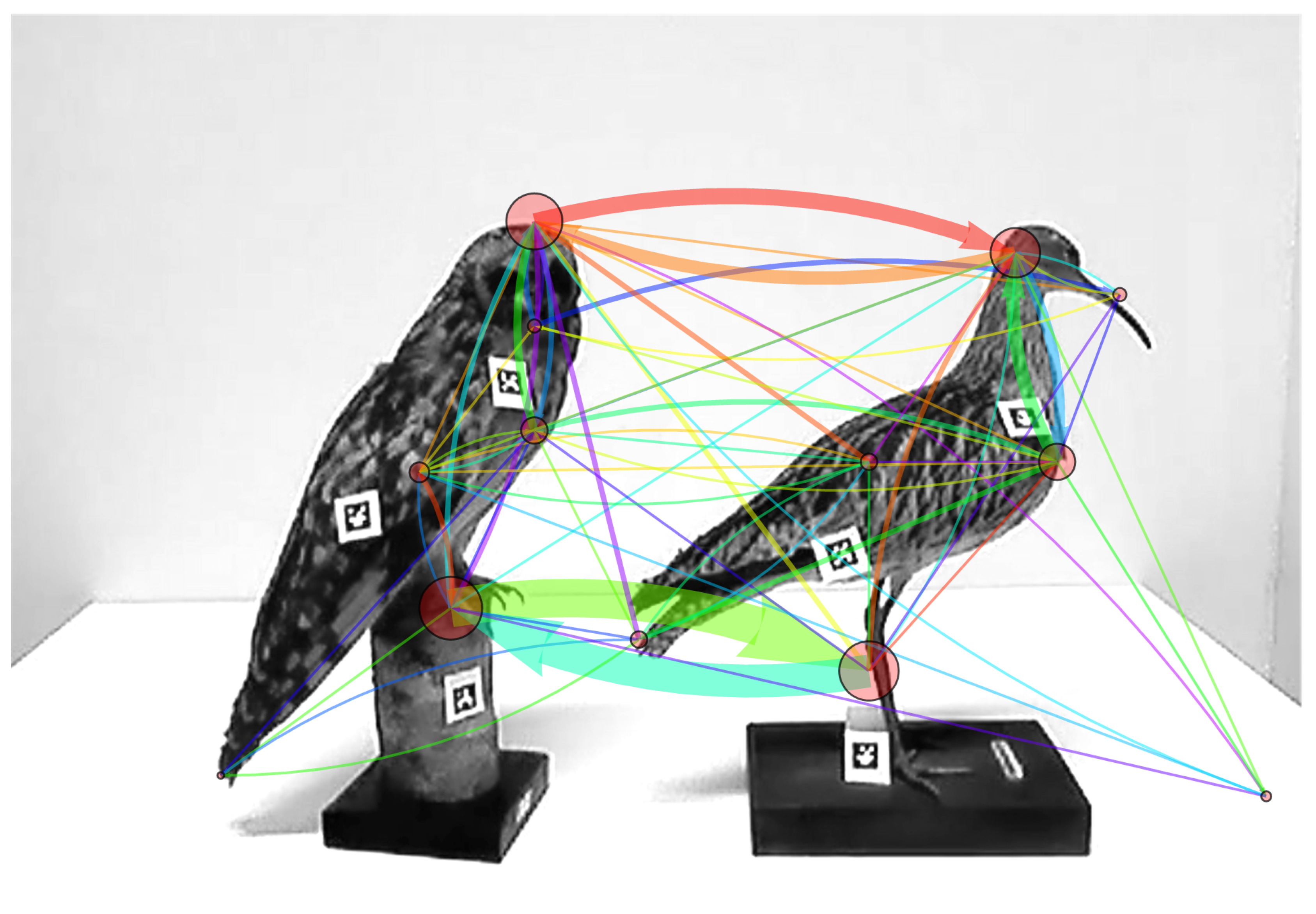
3.3. Comparing and Combining Scanning Signatures

While we have presented data from only two test subjects we could collect and compare similar scanning signatures from a larger group of participants.
The first thing that is important to know is that scanning signatures from different participants or scannning processes are comparable. The weights of the vertices and arcs have been normalized to be a number between 0 and 1, where 1 is attained by the vertices and arcs with highest multiplicity in M S . Hence, it is possible to combine multiple participants’ data into a single scanning signature that is representative of the perceptual strategies of the studied participants. We can combine the data for the weight functions and ideal position functions to obtain a new weight function and ideal position function which describes the combined scanning signature. It is important to remember that the set of arcs of two scanning signatures is the same, if some arcs are not used, they have a weight of 0. The average position of an arc that is not used is a more delicate issue which will be discussed ahead.

3.3.1. Combining Vertex and Arc Weights of Two Sequences into a Single Scanning Signature

The way to calculate the combined weigths of vertices and arcs in two (or more) multigraphs is to add, for each arc (similarly for vertices), the multiplicities of the arcs in the two directed multigraphs from which the individual scanning signatures were obtained, and when that is done, dividing the values obtained by the maximum value obtained for arcs (vertices).

3.3.2. Combining the Temporal Structure of Two Sequences into a Single Scanning Signature

Calculating the average and idealized position of the arcs is a bit more delicate. The calculation involves all the arcs that are used in either of the two scanning signatures. We start by normalizing the positions of the set of arcs of the data set (directed walk or multigraph) which has a fewer number of arcs relative to the number of arcs of the dataset (directed walk or multigraph) which has the most arcs. Let us say that for sequence S 1 there is a multigraph with a total number of k arcs, and that for sequence S 2 there is a multigraph with a total number of l arcs, and suppose that k < l . We would modify the set of arc positions for the multigraph M S 1 by multiplying the position numbers of those arcs by l / k . We would then calculate the average positions for the set of all arcs from both M S 1 (using the modified arc positions) and M S 2 , and from the average positions, the idealized positions. The reader might wonder what happens at this stage with arcs that appear in one multigraph and not in the other. Effectively, what happens with these arcs is tantamount to the statistician’s solution for dealing with missing data by means of replacement with the mean. We omit the technical discussion of this. We want to emphasize that, since there could be potentially many arcs that are not used, we want to restrict scanning signature information to that of arcs which are used, not to the whole set of possible arcs in a complete directed graph (a graph in which all possible arcs are present). Our ability to do this in practice makes our resulting scanning signature qualitatively useful.

4. Discussion and Conclusions

4.1. Extensions of the Model

In this section we provide alternative procedures for the model and extensions of the model.

4.1.1. Using Fixations—Loops and Pseudographs

In our analysis we have used dwells. It would be possible to use fixations instead of dwells. In this case, there might appear multiple consecutive fixations in the same AOI. These can be handled as loops in a type of graph called pseudomultigraph. With this graph all the analyses we have described can be carried out as with a multigraph, and from it, it is possible to obtain a simple pseudograph.

4.1.2. Combining the Data from Many Scanning Signatures and Using It as a Combined Signature

We are now ready to combine many scanning signatures. The averaging procedures described in the preceding section are applied to a whole set of data, multigraphs, or scanning signatures that we might have.
Combining many sets of data into one scanning signature might be desirable, for example, if we have cohorts of experts and novices whose perceptual processes we wish to compare, given a hypothesis that they would differ. Do the combined scanning signatures reveal features that are outstanding in different types of gaze patterns, for instance, the gaze patterns of expert biologists and more novice students? Do they look similar, do their temporal structures look similar?

4.1.3. Vertex Weights

It is possible to use the temporal duration of each dwell or fixation to calculate a weight for the vertex which is proportional to the total amount of time spent on each AOI. These weights are also informative in a different way and the research question would determine which type of vertex weight is more appropriate.

4.1.4. Temporal Information for the Vertices

It is posible to calculate average position and idealized positions for vertices. The resulting information is an abstraction of the order in which target areas were visited. The procedure for calculating this information is analogous to that of the arcs. In a pictorial representation, color could be used for the vertices to represent the ideal order in which they were visited.

4.1.5. Standard Deviations besides Means in the Temporal Information of Arcs and Vertices

In addition to the average weight and position, it is possible to compute also a standard deviation, making it possible to use standard parametric statistical methods to analyze the graphs in detail.

4.2. Conclusions and Directions for Future Work

We have described a network model that promises to be very useful in analyzing gaze tracking data in educational research. For annotated dwell sequences involving a fixed scene and which last a few minutes, it seems to provide excellent results and allows the easy comparison of perceptual processes from different participants. Moreover, our model provides a synthetic description of the temporal order in the sequence of perceptual events, something which for many authors (e.g., [11]) is critical in the proper classification and identification of gaze tracking data.
Drawing from a case from a biology education context, we have shown how scanning signatures obtained from gaze tracking measurements might be a useful tool for analyzing the perceptual performance of different persons. We have shown how the scanning signatures can be interpreted in a way that correlates with the level of expertise of the participants. In science education, learning about scientific phenomena often requires observations or inquiries of the surrounding world or an experiment; thus, the complex perceptual process of observation not only grants, but also requires specific conceptual disciplinary knowledge [14]. Future studies may show how scanning signatures may be used to study the role of the conceptual knowledge and perceptual skills, for instance, when teachers and students make observations in biology.
Moreover, there are many areas of eye tracking research where the temporal dimension of a perceptual process is important. In general, the scanning signature would be a useful method to analyze gaze tracking data from as diverse fields as from radiology and nursing, marketing research, and education; data with user interfaces and web platforms, such as online courses and webpage navigation data; from laboratory settings and fixed setups to mobile gaze tracking data from natural environments. Essentially, if the data can be categorized discretely, this method can be applied for its analyses.
We have presented a method for computing the scanning signature which can be used with dwell annotated gaze tracking data, and we have explained how it could be used with fixations. The method can be used with various kinds of sequential data to compress the data and synthesize the essential characteristics of a particular data set. We have also seen that the features of several data sets that are somehow similar can be combined to provide an aggregate model which retains the essential features of the data sets which make them similar. Thus, it is possible to compare sets of data sets either by inspection, or with statistical, mathematical, and machine learning tools. Thus far, we have mentioned one way of analyzing scanning signatures with the χ 2 statistic. One of the directions of future work will be to study other ways of analyzing graphs and networks, both algebraically as well as with graph-theoretic methods. There are other concepts of graph similarity which can probably be fruitfully applied.
We see no clear limitation with respect to how long sequences could be analyzed with our method. However, to analyze episodes longer than 10 minutes, it might be wise to split the data into shorter segments. Moreover, we see no problem in using the method for data where gaze targets are moving in the visual field or appear and disappear (as in a video).
We notice some limitations of our method. We have examined two cases, both a few minutes long. When the time for visual scanning is short, the method becomes meaningless. Only if there is enough data does it make sense to compress it. If the setting has very many AOI, it is possible that each individual has a unique, idiosynchratic gaze pattern. If most arcs are used by only a few individuals, it would not make sense to aggregate data from several participants. Additional empirical testing may highlight some other cases where the usefulness of this method is limited.

Author Contributions

Conceptualization: A.U. and A.K. conceived the idea of investigating observations in biology education with gaze tracking and presented the needs for the analysis of such data, while E.G.M.-E. conceived a method to analyze the data in a meaningful way in collaboration with A.U. and A.K.; methodology: E.G.M.-E. devised the analysis method described in this article; software, E.G.M.-E. wrote the software that was used for this study; validation, E.G.M.-E. and M.S.H. made a formal verification of the study; formal analysis, E.G.M.-E. analyzed the data with the method he developed; investigation, A.U., A.K., and E.G.M.-E. carried out the investigation; resources, the University of Helsinki provided the resources for this study; data curation, A.K. curated the data; writing–original draft preparation, E.G.M.-E. wrote the initial and final versions of this paper; writing–review and editing, E.G.M.-E., A.K., M.S.H., A.U. were all part of the writing, reviewing, and editing process; visualization, E.G.M.-E. and A.K. produced all figures in the article; supervision, A.U. supervised the study; project administration, A.U. and M.S.H. are responsible for the projects of which this study is part; funding acquisition, A.U. and M.S.H. procured some funds for the project of which this study is part. All authors have read and agreed to the published version of the manuscript.

Funding

This research was funded by the University of Helsinki, the Academy of Finland grant number 297856, and by the Research Seed Funding of the Helsinki Institute of Sustainability Science (HELSUS).

Acknowledgments

We are thankful to Visajaani Salonen for teaching us how to use the gaze tracking equipment and produce gaze videos from the raw data. We are also thankful to Ilona Södervik for HELSUS Research Seed Funding. The gaze tracking equipment was made by Miika Toivanen [4] at our premises at the University of Helsinki.

Conflicts of Interest

The authors declare no conflict of interest. The funders had no role in the design of the study; in the collection, analyses, or interpretation of data; in the writing of the manuscript, or in the decision to publish the results.

References

  1. Jarodzka, H.; Holmqvist, K. Eye tracking in educational science: Theoretical frameworks and research agendas. J.Eye Mov. Res. 2017, 10, 1–18. [Google Scholar]
  2. Was, C.; Sansosti, F.; Morris, B. (Eds.) Eye-Tracking Technology Applications in Educational Research; IGI Global: Hershey, PA, USA, 2017. [Google Scholar]
  3. Lukander, K.; Toivanenm, M.; Puolumäki, K. Inferring Intent and Action from Gaze in Naturalistic Behavior, A Review. Int. J. Mobil. Hum. Comp. Interact 2017, 9, 41–57. [Google Scholar] [CrossRef] [Green Version]
  4. Toivanen, M.; Lukander, K.; Puolumäki, K. Probabilistic Approach to Robust Wearable Gaze Tracking. J. Eye Mov. Res. 2017, 10, 1–26. [Google Scholar]
  5. Homqvist, K.; Nyström, M.; Andersson, R.; Dewhurst, R.; Jarodzka, H.; van der Weijer, J. Eye-Tracking: A Comprehensive Guide to Methods and Measures; Oxford University Press: Oxford, UK, 2011. [Google Scholar]
  6. Goldberg, J.H.; Helfman, J.I. Scanpath clustering and aggregation. In Proceedings of the 2010 Symposium on Eye-Tracking Research and Applications, Austin, TX, USA, 22–24 March 2010; pp. 227–234. [Google Scholar]
  7. Schneider, B.; Pea, R. Towards collaboration sensing. Int. J. Comput.-Support. Collab. Learn. 2014, 9, 371–395. [Google Scholar] [CrossRef]
  8. Anderson, N.; Anderson, F.; Kingstone, A.; Bischof, W.F. A comparison of scanpath comparison methods. Behav. Res. 2015, 47, 1377–1392. [Google Scholar] [CrossRef] [PubMed] [Green Version]
  9. Dewhurst, R.; Nyström, M.; Jarodzka, H.; Foulsham, T.; Johansson, R.; Holmqvist, K. It depends on how you look at it: Scanpath comparison in multiplel dimensions wth MultiMatch, a vector-based approach. Behav. Res. 2012, 44, 1079–1100. [Google Scholar] [CrossRef] [PubMed] [Green Version]
  10. Foulsham, T.; Dewhurst, R.; Nyström, M.; Jarodzka, H.; Johansson, R.; Underwood, G.; Holmqvist, K. Comparing scanpaths during scene encoding and recognition: A multidimensional approach. J. Eye Mov. Res. 2016, 5, 1–14. [Google Scholar]
  11. Jarodzka, H.; Holmqvist, K.; Nyström, M. A vector-based multidimensional scanpath similarity measure. In Proceedings of the 2010 Symposium on Eye Tracking Research and Its Applications, Austin, TX, USA, 22–24 March 2010; pp. 211–218. [Google Scholar]
  12. Just, M.A.; Carpenter, P. A theory of reading: From eye fixations to comprehension. Psychol. Rev. 1980, 87, 329–354. [Google Scholar] [CrossRef] [PubMed]
  13. Jarodzka, H.; Scheiter, K.; Gerjets, P.; Van Gog, T. In the eyes of the beholder: How experts and novices interpret dynamic stimuli. Learn. Instruct. 2010, 22, 146–154. [Google Scholar] [CrossRef] [Green Version]
  14. Eberbach, C.; Crowley, K. From everyday to scientific observation: How children learn to observe the biologist’s world. Rev. Educ. Res. 2009, 79, 39–68. [Google Scholar] [CrossRef] [Green Version]
  15. Roth, W.M.; McRobbie, C.J.; Lucas, K.B.; Boutonné, S. Why students fail to learn from demonstrations? A social practice perspective on learning in physics. J. Res. Sci. Teach. 1997, 34, 509–533. [Google Scholar] [CrossRef]
  16. Trumbull, D.J.; Bonney, R.; Grudens-Schuck, N. Developing materials to promote inquiry: Lessons learned. Sci. Educ. 2005, 89, 879–900. [Google Scholar] [CrossRef]
  17. Finnish National Board of Education (FNBE). The National Core Curriculum for Basic Education, 2014; Finnish National Board of Education (FNBE): Helsinki, Finland, 2016. [Google Scholar]
  18. Palmberg, I.; Berg, I.; Jeronen, E.; Kärkkäinen, S.; Norrgård-Sillanpää, P.; Persson, C.; Vilkonis, R.; Yli-Panula, E. Nordic–Baltic student teachers’ identification of and interest in plant and animal species: The importance of species identification and biodiversity for sustainable development. J. Sci. Teach. Educ. 2015, 26, 549–571. [Google Scholar] [CrossRef]
  19. Kaasinen, A. Plant Species Recognition Skills in Finnish Students and Teachers. Educ. Sci. 2019, 9, 85. [Google Scholar] [CrossRef] [Green Version]
  20. Chartrand, G.; Zhang, P. A First Course in Graph Theory; Dover Publications: Mineola, NY, USA, 2012. [Google Scholar]
  21. Bondy, J.A.; Murty, U.S.R. Graph Theory with Applications; Elsevier Science Publishing Co.: Amsterdam, The Netherlands, 1976. [Google Scholar]
Figure 1. The two species of birds that were used in the experiment, the short eared owl to the left, and the curlew to the right.
Education 10 00141 g001
Figure 2. The target areas in the scene from which the data were collected and their target codes.
Education 10 00141 g002
Figure 3. The multigraph M S 1 corresponding to the sequence S 1 , the sequence of test subject TS1. The color of the arcs indicates the relative order in which they are traversed. The colors progress from red, to orange, to yellow, to green, to cyan, to light blue, to dark blue, and to purple.
Education 10 00141 g003
Figure 4. The scanning signature graph G S 1 obtained from M S 1 , the multigraph of TS1. The colors progress from red, to orange, to yellow, to green, to cyan, to light blue, to dark blue, and to purple.
Education 10 00141 g004
Figure 5. The scanning signature graph G S 2 obtained from another data sequence, S 2 , coming from TS2. The colors progress from red, to orange, to yellow, to green, to cyan, to light blue, to dark blue, and to purple.
Education 10 00141 g005

