Abstract
This study aims to examine the impact of foreign direct investment (FDI), investment in construction and poverty in various countries. The Russian Federation invests heavily in construction and it is located both in Europe and Asia. Russia is usually described as a European country (while 70% of its territory is in Northern Asia, 80% of the population resides in Europe). That is why in this document both developed and emerging countries are considered; the former are represented by the EU members of different economic levels and the latter by BRICS countries. We looked at economically different countries to determine the best differentiated data in order to answer the question: “Why does a high level of poverty persist in Russia if Russian officials have repeatedly reaffirmed their commitment to the implementation of the Sustainable Development Goals (SDGs) by investing heavily in construction and attracting FDI?”. For the estimation, we used an autoregressive distributed lag (ARDL), considering cointegration and heteroscedasticity, in which the current values of the series depend both on the past values of this series and on the current and past values of other time series. Having received statistical data, we were able to compare the economic development of countries with some economic growth theories. 4–5% FDI share of the GDP helps to contain the negative impact of financial crises. Investment in construction supports the economies of countries in the long term and maintains or reduces the poverty level by increasing the assets of the population. Empirical data also helped us to evaluate the economic growth patterns and poverty in these seven countries. China and the Russian Federation will find themselves at different “poles”. China uses several theories and models simultaneously for economic development and poverty reduction and the Russian Federation does not keep to an established theory or a model of economic growth.
Keywords:
poverty; foreign direct investment; construction in investment; GINI; Denmark; Italy; Germany; Romania; China; India; Russian Federation 1. Introduction
Foreign direct investment (FDI) and investment in construction (CONST) are directly related to economic growth and poverty reduction in many countries. Financial crises impede the flow of FDI and reduce productive investment opportunities in construction. In the last 15 years (2005–2020), financial crises have become frequent, and the COVID-19 crisis was an economic shock. All countries change their economic behavior as a result of financial crises, so we need to take a closer look at the recent crises (2008, 2014, 2020). The Russian Federation invests heavily in construction (7–8% of GDP annually). However, in the Russian Federation, the state budget is not aligned with the goals. Disaggregated analysis of finances is missing according to the goals. As a result, we considered the statistics of countries with different levels of economic development—China, India, the Russian Federation and four EU countries, Denmark, Italy, Germany, and Romania. We could then record and assess the change in the poverty level in these countries and identify the causal relationships among the GINI (the GINI coefficient measures the inequality among values of a frequency), PL (the poverty headcount ratio at national poverty lines), GDP (gross domestic product), FDI (foreign direct investment), and CONST (construction investment) variables. There are various reasons for this approach.
First, FDI is one of the key sources of a country’s gross domestic product (GDP). Empirical studies have found that foreign direct investment contributes to economic growth (Azam and Feng 2021; Bhuimali et al. 2019); (Bermejo Carbonell and Werner 2018; Simplice and Odhiambo 2020; Mahembe and Odhiambo 2019). FDI brings investment into the economy, which can then be utilized as a means of employment generation and poverty eradication through appropriate fiscal policies (Anand 2019). In poor countries, FDI creates significant fluctuations in the economy (Anetor 2019). Some research has concluded that foreign direct investment is a source of negative effects (Kastratović 2020; Drabek 2021). Through 2007, the EU was a major contributor to both inbound and outbound FDI flows. From 2000 to 2008, the EU was the main beneficiary of FDI flows in world markets (Asian Development Bank 2021). This made it possible to further integrate the economies of those countries and the EU countries to successfully compete in foreign markets. Despite some constraints, FDI complements the development gains that many countries already receive from trade and population migration. Emerging economies are best placed to profit from FDI (Knoerich 2017).
Secondly, construction is a huge sector of the economy that generates a significant global GDP share of about 9% (Ruddock and Lopes 2006; Ma et al. 2017; Krygina et al. 2020). Ball and Wood, based on research obtained from various countries in the period after 1950, determined that investment in construction is the main factor that determines or restrains economic growth (Ball and Wood 1996). In each country, investment in construction maintains the required level of population employment, develops infrastructure, and improves the socioeconomic situation of the population (Ahmad et al. 2019; Kargi 2013). The construction sector acts as an economic basis for other sectors of the economy (Ly 2021). Construction activities clearly affect all aspects of the economy, and this industry is vital to continued economic growth and poverty eradication.
Third, poverty is an indicator of a country’s economic well-being. Developing countries are increasingly concerned about the impact of globalization on regional inequality, as FDI acts as a driving force of regional inequality (Zhang and Zhang 2003). A polarized society suffers from ineffective social capital and blocked paths of upward mobility, leaving large numbers of people trapped in poverty (Adato et al. 2006). Some research has noted that FDI positively affects poverty only in Asia and Latin America (Dhrifi et al. 2020). In addition, mortgage and investment programs for the development of housing construction are tools for managing regional transformation that also contribute to poverty reduction. Inland road construction not only leads to infrastructure accessibility, but it also provides an opportunity to expand highways to connect entire continents, such as the Belt and Road (B&R) initiative launched by the Chinese Government in 2013 (Zhang and Zhang 2003). Such projects will reduce poverty in the future not only in China, but also in all countries where this highway will pass. Construction is a large bona fide sector of the economy, contributing a significant proportion of the national economy during each fiscal period (Hillebrandt 2000).
Fourth, financial crises reduce the most productive financial opportunities. Monetarists, beginning with Friedman and Schwartz (1991), believe that banks exacerbate financial crises when panic begins. Their main conclusion is that changes in the behavior of money are closely related to the rate of change in nominal income, real income, and price levels. In addition, transactions carried out in financial markets are subject to asymmetric information, where one party often does not know everything it needs to know about the other party in order to make the right decisions (Bebczuk 2003; Andersen 2015; Ripamonti 2020). In the markets, whole trading strategies are created to capture asymmetric information based on the constant influence of price (Ranaldo and Somogyi 2021). Therefore, assessments of the impact of financial crises on numerous social and economic aspects of poverty are recorded through dynamic links among these aspects (Mishkin 1992; Antoniades et al. 2020). Thus, a financial crisis is a disruption to financial markets, where unfavorable investment selection becomes problematic. As a result, in a financial crisis, investors are unable to effectively channel funds to those with the most productive investment opportunities. Therefore, it makes sense to consider some theories of economic growth and compare the statistics obtained in our study. For example, such well-known theories as the theory of Adam Smith (Smith 2016), the Harrod–Domar model (Tourette 1964), and the Solow–Swan theory (Solow 2001).
Fifth, poverty and lack of food and medicine have irreversible economic consequences. This can be traced back to the COVID-19 crisis. The global COVID-19 pandemic has created serious problems for the global economy in areas that include foreign direct investment (FDI) and investment in construction in most countries (Fang et al. 2021). Multinational enterprises and their supply chains are heavily affected, with millions of workers suffering adverse impacts. The Asia–Pacific region, which includes China, India, and Russia, accounts for 42% of world GDP (Coulibaly et al. 2021). Merchandise trade rebounded somewhat in the third quarter of 2020. The service sector suffered especially; imports dropped sharply. Enterprises in China, India, and Russia, including large multinational enterprises and micro, small, and medium enterprises, had to impose strict measures. Before the COVID-19 crisis, China and India attracted the highest amounts of FDI. In 2019, China alone attracted USD 141 billion in foreign direct investment, accounting for 28% of inflows to the Asia–Pacific region (Coulibaly et al. 2021; Fang et al. 2021). The COVID-19 crisis now requires a reallocation of foreign direct investment and financial resources. Developing countries face the hardest demands. Bridging financing through external investment can help institutions in developing countries maintain their liquidity position to ensure their survival (Mehar 2021). During COVID-19, the unemployment rate increased in EU countries, which inevitably affected the poverty indicators. One in five people in the EU, while socially isolated during the pandemic, experienced at least one of the following three forms of deprivation: job loss, monetary poverty, or severe material deprivation (Eurostat 2020). Nearly 150 million people globally are projected to find themselves facing extreme poverty and food insecurity during the fight against COVID-19 (Mamun and Ullah 2020). The current economic crisis in the EU can be effectively resolved only through coordinated economic solutions at the global level, which require additional investment.
2. Methodology and Data
We carried out the research in three stages: 1. An assessment of the dynamics of the variables over 2005–2020 and the factor countries (Denmark, Italy, Germany, Romania, China, India, Russian Federation); 2. Testing variables: GINI, PL—dependent; GDP, FDI, CONST, time—independent; 3. Testing variables: PL—dependent; GDP, FDI, time—independent.
We collected annual GINI, PL, GDP, FDI, and CONST data for Denmark, Italy, Germany, Romania, China, India, and the Russian Federation for 2005–2020. All series were reduced to percentage indicators: GINI—ratio of rich and poor, PL—poverty headcount ratio at national poverty lines (% of population), GDP—dynamics (change from the previous year), CONST—percentage of construction investment of GDP (Table 1).

Table 1.
List of variables used in empirical testing.
To capture the trends and the degree of resistance to financial risks of the PL, we looked for causal relationships among GINI, PL, GDP, FDI, and CONST. We employed Shin’s method, which is frequently applied for the assessment of similar models (Shin et al. 2014; Toda and Yamamoto 1995) and a non-linear autoregressive distributed lag (ARDL) approach based on the linear ARDL approach, which was developed by Pesaran et al. (2001).
We conducted testing in two stages. In the first step, we compared GINI, PL, GDP, FDI, and CONST. The first step showed that the PL is more susceptible to change and dependent on the GDP, FDI, CONST than GINI. In the second stage, we considered the dependence of the PL on GDP, FDI, and CONST. We showed results. The unit root tests and a set of robustness analyses are not reported here but are available from the authors upon request.
An ARDL regression model looks like this:
where εt is a random “disturbance” term.
yt = β0 + β1yt−1 + …… + βpyt−p + α0xt + α1xt−1 + α2xt−2 + ……… + αqxt−q + εt
An empirical ARDL model: PL = f(GDP, FDI, CONST).
Variables: PL—poverty headcount ratio at national poverty lines (% of population); GDP—gross domestic product; FDI—foreign direct investment, which is an investment in the form of a controlling ownership of a business in one country by an entity based in another country (% of GDP); CONST—investment in construction (% of GDP).
The ARDL cointegration test model:
where
c—constant;
PL—poverty headcount ratio (% of GDP);
GDP—dynamic gross domestic product (%);
FDI—foreign direct investment (% of GDP);
CONST—investment in construction (% of GDP);
p—optimum lag length;
t—period;
gap.
PLt is a dependent variable at period t; GDP, FDI, CONST (X) are the independent variables, a and β are the parameters with lag indication, and εt is the unexplained part (gap) of the actual data and fitted line by the regression equation, termed as an error.
We checked the quality assessment of ARDL models on the following criteria: Akaike criterion (AIC) (Akaike 1981), Bayesian information criterion (BIC) (Watanabe 2013), and the Hannan–Quinn criterion (Maïnassara and Kokonendji 2016). It was necessary to evaluate the model with autoregressive terms, taking into account the presence of autocorrelation of errors. To analyze cointegrated time series, we conceptualized them as stochastic processes, i.e., processes subject to randomness, and defined the properties of these processes, the Engle–Granger test (Engle and Granger 1987). In time series regression analysis, we assumed that one time series could be expressed as a linear combination of other time series and modulo an error term (cointegration). When the time series have long memories, we assumed cointegration. Traditional regression diagnostics can be deceptive in the presence of long memory series. We may see high values of R2 (the statistical measure of how well the regression predictions fit the real data points) and low standard errors, leading to inflated t-statistics. To check cointegration, we used the Granger test to find a possible correlation between time series processes in the long term (Durbin and Watson 1950; Shukur and Mantalos 2000). Note that the coefficient R2 was correctly determined only if R2 the constant, i.e., R2, took values from the interval [0, 1]. Coefficient R2 showed the quality of the fit of the regression model to the observed yt values. The testing data are presented in Table 2 and Table 3.
Table 2.
The autoregressive distributed–lagged (ARDL) estimation results. GINI, PL (dependent); GDP, FDI, CONST, time (independent) responses (2005–2020), annual data.
Table 3.
The autoregressive distributed–lagged (ARDL) estimation results. PL (dependent); GDP, FDI, time (independent) responses (2005–2020), annual data.
When we received the empirical data, some questions arose. Why is the return on the scale of investments in construction and FDI not increasing? Why is there a high level of poverty in developing countries? We found the answers in some theories of economic growth: the theory of Adam Smith (Smith 2016), the Harrod–Domar model (Tourette 1964), and the Solow–Swan theory (Solow 2001).
3. Results
The research was carried out in three stages.
3.1. First Stage. The Assessment of the Dynamics of Variables for 2005–2020 and the Factor Countries (Denmark, Italy, Germany, Romania, China, India, Russian Federation)
The recent trends related to financial crises (2008, 2014, 2020) in measuring economic well-being have raised the scientific standards associated with comparative approaches to measuring poverty. We expanded the traditional indicators of the GDP and poverty by observing the inflow of foreign direct investment (FDI) and investment in construction (CONST). We estimated poverty through the GINI coefficient (the inequality among values of a frequency distribution level of income) and PL (poverty headcount ratio at national poverty lines (% of population)). We studied countries located on different continents and with different levels of poverty: four EU countries, Denmark, Italy, Germany, Romania, and China, India, and the Russian Federation from 2005 to 2020.
3.1.1. Denmark
Before the start of the global financial crisis in 2008, Denmark was one of the most flexible countries in the European market in terms of economic security. Denmark was known for combining the flexibility of liberal labor markets with the security of public welfare (Jensen and Johannesen 2017). It demonstrated a new formula for resilience in the global economy (Jensen 2017). Having recovered from a temporary dip during the global financial crisis (when households used accumulated buffers to support consumption in the face of declining incomes), the net wealth of Danish households reached close to 300% of the GDP as of 2015 (Michael Osterwald-Lenum Statistics 2017). However, the high household assets in Denmark were accompanied by high levels of life. We examined the following indicators for Denmark: GINI, PL, GDP, FDI, and CONST (Figure 1).
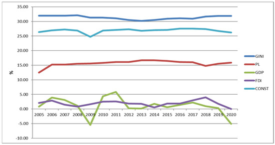
Figure 1.
Denmark. The dynamics of the variables (2005–2020).
FDI dropped sharply in 2008 and 2012 to −10%, and to −5% in 2020, as shown in Figure 1. GINI was resistant to crises and increased gradually. The PL showed a rise (2–3%) in the most difficult years of 2008–2009 and only slightly decreased (1%) in 2020. The GDP was the most sensitive indicator to crises (−5% in 2008–2009, and −5% in 2020). Thus, since most of Denmark’s financial assets were diversified into household balance sheets, the GINI and PL levels did not decline during the crises. CONST was also crisis resilient as long-term investments were involved there. As a result, only external investors reacted to the crises by reducing the flow of FDI. This had a serious impact on the GDP.
3.1.2. Italy
Italy is the fourth largest net contributor within the EU. Italy represents an interesting case study because it has one of the highest rates of the risk of poverty in Europe (Coppola and Di Laurea 2016). By the onset of the financial crisis, COVID-19, Italy was still recovering from the economic fallout from the 2008 financial crisis and the sovereign debt crisis that began more than a decade ago. In addition to the loss of 1.4 million jobs in manufacturing and construction, Italy stagnated (Pinelli et al. 2017). Italy lacked investment in the construction sector. The political culture, which was represented by the pattern of support for political parties at different points on the political spectrum, had a significant impact on FDI (Mudambi and Navarra 2003). Previous structural reforms focused on deregulating labor markets and restructuring the state budget. Since the peak of the sovereign debt crisis in 2012, the Italian economy grew noticeably slower than the economy of the Iberian Peninsula. By 2019, the situation on the Italian labor market had improved only slightly, with an unemployment rate of 9.95% (Eurostat 2020). Since 2012, the unemployment rate in Italy was significantly higher than the EU average, which is 6.4% (Eurostat 2020). At the same time, austerity policies slowed down economic reforms. The forced familialism, unbalanced gender arrangements, territorial cleavages, and sluggish growth rendered Italy vulnerable to financial crisis (Saraceno and Benassi 2020). All these factors affected the dynamics of the GDP, which took negative values during the crises (Figure 2).
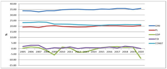
Figure 2.
Italy. The dynamics of variables (2005–2020).
Since the FDI level was only 1–3% of the GDP (Figure 2) and the construction sector accounted for 20–24% of the GDP, this created additional risks in financial crises.
3.1.3. Germany
Germany is one of the most economically prosperous countries in the EU. The causal relationship between FDI and the GDP in Germany is shown in many studies (Cantwell and Bellak 1998; Camarero et al. 2019), as well as the impact of FDI on the labor market and the socioeconomic situation of the population (Arnal and Hijzen 2008). Germany has a vibrant economy and financial system that moves funds to economic agents that have the most productive investment opportunities. The construction sector accounted for 27–28% of the GDP (Figure 3).
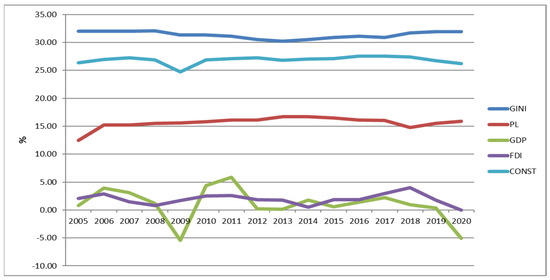
Figure 3.
Germany. The dynamics of variables (2005–2020).
The GINI of Germany was 32–33% in different years, which was close to Italy (35.9%), but worse than Denmark (28.7%). The GDP level reacted strongly to the crises (2008, 2020), losing 5–7 percentage points.
3.1.4. Romania
In recent decades, Romania’s priorities have shifted toward international capital flows as an additional way to finance domestic economic growth. In the period 2005–2016 Romania attracted more FDI and grew bilateral FDI because of the EU membership (Sârbu 2015), Figure 4.
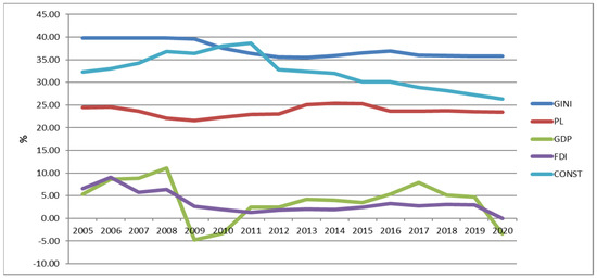
Figure 4.
Romania. The dynamics of variables (2005–2020).
Romania’s FDI share of the GDP was more than that of Denmark, Italy, and Germany (Figure 1, Figure 2 and Figure 3) in percentage terms. However, compared to these countries, Romania had a high GINI ratio and poverty level (PL), which in some years reached 25%. Figure 4 clearly shows how unstable the GDP level was during the 2008 crisis, when the drop in the GDP was 16%. Romania passed the 2014 crisis more safely, without a serious drop in GDP; the economic growth was based on consumption of imported goods, and it was driven by a loose fiscal policy and the credit boom. At the same time, there was a lack of investment in construction. In this situation, the Romanian economy became vulnerable, and during the COVID-19 crisis, as a result, the GDP decreased by 10% in 2020 compared to 2019. Thus, Romania did not have a margin of safety for financial crises.
3.1.5. China
China has a special foreign direct investment policy that has long-term implications not only for China, but for the entire world economy. Since the late 1980s China has adopted an open-door policy and attracted FDI to modernize its economy (Chung and Bruton 2008). The largest companies in the world brought their investments with them in the form of the latest technologies and managerial know-how. Although the FDI share of the GDP decreased (1–2%), it remained high; in 2019 FDI was USD 140 billion, and in 2020 USD 163 billion (Reuters Staff 2021), Figure 5.
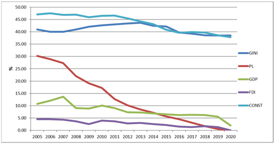
Figure 5.
China. The dynamics of variables (2005–2020).
The construction investments share of the GDP was a record number of 37–45% in different years. The dynamics of poverty reduction (PL, poverty headcount ratio at national poverty lines (% of population)) was unique for the global economy: it dropped from 30.2% in 2005 to 0.04% in 2020.
3.1.6. India
India, like China, is open to FDI, but it is not as susceptible to foreign technology. India has many free trade zones. Because of poor infrastructure, the impact of FDI varied greatly across sectors in regions of India. The research confirmed that the improvement in per capita income, private consumption expenditure, globalization index, and currency value appreciation played a crucial role in increasing FDI inflows into India (Sharma and Kautish 2020). Poverty (PL) was more than halved, from 35% (2005) to 15% (2020), Figure 6. Annual GDP growth was at 7–8%, apart from the crisis years 2008, 2009, 2020.
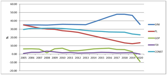
Figure 6.
India. The dynamics of variables (2005–2020).
The construction sector investments in 2005–2020 accounted for a significant share of the GDP at 25–30%. Thus, in a linear relationship, we did not observe a change in poverty based on FDI and investment in construction, but cause-and-effect relationships recorded a change in PL and GDP.
3.1.7. Russian Federation
In 2005–2020 Russia experienced high prices for oil and gas, especially in 2005–2008. The Russian state budget continued to depend on oil and gas revenues, although the share of budget revenues from oil and gas dropped to 40%. Therefore, the Russian government had the opportunity, despite the sanctions from many countries, to support socioeconomic programs and not increase poverty. Unlike China and India, however, Russia did not have a sufficient flow of FDI (1–3% of the GDP) because political and sanctions problems held back foreign investors. According to the Bank of Russia, in 2020 foreign direct investment decreased fourfold, amounting to only USD 8.6 billion. Of this, USD 7.2 billion was foreign investment in Russian investment projects. Over the past 10-year period, the lowest FDI was in 2015. Because of the small FDI inflow, Russia was unable to develop technologies in most industries, which is how it differed from China and India. As a result, the PL decreased only from 18% to 12% for 2005–2020 (Figure 7).
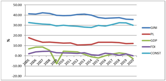
Figure 7.
Russian Federation. The dynamics of variables (2005–2020).
In Russia, large funds were invested in infrastructure, but they were not sufficient for the size of the country. The GINI coefficient was high (≈40%), although it tended to decrease. Thus, in Russia, only a few sectors related to infrastructure and the military industry received state aid, and the GDP dropped sharply during periods of financial crisis.
3.2. Second Stage. The Testing Variables GINI, PL (Dependent); GDP, FDI, CONST, Time (Independent)
Table 2 presents the ARDL model statistics for the dependent variables GINI and PL and the independent variables GDP, FDI, CONST, and the Dickey–Fuller test statistics that correspond to the Engle–Granger cointegration tests. We included annual data for 2005–2020 as well as the time trend in each system. The test statistics suggested that the series were cointegrated at least at the 10% level of significance. Thus, we estimated Equation (1), and Table 2 reports the estimated coefficients for this equation.
If we look at the estimated coefficient, we see that, in different countries, the GINI, PL, and degree of association with the independent variables were different. Thus, for poverty indicators the significance of the GDP was more influential in China (0.38; 0.64) and India (0.72; 0.36). The significance of FDI for poverty alteration was higher in Italy (0.47; 0.42), China (0.28; 0.85), and India (1.5; 0.5). CONST was greater in Denmark (0.43; 0.25), Germany (0.45), India (0.29), and Russia (0.26).
In addition, some coefficients tended to be negative, which means that the situation was unstable and might change for the better or worse. We also observed a different level of significance (p-value, *, **, ***) both in variables and by country. The probability value (p-value) for a given statistical model is the probability that, if the null hypothesis is true, the statistical summary will be greater than or equal to the actual observed results. The data showed that more research is needed for India and China in the future. Perhaps this is because the change in the PL in these countries in 2005–2020 was very significant and poverty was noticeably reduced.
3.3. Third Stage. The Testing Variables PL (Dependent); GDP, FDI, Time (Independent)
Because the change in the PL in some countries was significant, we looked for the relationship between the PL and the GDP, FDI, time. Since we determined the significance of time in testing the time series, we applied a lag (time shift), Table 3.
While examining completely different countries in terms of economic development, we investigated which was more important for poverty reduction: the GDP or FDI? As before, in testing, we corrected heteroscedasticity—the inconstancy of deviations of actual values from the calculated ones, i.e., variability of deviations, and cointegration of time series. The coefficient of determination R2—the proportion of the variance of the dependent variable explained by the considered dependence model—showed high values for all countries (0.99).
We found a strong relationship between an increase in GDP and a decrease in poverty in China (0.46). Considering that the decline in the PL in China was unique in the global economy—30.2% in 2005 and 0.04% in 2020—we concluded that, to reduce poverty, GDP growth cannot be 1–2% per year but must be higher at 5–7% or more. If this GDP growth is maintained for 5 years, then even financial crises such as a global one similar to COVID-19 cannot significantly affect poverty rates, even with negative GDP dynamics. The impact of FDI on the poverty level was accordingly a regression coefficient in Italy (0.18), Romania (0.19), China (0.22), and India (0.29). Thus, test statistics supported the proposition that even when a country has a high GDP, foreign investments have a positive impact on poverty reduction. With foreign investment, countries can reduce poverty even in financial crises.
4. Discussion
Previous studies have examined the impact of investment on poverty in one country or used similarly economically developed countries for comparison. We considered seven countries located on different continents and significantly different in socioeconomic development. We did not present political approaches to attracting foreign investment and did not delve into the social aspects that play a significant role in the investment process; we recorded only the results of changes in the variables (GINI, PL, GDP, FDI, CONST) using linear and time series models (ARDL) and made conclusions.
In our discussion of the results, we recalled that there are several theories of endogenous investment-related growth, as well as theories of inequality and growth. Although the theory of Adam Smith (Smith 2016) is mentioned less in the literature, he was the first to see the dependence of production, labor, land, and capital. As a result, dynamic markets and industrial specialization are winning. The economic development of all countries is different; therefore, Adam Smith’s theory is relevant for developing and transitional countries today. The Harrod–Domar model (Tourette 1964) is used in development economics to explain the growth rate of an economy in terms of savings and capital. For our study, according to the Harrod–Domar model, three types of growth are of interest: the guaranteed growth (the economy does not expand indefinitely and does not fall into recession), the actual growth (real growth of the country’s GDP per year), and the natural growth rate (growth required for the economy to maintain full employment). Consistent with Thomas Malthus’s theory (Hollander 1997), cross-country analysis reveals a significant positive effect of technological level on population density and a negligible effect on per capita income over 1–1500 years. The Solow–Swan theory (Solow 2001) proposes that the return on capital and labor declines over time. Capital accumulates through investments, but its level or stock is constantly decreasing due to depreciation. Further, within the framework of our small study, we concentrated on only some provisions of the theories and models of endogenous growth to reduce poverty in each of the countries under consideration.
According to the results of Section 3.1, in Denmark, financial crises (2008, 2014, and 2020) practically did not affect the GINI and PL, since high household assets, although accompanied by a high level of household debt, kept the poverty level low. We found confirmation of this conclusion in the ARDL model (Table 2 and Table 3). Low values of the variable coefficients GDP (0.05–0.08) and FDI (0.0007–0.04) confirmed the value of the Harrod–Domar model.
Italy is the country where Adam Smith’s theory is fully implemented to this day. Our data showed that since 2005 the PL did not change and was about 20%, and the GINI coefficient added two percentage points from 2005 to 2020 and was 35.8%. The regression coefficient in the ARDL model, the dependence of the PL on FDI, was 0.18–0.47. Thus, labor production and capital were closely related, investment in construction and external investment were small, so all financial crises seriously affected the Italian economy.
In Germany, the ARDL model variables showed only a significant relationship between investment in construction (CONST) and PL (coefficient 0.42). The causal relationship between GINI and PL on account of FDI and GDP was weak. Germany combines several models of economic growth. However, in the example of Germany, it can be seen that Malthus’s theory, a significant positive effect of the technological level on population density and a negligible effect on per capita income, were confirmed with our calculations since the GDP reacted sharply to all financial crises while the levels of GINI and PL were maintained in Germany.
In Romania, compared with other countries, in 2005–2020 PL fluctuations were the greatest; that is, poverty either increased or decreased (+/−4%). The dynamics of the GDP (−15%) during financial crises showed significant volatility. Romania was open to foreign investment and in 2006 the FDI accounted for 9% of the GDP. But in Romania, capital accumulated through investment, and its level and stock constantly decreased due to depreciation; therefore, there was strong volatility in the GDP and PL. In any case, we confirmed the Solow–Swan theory in Romania.
China has adopted an open-door policy and attracted FDI to modernize its economy. Additionally, in 2005–2020 China’s PL was unique in the global economy: it dropped from 30.2% in 2005 to 0.04% in 2020; GINI dropped from 45 to 38% (2005–2020). China has attracted not only foreign investments but also foreign technologies at the same time. Therefore, the GDP dynamics showed the highest results among all countries: in 2007 it was +13%, in 2010 +10%, in 2019 +5.5%, and in 2020 −1.9%. We concluded that China combined the most famous theories of economic growth (the Adam Smith theory, the Harrod–Domar model, the Malthusian theory and Solow and Swan’s model) linking investment, productive labor, accumulation, and technology. As a result, all the models were present in China (2005–2020) and the country quickly coped with the pandemic and steadily experienced the 2020 financial crisis. Our calculations from the ARDL model confirmed this: the dependence of the PL on the GDP was the coefficient 0.38–0.54, the FDI was 0.2–0.8.
In India, poverty was more than halved from 2005 (PL 35%) to 2020 (PL 15%). Annual GDP growth was at the level of 7–8%, apart from the crisis years 2008, 2009, 2020. The correlation coefficient of the ARDL model showed a close relationship of GINI (0.76) and PL (0.32) with the GDP; and of GINI (1.5) and PL (0.5) with FDI. We confirmed the Harrod–Domar model in India, where capital accumulation and savings were not enough for financial resilience in crises. Therefore, for India, attracting foreign investment will be positive. We also found evidence of the working theory of Adam Smith since the return on investment was closely related to the location of production and less investment went to poor areas. In the coming years, India needs to further increase the flow of foreign investment, given the fact that their profitability will gradually decline.
In the Russian Federation, our testing showed a slight dependence of the GINI coefficient on GDP—0.18. The dependence of the poverty level (PL) on the GDP and FDI was weak, from 0.03 to 0.013. The correlation dependence was traced between the poverty level (PL) and investment in construction (CONST)—0.26. The GINI coefficient was high (≈40%), and the PL decreased from 18 to 12% for 2005–2020, although oil and gas revenues provided the economy with large financial revenues in the state budget. Despite the income, an economic development took place in only a few related sectors (the military—industrial complex and the infrastructure). Foreign investment was scarce, and most of it came from offshore companies. In the Russian Federation, we did not find that the previously listed theories of endogenous growth were implemented. Adam Smith’s theory was not sufficiently implemented in the parameters of land–capital. The Harrod–Domar model lacked guaranteed growth. The return on capital decreased (Solow–Swan) and the technological level did not reduce poverty (Malthus’s theory). Financial crises, when the GDP falls to 7–10%, are survived only through financing from the state stabilization funds. In the Russian Federation, there is no holistic theory of economic growth.
5. Conclusions
The main purpose of this study is to investigate empirically the direct impact of GDP, FDI and investment in construction on poverty and compare the Russian Federation with some developed and developing countries. We carried out the research in three stages: 1. An assessment of the dynamics of the variables over 2005–2020 and the factor countries (Denmark, Italy, Germany, Romania, China, India, the Russian Federation); 2. Testing variables: GINI, PL—dependent; GDP, FDI, CONST, time—independent; 3. Testing variables: PL—dependent; GDP, FDI, time—independent. Based on the theoretical discussions, and empirical experiences, and the use of statistics from seven countries the period of 2005–2020, the following conclusions can be drawn.
We found a strong relationship between an increase in GDP and a decrease in poverty. We concluded that to reduce poverty, GDP growth cannot be 1–2% per year but must be higher at 5–7% or more. If this GDP growth is maintained for 5 years, then even financial crises such as a global one similar to COVID-19 cannot significantly affect poverty rates, even with negative GDP dynamics. Test statistics supported the proposition that when a country has a high GDP, foreign investments have a positive impact on poverty reduction. With foreign investment, countries can reduce poverty even in financial crises.
Using several theories of economic development in our analysis, we came to the conclusion that the “Chinese economic miracle” that we see in the form of poverty reduction from 30.2% in 2005 to 0.04% in 2020; GINI dropped from 45 to 38% (2005–2020), consists not only of technology or investment. China effectively uses the theories of endogenous economic growth, putting scientific knowledge into practice. The government of the Russian Federation has been making only isolated actions to stabilize the economy in the past 15 years, which cannot significantly support economic development. In the Russian Federation, there is no holistic theory of economic growth. Therefore, poverty will grow during crises. We intend to continue our research in this area. We recommend expanding the number of independent variables and increasing the number of countries, since comparing economically different countries reveals more factors in the changes in poverty levels.
Author Contributions
Conceptualization, methodology, writing, T.S.; investigation, E.S.; resources, N.F.; supervision and writing, N.K.; funding acquisition, Y.K. All authors have read and agreed to the published version of the manuscript.
Funding
This research received no external funding.
Institutional Review Board Statement
Informed consent was obtained from all subjects involved in the study.
Informed Consent Statement
Informed consent was obtained from all subjects involved in the study.
Data Availability Statement
Databank of the World Bank: https://databank.worldbank.org/home.aspx (accessed on 15 August 2021). The People’s Bank of China: http://www.pbc.gov.cn/en/3688006/index.html (accessed on 15 August 2021). The Central Bank of India: https://www.centralbankofindia.co.in/en (accessed on 15 August 2021). The Eurostat Database: https://ec.europa.eu/eurostat/data/database (accessed on 15 August 2021). The Bank of Russia: The Bank of Russia.
Conflicts of Interest
The authors declare no conflict of interest.
References
- Adato, Michelle, Michael R. Carter, and Julian May. 2006. Exploring poverty traps and social exclusion in South Africa using qualitative and quantitative data. The Journal of Development Studies 42: 226–47. [Google Scholar] [CrossRef] [Green Version]
- Ahmad, Munir, Zhen-Yu Zhao, Muhammad Irfan, and Marie Claire Mukeshimana. 2019. Empirics on influencing mechanisms among energy, finance, trade, environment, and economic growth: A heterogeneous dynamic panel data analysis of China. Environmental Science and Pollution Research 26: 14148–14170. [Google Scholar] [CrossRef] [PubMed]
- Akaike, Hirotugu. 1981. This Week’s Citation Classic. Current Contents Engineering, Technology, and Applied Sciences 12: 42. Available online: http://www.garfield.library.upenn.edu/classics1981/A1981MS54100001.pdf (accessed on 28 September 2021).
- Anand, Abhishek. 2019. FDI and Its Role in Developing Economy. 4. Available online: https://rrjournals.com/wp-content/uploads/2020/09/2102-2104_RRIJM190404444.pdf (accessed on 28 September 2021).
- Andersen, Torben M. 2015. A flexicurity labor market during recession. IZA World of Labor 173. [Google Scholar] [CrossRef] [Green Version]
- Anetor, Friday Osemenshan. 2019. Economic growth effect of private capital inflows: A structural VAR approach for Nigeria. Journal of Economics and Development 21: 18–29. [Google Scholar] [CrossRef] [Green Version]
- Antoniades, Andreas, Indra Widiarto, and Alexander S. Antonarakis. 2020. Financial Crises and the Attainment of the SDGs: An Adjusted Multidimensional Poverty Approach. Sustainability Science 15: 1683–98. [Google Scholar] [CrossRef] [Green Version]
- Arnal, Elena, and Alexander Hijzen. 2008. The Impact of Foreign Direct Investment on Wages and Working Conditions. Available online: https://scholar.google.com/scholar?hl=en&as_sdt=0%2C5&q=Arnal%2C+E.%2C+and+A.+Hijzen.+%E2%80%98The+Impact+of+Foreign+Direct+Investment+on+Wages+and+Working+Conditions%E2%80%99%2C+2008.&btnG= (accessed on 28 September 2021).
- Asian Development Bank. 2021. Asian Development Bank and India: Fact Sheet (India). Available online: https://www.adb.org/sites/default/files/publication/27768/ind-2020.pdf (accessed on 28 September 2021).
- Azam, Muhammad, and Yi Feng. 2021. Does Foreign Aid Stimulate Economic Growth in Developing Countries? Further Evidence in Both Aggregate and Disaggregated Samples. Quality & Quantity, 1–24. [Google Scholar] [CrossRef]
- Ball, Michael, and Andrew Wood. 1996. Does building investment affect economic growth? Journal of Property Research 13: 99–114. [Google Scholar] [CrossRef]
- Bebczuk, Ricardo. 2003. Asymmetric Information in Financial Markets Cambridge Books. Cambridge Books. Cambridge: Cambridge University, Available online: https://ideas.repec.org/b/cup/cbooks/9780521797320.html (accessed on 28 September 2021).
- Bermejo Carbonell, Jorge, and Richard A. Werner. 2018. Does Foreign Direct Investment Generate Economic Growth? A New Empirical Approach Applied to Spain. Economic Geography 94: 425–56. [Google Scholar] [CrossRef]
- Bhuimali, Anil, Partha Pratim Sengupta, Sidhartha Sankar Laha, and Madhabendra Sinha. 2019. FDI, Trade, and Economic Growth: A Dynamic Panel Study on Global Economy. In The Gains and Pains of Financial Integration and Trade Liberalization. Edited by Rajib Bhattacharyya. Bingley: Emerald Publishing Limited, pp. 77–87. [Google Scholar] [CrossRef]
- Camarero, Mariam, Laura Montolio, and Cecilio Tamarit. 2019. What Drives German Foreign Direct Investment? New Evidence Using Bayesian Statistical Techniques. Economic Modelling 83: 326–45. [Google Scholar] [CrossRef]
- Cantwell, John, and Christian Bellak. 1998. How Important Is Foreign Direct Investment? Oxford Bulletin of Economics and Statistics 60: 99–106. [Google Scholar] [CrossRef]
- Chung, Ming Lau, and Garry D. Bruton. 2008. FDI in China: What We Know and What We Need to Study Next. Academy of Management Perspectives 22: 30–44. [Google Scholar] [CrossRef]
- Coppola, Lusia, and Davide Di Laurea. 2016. Dynamics of Persistent Poverty in Italy at the Beginning of the Crisis. Genus 72: 1–17. Available online: https://genus.springeropen.com/articles/10.1186/s41118-016-0007-x (accessed on 28 September 2021). [CrossRef] [Green Version]
- Coulibaly, Sara Elder, Phu Huynh, Arun Kumar, Dong Eung Lee, Bashar Marafie, Yuki Otsuji, and Netsanet Tesfay. 2021. COVID-19 and Multinational Enterprises: Impacts on FDI, Trade and Decent Work in Asia and the Pacific. ILO Brief. Available online: https://www.researchgate.net/profile/Pelin-Sekerler-Richiardi/publication/350994880_COVID-19_and_multinational_enterprises_Impacts_on_FDI_trade_and_decent_work_in_Asia_and_the_Pacific/links/607e97ad2fb9097c0cf7632e/COVID-19-and-multinational-enterprises-Impacts-on-FDI-trade-and-decent-work-in-Asia-and-the-Pacific.pdf (accessed on 28 September 2021).
- Dhrifi, Abdelhafidh, Raouf Jaziri, and Saleh Alnahdi. 2020. Does Foreign Direct Investment and Environmental Degradation Matter for Poverty? Evidence from Developing Countries. Structural Change and Economic Dynamics 52: 13–21. [Google Scholar] [CrossRef]
- Dickey, David A., and Wayne A. Fuller. 1981. Likelihood ratio statistics for autoregressive time series with a unit root. Econometrica 49: 1057–72. [Google Scholar] [CrossRef]
- Drabek, Zdenek. 2021. Governance of FDI and the East Asian Economic Community. Asia and the Global Economy 1: 100001. [Google Scholar] [CrossRef]
- Durbin, James, and Geoffrey Watson. 1950. Testing for Serial Correlation in Least Squares Regression: I. Biometrika 37: 409–28. [Google Scholar] [CrossRef]
- Engle, Robert F., and Clive W. J. Granger. 1987. Co-Integration and Error Correction: Representation, Estimation, and Testing. Econometrica 55: 251–76. [Google Scholar] [CrossRef]
- Eurostat. 2020. Europe 2020 Indicators—Poverty and Social Exclusion. Available online: https://ec.europa.eu/eurostat/statistics-explained/index.php?title=Archive:Europe_2020_indicators_-_poverty_and_social_exclusion&oldid=394836 (accessed on 28 September 2021).
- Fang, Jing, Alan Collins, and Shujie Yao. 2021. On the Global COVID-19 Pandemic and China’s FDI. Journal of Asian Economics 74: 101300. [Google Scholar] [CrossRef]
- Friedman, Milton, and Anna J. Schwartz. 1991. A Monetary History of the United States 1867–1960 (1963). The American Economic Review 81: 1. Available online: www.jstor.org/stable/2006787 (accessed on 28 September 2021).
- Hillebrandt, Patricia M. 2000. Economic Theory and the Construction Industry. London: Palgrave Macmillan UK, p. 224. [Google Scholar] [CrossRef]
- Hollander, Samuel. 1997. The Economics of Thomas Robert Malthus. Toronto: University of Toronto Press, vol. 4. [Google Scholar] [CrossRef]
- Jensen, Per H. 2017. Danish Flexicurity: Preconditions and Future Prospects. Industrial Relations Journal 48: 218–30. [Google Scholar] [CrossRef]
- Jensen, Thais Lærkholm, and Niels Johannesen. 2017. The Consumption Effects of the 2007–2008 Financial Crisis: Evidence from Households in Denmark. American Economic Review 107: 3386–414. [Google Scholar] [CrossRef] [Green Version]
- Kargi, Bilal. 2013. Integration between the Economic Growth and the Construction Industry: A Time Series Analysis on Turkey (2000–2012). Political Economy—Development: Public Service Delivery EJournal 2013: 20–34. [Google Scholar] [CrossRef] [Green Version]
- Kastratović, Radovan. 2020. The Impact of Foreign Direct Investment on Host Country Exports: A Meta-Analysis. The World Economy 43: 3142–83. [Google Scholar] [CrossRef]
- Knoerich, Jan. 2017. How Does Outward Foreign Direct Investment Contribute to Economic Development in Less Advanced Home Countries? Oxford Development Studies 45: 443–59. [Google Scholar] [CrossRef]
- Krygina, A. M., I. P. Avilova, M. I. Oberemok, and A. G. Grebenik. 1088. Modeling of Organizational and Functional Components of Investment and Construction Controlling in the Reproduction of Eco-Residential Real Estate. Bristol: IOP Publishing. [Google Scholar] [CrossRef]
- Ly, Bora. 2021. The Implication of FDI in the Construction Industry in Cambodia under BRI. Edited by Albert Tan. Cogent Business & Management 8: 1875542. [Google Scholar] [CrossRef]
- Ma, Le, Chunlu Liu, and Richard Reed. 2017. The Impacts of Residential Construction and Property Prices on Residential Construction Outputs: An Inter-Market Equilibrium Approach. International Journal of Strategic Property Management 21: 296–306. [Google Scholar] [CrossRef]
- Mahembe, Edmore, and Nicholas Odhiambo. 2019. Foreign Aid, Poverty and Economic Growth in Developing Countries: A Dynamic Panel Data Causality Analysis. Cogent Economics & Finance 7: 1626321. [Google Scholar] [CrossRef]
- Mainassara, Yacouba Boubacar, and Célestin C. Kokonendji. 2016. Modified Schwarz and Hannan–Quinn Information Criteria for Weak VARMA Models. Statistical Inference for Stochastic Processes 19: 199–217. [Google Scholar] [CrossRef]
- Mamun, Muhammed, and Irfan Ullah. 2020. COVID-19 Suicides in Pakistan, Dying off Not COVID-19 Fear but Poverty?–The Forthcoming Economic Challenges for a Developing Country. Brain, Behavior, and Immunity 87: 163. [Google Scholar] [CrossRef]
- Mehar, Muhammad Ayub Khan. 2021. Bridge financing during covid-19 pandemics: Nexus of FDI, external borrowing and fiscal policy. Transnational Corporations Review 13: 109–24. [Google Scholar] [CrossRef]
- Michael Osterwald-Lenum Statistics. 2017. Household Balance Sheet Structure in Denmark and Sensitivity to Rising Rates. Available online: https://www.elibrary.imf.org/view/journals/002/2017/159/article-A001-en.xml (accessed on 28 September 2021).
- Mishkin, Frederic S. 1992. Anatomy of a Financial Crisis. Journal of Evolutionary Economics 2: 115–30. [Google Scholar] [CrossRef] [Green Version]
- Mudambi, Ram, and Pietro Navarra. 2003. Political Culture and Foreign Direct Investment: The Case of Italy. Economics of Governance 4: 37–56. [Google Scholar] [CrossRef]
- Pesaran, M. Hashem, Yongcheol Shin, and Richard J. Smith. 2001. Bounds testing approaches to the analysis of level relationships. Journal of Applied Econometrics 16: 289–326. [Google Scholar] [CrossRef]
- Pinelli, Dino, Roberta Torre, Lucianajulia Pace, Laura Cassio, and Alfonso Arpaia. 2017. The Recent Reform of the Labour Market in Italy: A Review. European Economy Discussion Papers. Available online: https://ec.europa.eu/info/sites/default/files/economy-finance/dp072_en.pdf (accessed on 28 September 2021).
- Ranaldo, Angelo, and Fabricius Somogyi. 2021. Asymmetric Information Risk in FX Markets. Journal of Financial Economics 140: 391–411. [Google Scholar] [CrossRef]
- Reuters Staff. 2021. China Was Largest Recipient of FDI in 2020: Report, REUTERS Edition ed. January 25. Available online: https://www.reuters.com/article/us-china-economy-fdi-idUSKBN29T0TC (accessed on 28 September 2021).
- Ripamonti, Alexandre. 2020. Financial Institutions, Asymmetric Information and Capital Structure Adjustments. The Quarterly Review of Economics and Finance 77: 75–83. [Google Scholar] [CrossRef]
- Ruddock, Les, and Jorge Lopes. 2006. The Construction Sector and Economic Development: The “Bon Curve”. Construction Management and Economics 24: 717–23. [Google Scholar] [CrossRef]
- Saraceno, Chiara, and David Benassi. 2020. Poverty in Italy: Features and Drivers in a European Perspective. Bristol: Policy Press, ISBN 978-1447352211. [Google Scholar]
- Sârbu, Maria-Ramona. 2015. The Impact of Foreign Direct Investment on Economic Growth: The Case of Romania. Acta Universitatis Danubius: Oeconomica 11: 4. Available online: http://journals.univ-danubius.ro/index.php/oeconomica/article/view/2820/2839 (accessed on 28 September 2021).
- Sharma, Rajesh, and Pradeep Kautish. 2020. Examining the Nonlinear Impact of Selected Macroeconomic Determinants on FDI Inflows in India. Journal of Asia Business Studies. [Google Scholar] [CrossRef]
- Shin, Yongcheol, Byungchul Yu, and Matthew Greenwood-Nimmo. 2014. Modelling asymmetric cointegration and dynamic multipliers in a nonlinear ARDL framework. In Festschrift in honor of Peter Schmidt. New York: Springer, pp. 281–314. [Google Scholar] [CrossRef]
- Shukur, Ghazi, and Panagiotis Mantalos. 2000. A Simple Investigation of the Granger-Causality Test in Integrated-Cointegrated VAR Systems. Journal of Applied Statistics 27: 1021–31. [Google Scholar] [CrossRef]
- Simplice, Asongu, and Nicholas M. Odhiambo. 2020. Foreign Direct Investment, Information Technology and Economic Growth Dynamics in Sub-Saharan Africa. Telecommunications Policy 44: 101838. [Google Scholar] [CrossRef]
- Smith, Adam. 2016. The Wealth of Nations. Aegitas. Available online: https://books.google.ru/books/about/The_Wealth_of_Nations.html?id=lMgDDQAAQBAJ&redir_esc=y (accessed on 28 September 2021).
- Solow, Robert. 2001. From Neoclassical Growth Theory to New Classical Macroeconomics. In Advances in Macroeconomic Theory. Berlin/Heidelberg: Springer, pp. 19–29. [Google Scholar] [CrossRef]
- Toda, Hiro Y., and Taku Yamamoto. 1995. Statistical Inference in Vector Autoregressions with Possibly Integrated Processes. Journal of Econometrics 66: 225–50. [Google Scholar] [CrossRef]
- Tourette, John E. La. 1964. Technological Change and Equilibrium Growth in the Harrod-domar Model. Kyklos 17: 207–26. [Google Scholar] [CrossRef]
- Watanabe, Sumio. 2013. A Widely Applicable Bayesian Information Criterion. Journal of Machine Learning Research 14: 867–97. Available online: https://www.jmlr.org/papers/volume14/watanabe13a/watanabe13a.pdf (accessed on 28 September 2021).
- Zhang, Xiaobo, and Kevin H. Zhang. 2003. How Does Globalisation Affect Regional Inequality within A Developing Country? Evidence from China. The Journal of Development Studies 39: 47–67. [Google Scholar] [CrossRef]
Publisher’s Note: MDPI stays neutral with regard to jurisdictional claims in published maps and institutional affiliations. |
© 2021 by the authors. Licensee MDPI, Basel, Switzerland. This article is an open access article distributed under the terms and conditions of the Creative Commons Attribution (CC BY) license (https://creativecommons.org/licenses/by/4.0/).