1. Introduction
The South-East Asia financial crisis of the late twentieth century was an unexpected (
Krugman 1999) development that saw a rapid deterioration of the economies (
Suryahadi et al. 2012) and financial markets (
Choudhry et al. 2007;
Click and Plummer 2005;
Khan et al. 2009) of several South-East Asian countries. Several of the countries directly impacted by the crisis had experienced significant economic growth in the years previous to the crisis (
Huang and Xu 1999). There were several major events during the crisis, such as Thailand floating the currency as well as political changes such as the high profile replacement in Malaysia of the finance minister, creating a very complex economic and financial situation. External factors, such as the IMF intervention, have been also frequently cited as detrimental (
Bello 1999) further adding complexity to the crisis with some authors, such as
Pilbeam (
2001), suggesting that some of the programs introduced by the IMF were too harsh. In fact,
Miller (
1998) considers that it is more precise describing the situation as multiple crisis occurring simultaneously rather than a single crisis.
Akyuz (
1998) mentioned the substantial differences in the economies of the countries involved in the crisis. Some of the countries/regions more heavily impacted by this crisis were Thailand, where the crisis arguably started, Malaysia, Indonesia, South Korea, and the Philippines.Some authors, such as
Dickinson and Mullineux (
2001), have mentioned that one major factor behind the crisis was the ineffective financial regulation in some of the countries impacted. Singapore and Hong Kong were also involved in the financial crisis but they were significantly less impacted (
Jin 2000), arguably due to a combination of stronger (pre-crisis) financial oversight and regulations as well as relatively high foreign exchange reserves. To put it into context, the Singaporean economy contracted in 1998 only 2.2%. Of the countries directly involved in the South-East Asia financial crisis, only the Philippines experienced a smaller contraction in 1998. Indonesia for instance had a GDP contraction in 1998 of 13.1%. Authors such as
Tee (
2003) mentioned that the credibility of the Singaporean dollar exchange rate and the sound economic situation of Singapore before the South-East Asia financial crisis were among the major factors protecting the currency during this period; nevertheless, Singapore was clearly also impacted. The capital markets as well as the currencies of most of the above mentioned countries and jurisdictions were impacted to various degrees (
Goldstein 1998). Notably, not all the Asian currency pegs were broken during the crisis with for instance Hong Kong managing to successfully defend the Hong Kong dollar from multiple speculative assaults. One factor facilitating maintaining the peg was the large reserves of foreign capital held by Hong Kong, second only in the region of those of Mainland China (
Chirathivat 2007). Hong Kong strongly defended the currency peg with the Monetary Authority of Hong Kong, the de facto central bank of Hong Kong, using its reserves to support the Hong Kong dollar. For instance, it was reported that the HKMA spent in two hours on 24 July 1997 one billion U.S. dollars supporting the Hong Kong dollar (
Kearney and Hutson 1999). Some authors, such as
Bennett (
1994), have mentioned the importance of the different types of peg.
Bennett (
1994) compares the case of Hong Kong with a hard peg and Singapore with adjustable peg.
While Hong Kong overcame the South-East Asia financial crisis better than most of its regional neighbours and was able to maintain the peg with the U.S dollar, it was also clearly affected by the crisis. According to data from the IMF, the Hong Kong economy managed to grow in 1997, with GDP up 5.1%, but contracting in 1998 by approximately 5.5%. Economic growth remained positive in the following years. The performance of the Hong Kong economy during this period considerably lagged that of Mainland China. Remarkably, Mainland China did not have during this period a single year of negative growth with GDP increasing 9.3% and 7.8% in 1997 and 1998, respectively. GDP growth in the post-crisis period in Hong Kong remained positive but volatile with oscillations such as a GDP increase of 10.0% in 2000 followed by a GDP increase of only 0.6% in 2001. The stock market in Hong Kong was also impacted by the crisis with the Hang Seng Index down approximately 46% from the peak in 7 August 1997 of 16,673 to the bottom of 28 October 1997 of 9059.
The 1997 South-East Asia financial crisis brought to an abrupt stop (
Miller (
1998)) the remarkable rates of economic growth experienced by several of the countries in the region. Some authors, such as
Corsetti et al. (
1999), suggest that the South-East Asia financial crisis of 1997–1998 was the culmination of a series of long standing pre-existing structural imbalances rather than a single major event precipitating the crisis but this remains an area of debate. The degree of development and sizes of these economies involved were remarkably different. As previously mentioned, one of the most visible and first events during this financial crisis was the collapse of the Thai currency (baht) adding pressure on Thai companies that have borrowed on U.S. dollars. This is in fact the start of the crisis according to authors such as
Leightner (
2007). The situation in Thailand rapidly spread to other countries (
Jomo 1998).
Most of the existing literature in the South-East Asia financial crisis focuses on the impact on the real economy as well as in the fluctuations in the foreign exchange market (
Woo et al. 2000). This is perhaps due to some very high profile developments in the foreign exchange market such as the well-known bet of George Soros against the baht. There are also some interesting research, such as
Beaverstock and Doel (
2001), mentioning the role played by the baking sector, of both domestic institutions as well as of the international investment banks.
There is however relatively less literature covering the impact on the stock market, particularly from a short-term event driven angle. Short-term fluctuations in the equity market might have a very substantial impact on investors, particularly if their investments are leveraged or it they are forced to unwind their trades due to margin calls or risk management considerations. Unwinding these positions, during unfavorable market movements, might negate the benefits of a future recovery in the market. There is ample literature suggesting that there are volatility clusters in several equity markets (
Cont 2007;
Lux and Marchesi 2000) and such clusters might potentially be related to a major event. An example of such an event could be Thailand letting its currency to free float during the South-East Asia financial crisis on 2 July 1997. Until that moment, most South-East Asian countries have defended their currencies, many of them pegged to the U.S. dollar. A related factor frequently mentioned in the existing literature (
Radelet and Sachs 1998) is the spread of financial panic. In this paper, we carry out a short-term event driven Granger causality analysis using some important events cited in the existing literature. Granger causality tests are a frequently used technique to analyze dependencies between financial variables (
Ibrahim 2000). The analysis focuses on the impact on the equity markets rather than the impact on the foreign exchange market.
One of the assumptions underlying this paper is that some events, such as, for instance, the end of a currency peg, can trigger significant movements in the local equity market. Furthermore, the impact on those events can also spread to other markets, particularly regional, also impacting their performance. It seems also reasonable to assume that in principle this market fluctuations can be short lived, averaging out over long periods of time, but having substantial impact in the short term. In order to analyze these events, it is necessary to have the appropriate mathematical and statistical tools. Note that the focus on this paper is on trying to determine the changes in interdepenedencies of stock markets rather that on trying to forecast the stock prices themsleves. In recent years, there has been a focus on using machine learning techniques generating interesting results, such as, for instance, neural networks (
Cervello and Guijarro 2020;
Garcia et al. 2018). However, the analysis in this paper focus on changes in the dynamics of the market with actual forecasting outside of the scope. An underlying assumption in this analysis is that the Granger causality test can detect some causality relationships. This is a common assumption in multiple articles such as
Hoffmann et al. (
2005);
Akinboade and Braimoh (
2010), and
Lopez and Weber (
2017). It is not assumed that the Granger causality test fully accurately reflects underlying causality relationships, but it is rather used as a quantitative indication of their existence. In other words, the Granger causality test reflects Granger causality rather than true underlying causality. Nevertheless, it is important to have a quantitative test that can be applied objectively to the data to try to minimize as much as possible the potential for biases in the analysis.
2. Some Major Events during the South-East Asia Financial Crisis
It is a challenging task to identify the major events during any financial crisis and the South-East Asia financial crisis is no exception and even more complex to determine the factors that might impact the equity market. For instance, besides objective financial conditions there is some existing research on the impact of investors sentiment (
Guijarro et al. 2019) on the equity market. This could be a particularly important factor to be taken into consideration during financial crisis. It is also acknowledged that there is some degree of subjectivity and that there are some other events that could potentially be considered. Nevertheless, it is necessary when attempting to carry out an event driven analysis, to identify a list of such events that are significant enough to have had a large impact on the stock market. In this case of the South-East Asia financial crisis, seven events (
Table 1) were identified as substantial enough to potentially having the capacity to impact the stock market. These events range from 2 July 1997 (
Jansen 2001) that saw the end of the Thai baht peg (event 1) to 3 September 1998 with the replacement of the finance minister in Malaysia (event 7). Some authors such as
Jansen (
2001) consider that the start of the South-East Asia financial crisis was July 1997, coinciding with the end of the Thai baht peg.
Krongkaew (
1999), more explicitly, mentions that the start of the economic crisis occurs in Thailand with the flotation of its currency. Thus, this event should be one of those analyzed.
Pressure had been building on the Thai economy since early 1997 and was becoming evident with the default of Somprasong Land (
Lauridsen 1998;
Wong 2001), a property developer, adding concerns about the health of property developers. However, this event by itself did not appear to have caused an impact on the broad financial market or economy. Another factor to take into account was the increasing pressure from hedge funds
Robins (
2000) on the baht. Perhaps some of the best known hedge funds to bet against the baht during this period are the Quantum Fund and Tiger Fund with a reportedly one and three billion U.S. dollars short positions on the currency, respectively. Note that the actual impact that the hedge funds had on the South-East Asia financial crisis remains a disputed topic with authors such as
Brown et al. (
2000) not founding empirical evidence that hedge funds caused the financial crisis in Thailand. Regardless of the actual impact of hedge funds, the situation in the currency front eventually became unsustainable and Thailand had to float its currency. After the flotation of the Thai baht there was an almost immediate overnight depreciation compared to the U.S. dollar (
Punyaratabandhu 1998) putting substantial pressure on Thai companies that had borrowed in U.S. dollar terms. The deterioration in returns combined with large amounts of borrowings in foreign currency plus a significant devaluation of the baht proved to be a combination that hurt a large amount of Thai companies that were unable to repay their borrowings.
Jansen (
2001) and several other scholars have mentioned that financial institutions as well as companies got used to have a stable currency pegged to the U.S. dollar creating a false sense of security and causing poor risk management. According to these authors, the possibility of a sudden change in the exchange rate of the baht was regarded as a rather remote possibility and this perception was based on many years of stable foreign exchange values and growing economy. While there were financial tools for hedging currency exposure the borrowing from Thai domestic companies was predominantly not hedged (
Takayasu 1998) and thus companies had to absorb loan repayments denominated in U.S. dollar while the local currency was rapidly depreciating.
Another event considered (event 2) was Indonesia letting its currency to free float in 14 August 1997 (
Pratomo and Warokka 2013). This was arguably unavoidable after Thailand ended its peg a few weeks earlier with the Indonesian currency reserves coming under increasing pressure during those weeks. In the initial stages of the financial crisis Indonesia showed some signs of resilience. This situation quickly changed with the local currency slumping and a run on the banking sector putting the national finances under considerable stress. One of the first clear signs of stress in Indonesian economy appeared in the currency market with the Indonesian rupiah slumping against the U.S. dollar from July 1997 to January 1998. Indonesia had started a process of liberalizing the exchange rate system (
James 2005) in the previous decades and by 1997 the Indonesia rupiah traded within a relatively narrow band relatively to the U.S. dollar. Given the increasing pressure on the currency and the cost of defending it, Indonesia decided on 14 August 1997 to float the currency. The regime shift added significant amount of volatility to the exchange rate and increased economic pressure. Some authors, such as, for instance,
Pratomo and Warokka (
2013), have argued that the Indonesian rupiah was not a stable currency even before the South-East Asia financial crisis and that if more efforts were have done to stabilize it in the years before the crisis the rupiah should have hold substantially better during the crisis period.
After a turbulent summer of 1997, several of the countries engulfed in the crisis developed economic plans to tackle the crisis, such as for instance the restructuring package introduced by the Thai government in 14 October 1997 (event 3). This restructuring initiative received the praise of the IMF with IMF managing director, Mr. Michel Camdemssus, stating “The Thai government has made a significant announcement today about its detailed strategy to restructure Thailand’s troubled financial sector.” An important development of this initiative was the creation in Thailand of the Financial Sector Restructuring Authority commonly known as FRA (
Hawkins 1997). FRA was one of the main agencies in charge of assessing the economic situation and handling troubled financial assets and had a wide range of powers including the ability to request troubled financial companies to recapitalize or to arrange acquisitions by third parties.
An event that attracted substantial attention during the South-East Asia financial crisis was the collapse or Peregrine Investments in early 1998 (event 4). Peregrine Investments went into liquidation in January 1998 in Hong Kong. At the core of the collapse of Peregrine Investments was a 269 million U.S. dollar loan to a taxi company in Indonesia called PT Steady Safe. Several attempts to restructure the loan were unsuccessful with the company going into liquidation relatively quickly after the start of the South-East Asia financial crisis. Note that Peregrine Investments was a very well-regarded institution with diversified operations across Asia and to a lesser degree in Europe and the US. At the time of its collapse it was one of the largest independent investment bank in Asia. A few months later, in 1998, there was a subtle but important development with Thailand modifying the definition of non-performing bank loans (event 5). The objective of this measure was to make the definition of non-performing bank loans in Thailand in line with the international accepted guidelines (
Takayasu 1998). While a positive development, this reclassification arguably added in the short term more pressure on the market as international standards at the time were more stringent.
Another event considered was the successful presidential campaign of Mr. Joseph Estrada in the Philippines (
Claudio 2014;
Ringuet and Estrada 2003), representing the political party PMP, becoming president after winning the elections in 11 May 1998 (event 6). Estrada won the election with a populist message (
Hedman 2001), promising alleviating poverty. The Philippines was one of the very few Asian countries, at the time of the South-East Asia financial crisis to have a fund deposit insurance scheme (
Kochhar et al. 1998), likely helping alleviating runs in the Philippines banks. Additionally the banking sector in the Philippines was less exposed to the real estate sector (
Table 2) that most of its regional peers. This is not to say that the banking system of the Philippines had no significant exposure to the real estate sector. According to
Bello (
1999), the commercial bank loan exposure of the Philippines to the real estate sector was approximately 20% in the period just before the financial crisis, while the real estate exposure in Indonesia during the same period was approximately 25% (
Bello 1999). Several authors, such as
Krugman (
1999), have mentioned that a major issue was that a large amount of the capital borrowed overseas was directed towards investment in real estates. In many occasions, foreign capital was cheaper than domestic one and companies borrowed in foreign currency increasing their foreign exchange risk.
A lesser exposure of the banking sector to property developers was one of the factors allowing the Philippines to be relatively less impacted than its peers by the crisis with for instance, according to figures from the World Bank, having the smaller GDP correction in 1998 (
Table 3).
This is not to say that the Philippines were untouched by the financial crisis. For instance, the Philippine peso experiencing a depreciation against the U.S. dollar of approximately 37% from June 1997 to September 1998, which is in line with most of the Asian neighbors such as Thailand, Malaysia, and South Korea. The last event considered was the abrupt replacement of the finance minister in Malaysia in 3 September 1998. Malaysia faced significant internal political turmoil during this period with public disagreement between the members of the Malaysian government regarding how to react to the crisis with on one hand the Prime Minister Mahathir Mohamad (
Kelly 2001), against accepting the bailout offer from the IMF, and on the other hand, the finance minister that supported this idea and was an advocate of free markets. The finance minister was replaced (
Sundaran 2006) and Malaysia continued its strategy of not requesting a bailout from the IMF (
Sausmarez 2004).
Prime Mister Mahathir mentioned that the IMF would have requested too stringent economic reforms and that IMF will focus only on loan repayments rather than on economic growth which was according to Prime Minister Mahathir not an acceptable approach for the country. Malaysia initial response to the crisis has been described by some scholars as a “state of denial” (
Ariff and Abubakar 1999) with the government downplaying the seriousness of the situation. One of the first clear indications of the severity of the financial crisis was the depreciation of the Malay ringgit. The central bank of Malaysia (Bank Negara Malaysia) tried to support the currency purchasing at the beginning of July 1997 in excess of one billion U.S. dollar. It has been highlighted by some scholars that despite refusing the intervention by the IMF the Malay government immediate response was roughly in line with the IMF suggestions, by substantially decreasing government spending and delaying major projects such as railways and the emblematic Bakun dam (
Ariff and Abubakar 1999) and banning short term repatriation of capital (less than 12 months).
Nevertheless, the severity of the economic situation became self-evident rather quickly and the Malay government reacted by establishing, in the beginning on 1998, the National Economic Action Council, which could be described as a think-tank helping the government drafting policies to overcome the financial crisis. Eventually the government took two major decisions: (1) strict capital control and (2) peg of the currency to the U.S. dollar at a 3.8 rate. This meant that the offshore ringgit was no longer convertible, basically closing the offshore foreign exchange market and forcing some repatriations of ringgit into Malaysia. Furthermore, Malaysia went a step further by declaring the Malay ringgit illegal tender outside Malaysia and by freezing non-resident bank accounts holding deposits denominated in Malay ringgit. Despite all these measures, the depreciation of the Malaysian ringgit compared to the U.S. dollar during the South-East Asia financial crisis was in line with most of its Asian neighbors, such as Thailand, Philippines, and South Korea.
3. Methodology
A systematic approach was followed in this paper including in the analysis not only South-East Asian countries but also emerging and non-emerging countries in order to make the comparisons more reliable as well as in order to determine base line pre-existing relationships. An underlying assumption is that financial crisis can cause contagion among the equity markets of different countries (
Kernourgios et al. 2011). A short-term event driven Granger causality test was performed among all the 23 countries/regions analysed (
Table 4). Granger causality tests have been applied to the stock market in several paper such as
Hiemstra and Jones (
1994). A set of events, previously identified in
Table 1, were used as critical dates representing significant developments such as for instance Thailand floating the baht. This differs from most of the analysis in the existing literature that tend to segment the analysis into the pre, post, and crisis periods (
Jang and Sul 2002) rather than going to a more granular level during the actual financial crisis. For each event a time period, including ten days before and ten days after the events, was analyzed. This period of time was chosen to avoid overlap between the different events which can make the interpretation of the results more difficult. Following the standard notation the variables can be described as (Equation (
1))
The inputs for the Granger causality test were the daily returns on the indexes of all countries/regions analyzed for the previously mentioned periods (Equation (
2)).
The Granger causality test was carried out using 2, 3, and 4 days lag. The data for all the stock equity indexes were obtained from Bloomberg.
This type of analysis aims to analyze events in isolation. It is acknowledged that events do not occur in isolation and that there are other moving parts. Nevertheless, the events described in
Table 1 are likely significant enough to have, by themselves, an impact on the stock market. A total of 23 countries/jurisdictions were included in the analysis. The Granger causality tests were carried out including all the pairs of stock indexes analyzed. The Singaporean stock market was not included in the analysis. This is due to data availability during the time period analyzed. Given the number of data points, using more than a four-day lag does not appear to be advisable. It is also acknowledged that a Granger causality tests does not necessarily infer real causality relationships between to events, but it is nevertheless an empirically objective test that can add some support to the existence of real underlying causality relationships between the variables analyzed. Given that the Granger causality test of 23 countries are analyzed in pairs, for seven different major events an including three different lag terms the number of tests is clearly rather large.
Another important factor that needs to be taken into account is that there could be structural, pre-existing relationships between the countries/regions analyzed and that these pre-existing relationships need to be taken into account during the analysis. For instance, it would be likely that the stock market of a country would have an impact on the performance of the stock market in its region. In order to account for those relationships a base line Granger causality relationships was established using the index returns before the crisis. More specifically, the returns of the indexes were calculated for the 1996 calendar year and the related Granger causality tests calculated. Existing causality relationship before the crisis period were excluded from the list of Granger causalities relationships for each of the seven events analyzed. In this way it was obtained a list of filtered Granger causality results.
The adjusted volatility for each of the seven periods analyzed was also estimated. The first step consisted in calculating the daily standard deviations (
Schwert 1990) for all the seven periods analyzed
. This volatility by itself is difficult to interpret so it was scaled by dividing it by the average volatility of a reference period
before the financial crisis (1996). The resulting number
is dimensionless as it represents the ratio between two standard deviations (Equation (
3)).
The larger the number is the more volatile the market was, compared to the base line level, during the event analyzed. A formal F-test comparing the volatility for each indexes in each event with the base line volatility was also carried out. The null hypothesis is that the volatility of the two distributions (base line and during the event) are the same.
4. Results
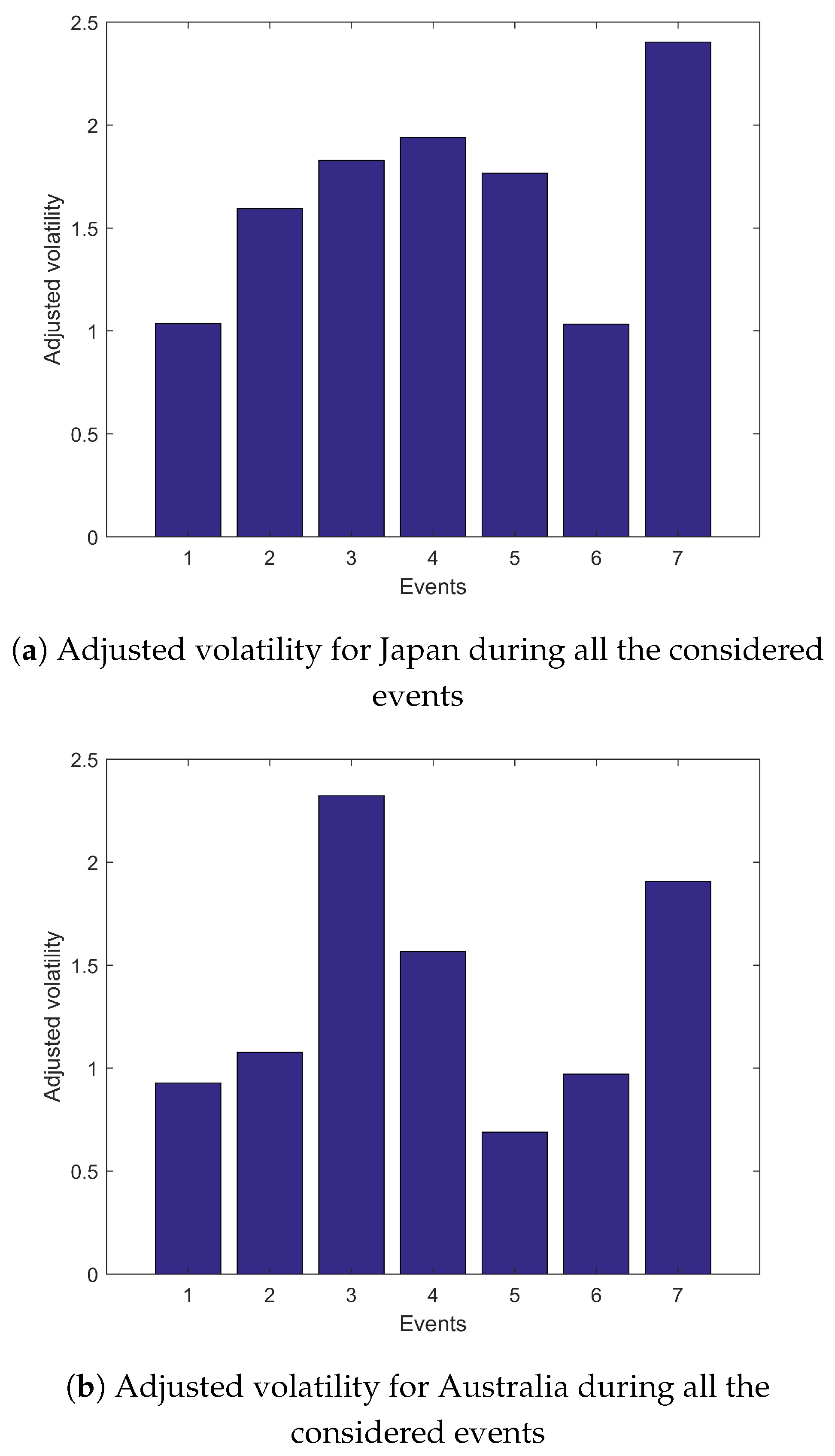
The results suggest that there are three distinct phases, from a stock market volatility point of view. Initially, the crisis was mostly regional in nature (event 1), mostly impacting emerging markets in South-East Asia. Volatility started to spread to other markets, such as for instance Japan (
Figure 1a) and even developed markets as different as Australia (
Figure 1b). This process reached its peak approximately at event 4. After that initial phase of increasing volatility (from event 1 to 4), volatility started to gradually return more normal historical levels. Volatility then experienced another spike during event 7. The results illustrated graphically with the adjusted volatility values were formally tested using F-tests. As previously mentioned the volatility for each event and each index was compared to the volatility during the base line period (1996). The result of the graphical approach and the formal statistical test are consistent with all the markets analyzed having statistically higher volatility during events 3, 4 and 7 compared to their base line levels.
In order to estimate a base line the pre-existing (1996), Granger relationships were analyzed. During this period, the stock market of the countries in the region did not appear, according to the Granger analysis, to be a major driver of other markets. For example, Indonesia was only driver (Granger causality) of the Hong Kong and Portugal markets (using 2 day lag) and the Philippines was only a driver of the Thai market. Hong Kong was a driver of Argentina, Indonesia, and the Netherlands, and Japan of Austria, Indonesia, and the Netherlands. Some of these Granger relationships might be the result of spurious data relationships not based on strong underlying economic reasons however some of those relationships seem consistent with expectations, such as for instance, Philippines and Thailand. Similar results were obtained when the analysis was carried out with 2 and 3 days lag. Overall, there were less than expected pre-existing relationship (Granger causality) among countries in the South-East Asia region. In the following sections the results for each event are presented.
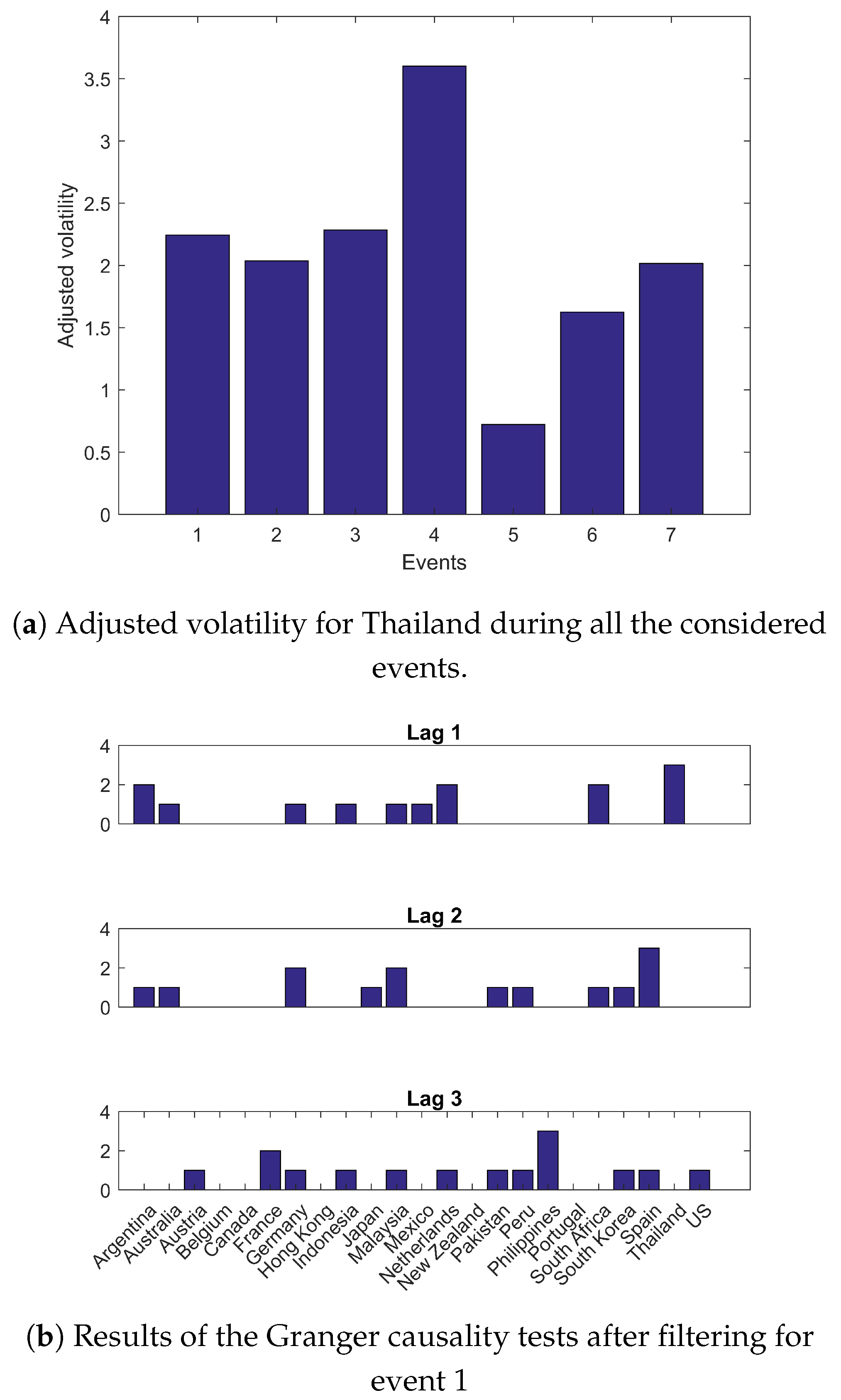
4.1. Event 1—2 July 1997
Thailand letting the Thai baht to freely float is arguably one of the most important event during the South-East Asia financial crisis. The results from the F-tests (
Appendix A Table A17) comparing the volatility of the stock markets suggest that at this stage the South-East Asia financial crisis was mostly a regional event. The volatility during this event was statistically higher than in the baseline period (1996) only in 6 out of the 24 countries analyzed, most of these countries where the volatility was significantly higher were countries directly related to the crisis such as Thailand and the Philippines. As illustrated in
Figure 2a, Thailand, since event 1, started having high adjusted volatility levels of almost twice its base line levels. This is a reasonable result considering that letting the Thai baht to float, after a long period of stable exchange rates, likely substantially impacted the performance of the Thai stock exchange. In
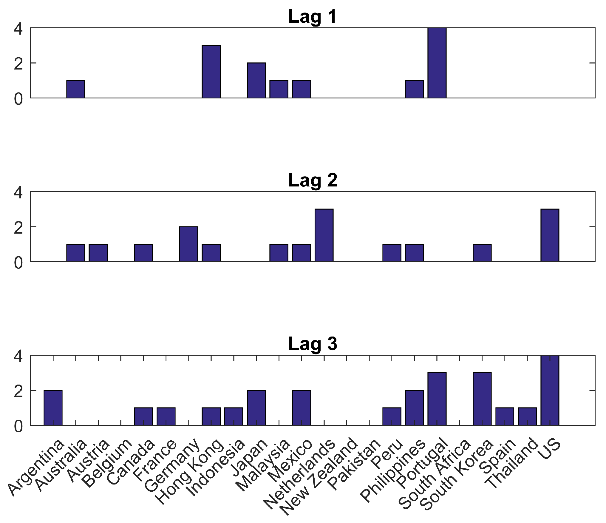
Figure 2b it is shown the results from the Granger causality tests (adjusted for baseline effects) using three different time lags (1, 2, and 3 days). The number of statistically significant Granger causality relationships was relatively low. Using 1 and 2 days lag there were only 14 statistically significant Granger causality relationships while 15 relationships were found when using 3 days lag. Interestingly during this first event, the Thai stock market, according to the Granger causality test, did not substantially impact other markets after adjusting for base line relationships. Perhaps this is related to investors, at that initial stage, considering that it was mostly a local issue. The stock market of Malaysia seems to have impacted, during this period, the stock market of Thailand (1-day lag) and Japan (2- and 3-day lag).
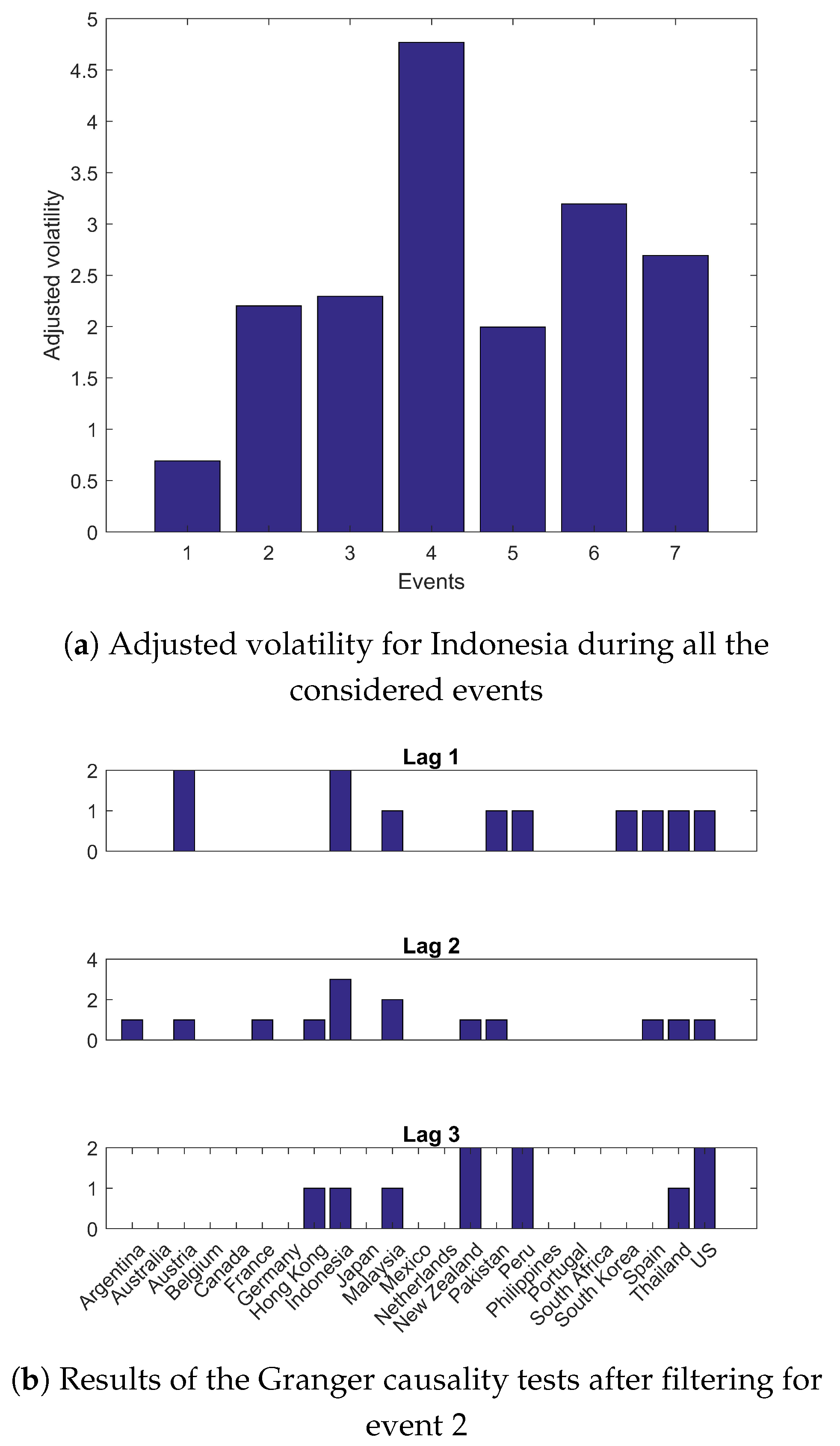
4.2. Event 2—14 August 1997
After several attempts to defend its currency on 14 August 1997, Indonesia decided to float its currency. The Indonesian Central Bank tried robustly to defend its currency but pressure was gradually increasing and foreign reserves were not large enough. Indonesia was initially not too severely affected. In fact, at the beginning of the financial crisis it was considered a success story. However, that rapidly changed with volatility doubling compared to its baseline level during the event 2 period. In the Indonesian case, volatility remained elevated for prolonged periods of time. The stock market experienced the same phases as previously mentioned with an initial phase of sustained volatility increases, peaking in event 4, followed by a phase of lower volatility, around event 6. The main difference in the Indonesian case compared to some other markets is that this phase of lower volatility was shorter with a volatility spike during event 6. Volatility remained high during event 7. The number of Granger causality relationships remained low during this period at 11, 14 and 10 for lags of 1, 2 and 3 days, respectively (
Figure 3).
4.3. Event 3—14 October 1997
In 14 October 1997, Thailand announced a restructuring package in another of the major events during the South-East Asia financial crisis. In this event volatility remained high compared to historical levels. In fact, from event 1 to 3 volatility was roughly twice the base line levels volatility of 1996. The number of statistically significant Granger causality relationships was one of the lowest during this period with only 10, 10, and 17 relationships identified when using 1-, 2-, and 3-day lag, respectively. A bidirectional relationship between the stock markets of South Korea and Indonesia was identified when using the Granger test (3-day lag).
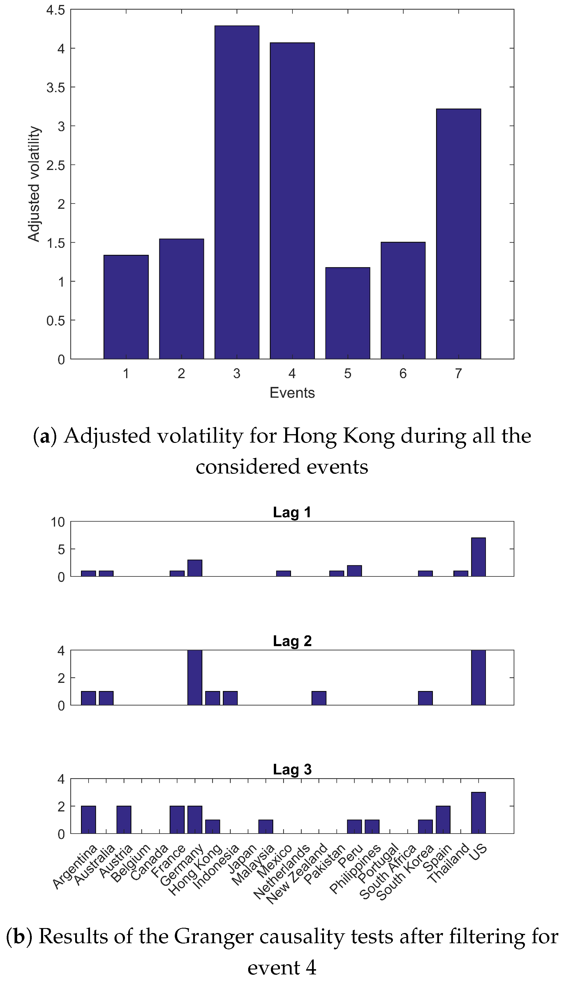
4.4. Event 4—12 January 1998
Another important event during the financial crisis was the collapse of Peregrine investment on 12 January 1998. The investment company was based in Hong Kong but it failed due to losses for a transaction in Indonesia. As it can be seen in
Figure 4a volatility in the Hong Kong stock market was significantly higher than the base line levels during events 3 and 4. Note that Hong Kong did manage to successfully defend its peg to the U.S. dollar but clearly its stock market was substantially impacted by the crisis. The same phases as in other markets can be identified in Hong Kong with a primary spike in volatility around event 3 and 4 and a secondary spike around event 7. As shown in
Figure 4b, the Indonesian market experienced a drastic increase in volatility in event 4 passing from approximately twice its baseline level in event three to more than four times during event 4. The number of Granger causality relationships identified as statistically significant (adjusted for base line level) remained relatively moderate during the event 4 period with 19, 14 and 18 relationships using 1-, 2-, and 3-day lags.
4.5. Event 5—31 March 1998
On 31 March 1998, another major development in the South-East Asia financial crisis happened with Thailand releasing new guidelines for the definition of nonperforming loans. Event 5 coincides with one of the lowest adjusted volatility periods for the markets analyzed. By event 5 there started to be clear, statistically significant signs of contagion among different stock markets with Granger causality relationships, adjusted by base line effects, increasing regardless of the lag used. The Granger causality relationship found using 1, 2 and 3 days lags were 34, 47, and 30, respectively (
Figure 5).
4.6. Event 6—11 May 1998
On 11 May 1998 Joseph Estrada won the general elections in the Philippines in another major development during the South-East Asia financial crisis. During this event volatility started to increase again compared to the previous events for most of the markets analyzed. The Granger causality tests identified 13 causality relationships among the countries, using a one-day lag period. When using 2 and 3 days lag there were 17 and 25 Granger causality relationships respectively (
Figure 6). A bidirectional relationships was found between the US and Canadian markets (3-day lag).
4.7. Event 7—3 September 1998
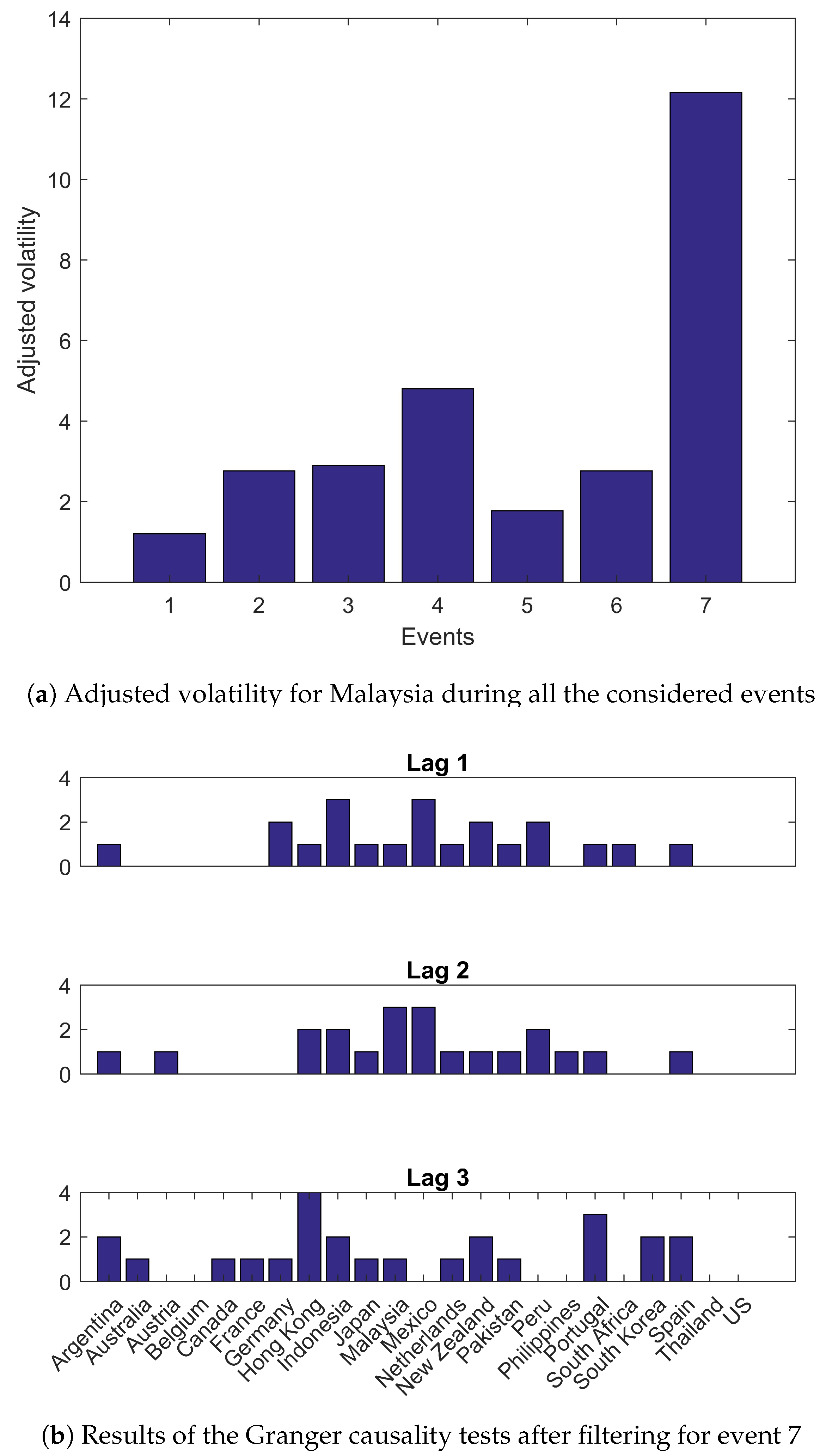
Event 7 was a rather important event with the replacement of the Malaysian finance minister. This event lead to a decades long feud among the Malaysian elites. As previously mentioned, Malaysia followed a rather unique direction during the crisis compared to its regional neighbors by refusing the bailout offered by the IMF. During event 7 most of the markets analyzed experienced a significant increase in volatility (
Figure 7a). The case of Malaysia is particularly remarkable with volatility increasing to 12 times the base line levels. This increase in adjusted volatility was much large in the case of Malaysia than in the case of its regional neighbors. Using one- and two-day lag there were 21 statistically significant Granger causality relationships while 25 relationships were found when using 3 days lag (
Figure 7b). The Indonesian stock market during this period seemed to impact several other markets such as for instance Japan and the Philippines (using a lag of 1 day). The adjusted volatility for all the countries/jurisdictions and for all the seven events considered can be seen in
Table A1. The main statistics for the indexes in 1996, which was used as a reference period to estimate the pre-existing (base) volatility of the indexes can be seen in
Table A2. The main statistics for the indexes for all the events can be seen in
Table A3,
Table A4,
Table A5,
Table A6,
Table A7,
Table A8 and
Table A9 and the results form the Granger tests can be seen in
Table A10,
Table A11,
Table A12,
Table A13,
Table A14,
Table A15 and
Table A16. The null hypothesis in the Granger tests is that
does not Granger cause
.
5. Discussion
When analyzing financial crises there is a tendency to consider the long term impacts on the economy with less attention to the short-term impacts on the equity market that are among the principal concerns for equity investors. Even if the equity market fully recovers after a financial crisis, the loss to equity investors might be very substantial. Equity investors might be forced to unwind the positions because risk management concerns or margin calls, even if they believe that the market is going to recover. This type of short-term fluctuations are sometimes neglected in the literature even if they might have very substantial economic impacts on investors.
While there is clearly some level of subjectivity, from a stock market point of view the South-East Asia financial market can be divided, according to the short-term event driven carried out, into three main phases. A first phase in which the crisis initially appears to be a local issue to then rapidly spread to other stock markets even outside Asia. This phase goes approximately from the decision of Thailand to float the baht on 2 July 1997 (event 1) to the collapse of Peregrine investments on 12 January 1998 (event 4). During this phase there is an increasing level of volatility, adjusted for base line effects, across stock markets. The number of statistically significant Granger causality relationships, adjusted for base line effects, also gradually increases. A second phase, of lower volatility across multiple stock markets happened during event 5 which was the release by Thailand of the new guidelines for non-performing bank loans on 31 March 1998. While volatility decreased during this period there are indications of contagion with the number of statistically significant Granger relationships increasing. This was a period of lower volatility that for some markets expanded to event 6. Event 6 was the victory of Joseph Estrada in the general elections of the Philippines on 11 May 1998. The final phase was another spike in volatility on 3 September 1998 when the Malaysian finance ministered was replaced triggering a spike in volatility across markets.
The results from F-test comparing the volatilities for each market during each event with its baseline levels of 1996 are consistent with above mentioned results. This analysis suggests that there were two differentiated peaks in stock market volatility one centered around the collapse of Peregrine investments (event 4) and another centered around the period when the finance minister in Malaysia was replaced (event 7). This second peak in volatility was, at least for some countries, even more intense that during the first phase of the crisis. During the period in which that Thai government released the new guidelines for non-performing loans classification (event 5) there were indications of contagion effects even outside Asia. There are, however, no statistically significant indications of a single country in South-East Asia having consistently driven (tested using Granger causality) the stock market of several other countries consistently during the entire crisis period.
It would be interesting, as a line of future research, to use machine learning techniques to model the stock prices during the Southeast Asia financial crisis. It remains unclear if machine learning techniques can handle black swan events such as the Southeast Asia financial crisis. Machine learning techniques use historical data to train the chosen algorithm, such as neural networks. If the behavior of the market during a financial crisis is new, i.e., the market has not experienced similar conditions in the past, the neural network might have problems generating accurate forecasts.


