Regime-Switching Determinants of Mutual Fund Performance in South Africa

Abstract

This study assesses the effect of fund-level and systemic factors on the performance of mutual funds in the context of changing market conditions. A Markov regime-switching model is used to analyze the performance of 33 South African equity mutual funds from 2006 to 2019. From the results, fund flow and fund size exert more predictive influences on performance in the bearish state of the market than in the bullish state. Fund age, fund risk, and market risk were found to be the most significant factors driving the performance of active portfolios under time-varying conditions of the market. These variables exert more influence on fund performance under bearish conditions than under bullish conditions, emphasizing the flight-to-liquidity assets phenomenon and risk-aversion behavior of fund contributors during unstable conditions of the market. Consequently, fund managers need to maintain adequate asset bases while implementing policies that minimize dispersions in fund returns to engender persistence in performance. This study provides novel perspectives on how the determinants of fund performance change with market conditions as portrayed by the adaptive market hypothesis (AMH).

1. Introduction

The investment focus of passive fund managers differs from active managers in terms of strategy and target clientele base. While passive management tracks the performance of a recognized market index or benchmarks, such as the New York Stock Exchange and the Johannesburg Stock Exchange, active management is premised on the ability to outperform the market (Cremers and Petajisto 2009; Cremers et al. 2016). However, drivers of fund performance could change with different market conditions, as suggested by proponents of the adaptive markets hypothesis (AMH) (Lo 2012; Al-Khazali and Mirzaei 2017). Explanations posited under the AMH suggest that the stability and efficiency of the financial markets in reflecting realistic values of financial assets is subject to change over time, and that investors and systemic fundamentals would adapt to prevailing conditions over the course of time (Lo 2012; Urquhart and McGroarty 2014). Consequently, the validation of AMH in the South African financial markets (Obalade and Muzindutsi 2018a, 2018b) suggests that the determinants of fund performance are subject to market conditions.

Evidence (S&P 2019) shows the prevalence of underperformance among fund managers in South Africa, where only 8.97% of active managers outperformed the market within five years (2014 to 2018). However, new investor assets continue to flow into the portfolios of fund managers, with over 1.9 trillion worth of assets under management as of the end of the second quarter of 2018 (Rangongo 2018). The mismatch between fund flow and performance results in the distortion of prices of assets and the efficiency of financial markets, which creates avenues for opportunistic traders to earn extraordinary returns. As a result, non-linear tools are required to test the dynamics of mutual performance, as much like other economic variables, the drivers of fund performance are subject to change over time.

However, the extant studies on mutual fund performance (Tan 2015; Arendse et al. 2018) were conducted in the context of stable market conditions, but these studies do not explain the enigmatic circumstances behind the increasing fund flows as against the continuous poor performance of mutual funds in South Africa, which can be explained by the current market conditions. In this context, the evaluation of the determinants of fund performance has to consider the dynamics of the market conditions because it provides additional analytical instrument for academics, investors, and industry practitioners who analyze mutual fund data for information and investment. Thus, this study makes significant contributions to the literature as the use of the Markov switching model in the forecasting of fund performance allows for regime dynamics to be accounted for to enable investors to achieve optimal returns on their investments relative to the associated risk of underlying assets.

The application of the Markov switching model in mutual fund performance analysis helps to measure the risk level in a given investment with two or more possible regimes or states of nature (De la Torre-Torres et al. 2020). Specifically, by knowing the probability of being in a given regime, an investor can determine whether to invest in a risky or riskless asset if the probability of being in a low volatility (bullish) or high volatility (bearish) regime of the market is high. Furthermore, a nonlinear analysis of the predictors of fund performance represents an important impetus towards eliciting explanations to incongruous flow-performance dynamics, explained in the preceding discussion. Moreover, the analysis of fund performance in the context of economic size provides additional perspectives on the effect of macroeconomic dynamics on fund performance under different market conditions. As a result, the main purpose of this study is to conduct a non-linear analysis of the determinants of South African mutual funds’ performance under bullish and bearish market conditions through a Markov regime switching framework. The study’s analysis tests the primary hypothesis that the dynamics of fund performance exert more predictive influences in the bullish state of the market than in the bearish state.

The remainder of the study is organized as follows: Section 2 presents the literature review, Section 3 presents the methodology and data sources, Section 4 discusses the estimation results of the empirical model, and Section 5 concludes.

2. Literature Review

Tan (2015) employs conventional measures of performance, namely the Sharpe, Treynor, Jensen’s alpha, Treynor and Mazuy (TM), and Henriksson and Merton (HM) indices, to assess the performance of mutual funds in South Africa in terms of returns and market timing experts. The results of the study show that despite the South African financial system’s resilience during the quantitative easing period after the global financial crisis in 2007/2008, most active managers recorded a benchmark trailing performance relative to optimal stock selection and market timing expertise. The conclusion of the study suggests a competitive fund stock market in South Africa post the global financial meltdown of 2007/2008, where less risk-bearing stocks generate similar returns, identical to high-risk ones. The findings of Tan (2015) generally provide insights about the determinants of mutual fund performance in South Africa.

However, the scope of the sample data (2009 to 2014) covering only the post-crisis period does not allow the dynamics of fund performance across different market conditions to be accounted for. Besides, the application of linear tests for the analysis of fund performance do not provide accurate explanations for the behavior of influencing factors of fund performance. This is because the dynamics of economic variables are subject to change to under different conditions. As a result, the use of nonlinear models, such as the Markov switching framework, which endogenously determines the different market regimes of a given time series, help to obtain more accurate inferences about the behavior of the influencing variables. Furthermore, the conventional performance measures employed in the analysis are prone to dynamic manipulation by fund managers (Qian et al. 2014). Hence, the reliance on these conventional metrics to test the performance of fund managers can lead to wrong conclusions about the performance of funds.

Arendse et al. (2018) investigated the generalized conclusion in the literature, intimating the existence of a positive relationship between the lagged performance of funds and the direction of subsequent fund flows in South Africa. The study employed a portfolio time-series technique, where funds were ranked according to their lagged performance over a period and grouped into quintiles. The evidence shows funds operating in emerging economies, such as South Africa, need to maintain superior performance momentum to sustain investor cash allocations to them. Additionally, the study documents that mutual fund contributors put more of a premium on funds’ superior performance compared to their competitors than fund performance relative to the market. In this context, the study concludes that mergers of funds represent a plausible means of sustaining the growth of the industry in South Africa. Overall, the findings of Arendse et al. (2018) portray the direction of growth of the South African fund industry. However, their conclusions are inadequate in explaining the flow-performance asymmetries under different market conditions, as the relationship between fund flow and performance was tested with linear tools in this study.

Using the Carhart (1997) four-factor model, Huij and Post (2011) investigated performance persistence among mutual funds in emerging markets, which included South Africa. The conclusion of the study suggests that funds operating in emerging economies generally exhibit superior performance compared to their counterparts in the US. Like other emerging equity fund markets, the South African fund industry generally exhibits persistence in performance while differing significantly in characteristics from equity funds of the US market (Huij and Post 2011). However, recent evidence by Bertolis and Hayes (2014) shows that the South African equity fund industry is gradually filtering out of persistence in performance relative to their counterparts in other emerging markets. Nonetheless, the lack of persistence in the performance of funds in South Africa is inconsistent with the continuous flow of investor assets to fund managers.

As explained in Section 1, fund managers in South Africa underperformed in the market consistently over five years (2014–2018). The evidence shows that the average performance, in terms of realized returns of South African funds, underperformed the market index by 34.01% in one year, trailed it by 84.66% in three years, and significantly underperformed it by 91.03% in five years (S&P 2019). Nonetheless, the volume of new cash inflows into South African equity mutual funds increased, with over R2.2 trillion assets currently under management (ASISA 2020). This evidence implies the existence of a significant mismatch in the flow–performance relations given the increasing level of investor allocations and the cross-sectional average performance of South African funds.

Arendse et al. (2018) further demonstrated that fund managers and contributors in South Africa exhibit traits of convex reactions relative to fluctuations in stock prices, and the level of risk assumptions vis-à-vis access to market updates on stocks of active portfolios. This phenomenon can be linked to the findings of Popescu and Xu (2017), which suggest that risk-shifting tendencies among active fund managers are indicative of less exposure bearing activity during bear markets and aggressive investment activity during bull markets. In this context, nonlinear test tools are required to analyze the flow–performance relations to generate accurate inference about the behavior of these economic variables under changing market conditions. Largely, the extant research on mutual fund performance dynamics in South Africa is premised on linear prepositions and methodologies driven by the underlying explanations of the EMH, and hence they are unable to provide explanations of the inscrutable dynamics influencing the continuous inflow of investor cash to consistently underperforming fund managers in South Africa (Arendse et al. 2018; Huij and Post 2011; Tan 2015).

However, explanations posited under the AMH suggest that the interaction between economic variables, such as fund flow and performance, is unlikely to be the same under different market conditions, as their behaviors are subject to change over time (Lo 2012). Besides, individual markets experience varying predictability levels attributable to market conditions (Urquhart and McGroarty 2016) and hence, nonlinear modelling of the market dynamics is required to ascertain accurate conclusions about the behavior of economic variables, such as the performance of fund portfolios. Bojanic (2021) explained that Markov switching models are mostly employed for the analysis of macroeconomic and financial variables as the dynamics of these variables are subject to periodic and systemic fluctuations over time. Pastpipatkul et al. (2020) also affirmed that Markov switching models help to account for dynamic change in economic data because the economic factors exhibit varying levels of dependencies under different market conditions. As explained in Section 1, the application of the Markov switching model in mutual fund performance analysis helps to measure the risk level in a given investment with two or more possible regimes or states of nature. In this context, an investor can determine whether to invest in a risky or risk-free asset if the probability of being in a bullish or bearish regime is high.

Furthermore, explanations for the consistent underperformance of fund managers despite the continuous flow of investors’ cash to them remain a gap in the literature that calls for an investigation. Moreover, with a projection of a significant rise in South African mutual fund assets due to a resurgence in stock investment in 2019 and beyond (Ziphethe-Makola 2017), knowledge of the influencing dynamics of performance under changing market conditions becomes an essential toolkit for fund contributors and fund managers for optimal investment decision-making. It is hypothesized in this study that fund-level and systemic factors exert more predictive influences on fund performance in bullish markets than in bearish market conditions.

3. Methodology

3.1. Data and Sample Selection

Quarterly data spanning from the end of first quarter of 2006 to the end of the last quarter of 2019 of 33 actively managed equity funds sourced from McGregor BFA Library, S&P Capital IQ, and the Association of Savings and Investment South Africa (ASISA) website were employed in this study. GDP data for economic size was sourced from the South African Reserve Bank’s website. For a fund to be included, it should have six years of data for analysis and the sample period was determined by the availability of data. In calculating South African equity funds’ performance, quarterly returns of the price index of funds were logarithmically computed. Following Rupande et al. (2019), fund performance by raw returns was formulated as:

$${\mathrm{R}}_{\mathrm{it}}=\ln ({\mathrm{P}}_{\mathrm{it}}/{\mathrm{P}}_{\mathrm{it}-1})\times 100$$

(1)

where ${\mathrm{R}}_{\mathrm{it}}$ is the return on fund i in quarter t, ${\mathrm{P}}_{\mathrm{it}}$ denotes the current price of fund i in quarter at t, ${\mathrm{P}}_{\mathrm{it}-1}$ is the price of the fund in the previous period t−1, and $\ln$ is the natural logarithm of the price index.

Following Nenninger and Rakowski (2014), fund flow was computed as the net quarterly percentage of cash flows accruing to a fund as a result of investor stock purchasing and redemption activity. A fund’s cash flow is expressed as:

$${\mathrm{Flow}}_{\mathrm{it}}=({\mathrm{TNA}}_{\mathrm{it}}-{\mathrm{TNA}}_{\mathrm{it}-1}(1+{\mathrm{r}}_{\mathrm{it}}))/{\mathrm{TNA}}_{\mathrm{it}-1}$$

(2)

where ${\mathrm{Flow}}_{\mathrm{it}}$ is the total net assets of fund i at quarter t, ${\mathrm{TNA}}_{\mathrm{it}}$ reflects the fund’s total net assets at quarter t, ${\mathrm{TNA}}_{\mathrm{it}-1}$ is fund i’s total net assets for the previous quarter t−1 whereas $r_{it}$ denotes fund i’s return in quarter t that accounts for reinvested dividends and adjusted for the fund’s overheads. Fund flow was included in the analysis as the main independent variable of interest because the literature suggests that funds that benefit from increased levels of cash flow generally perform better than funds that secured limited cash flow in the past (Rohleder et al. 2017).

3.2. Markov Switching Model for Determinants of Fund Performance under Bullish and Bearish Market Conditions

From the literature (Anas et al. 2007; Bilgili et al. 2012), Markov switching models are suitable for capturing the asymmetry and persistency in data with extreme values, while enabling accurate inference about the behavior of financial and economic variables within a nonlinear framework. Bilgili et al. (2012) attribute the extensive use of linear test tools in the analysis of financial data to the ready access to statistical software that are suited for predictive linear propositions. They explained that, notwithstanding the ability of linear models, such as bivariate or autoregressive integrated moving average (ARIMA), to account for the dynamics in economic and financial time series, their inability to capture dependency directions, volatilities, and asymmetries in the relationship of interacting variables remains a shortfall. However, Markov switching models enable parametric changes through stochastic innovations. In this context, fluctuations from bearish (high level volatility) to bullish (low level volatility) market conditions are accounted for through the estimation of the regime transition probabilities.

Prior studies (Gray 1996; Koy 2017; Ma et al. 2018) have applied the nonlinear econometric MS model of Hamilton (1989) for modelling nonlinear behavior of financial and macroeconomic time series. Fund performance, much like other economic variables, is subject to change over time and hence it requires nonlinear modelling to obtain accurate inferences about its behavior under different market conditions (Lo 2012). Kim (2004) explained that the Markov switching specification is appropriate for capturing the stylized dynamics of monthly and quarterly returns (Kim 2004). In addition, Markov-switching models define the market regimes endogenously, thereby avoiding the need to use instrumental variables and any data-mining concerns associated with doing so (Areal et al. 2013). Furthermore, Markov switching models account for possible structural breaks and regime changes in the behavior of economic variables, which allows for the estimation of the durations and probabilities of the innovations (Koy 2017). Although the use of high-frequency data allows for more data points for the regime switching analysis, the Markov switching model is applicable for the amount of quarterly data employed in this study, as Bilgili et al. (2012) employed quarterly data (spanning from the first quarter of 1988 to the second quarter of 2010) in Markov regime switching models to analyze the correlation between foreign direct investment (FDI) and a set of explanatory variables (11 variables in total).

Following Ma et al. (2018), a two-state Markov regime switching regression model (Hamilton 1989) was employed to estimate the determinants of performance ($y_{st})$ of individual funds in the cross-section. In this study, a two-state Markov switching model was estimated to ascertain how mutual fund performance is related to the set of explanatory variables employed in the analysis. Primarily, this model was estimated to capture and identify the effect of individual variables on fund performance under bullish and bearish conditions of the market. The adopted model is represented as follows:

$$y_{s_t}={\beta }_{0,s_t}+{\displaystyle \sum }_{i=1}^K{\beta }_{i,s_t}{x}_{i,t}+{\epsilon }_{s_t}$$

(3)

where $x_i\prime s$ are factors affecting the performance of a fund. The indicator variable $s_t=1$ or 2 denotes the two possible regimes’ switching states, which are unobservable, and ${\epsilon }_{s_t}$ is the normally distributed error term with zero mean and standard deviation ${\sigma }_{s_t}$ for each $s_t=1, 2.$

All the coefficients and the error term ${\epsilon }_t$ are allowed switch between the two states (bullish and bearish). The transition probability from state 1(2) to state 2(1) over the time period t to t+1 is governed by the Markov transition probability $p_{12}(p_{21})$, which is assumed to be constant over time. The distribution of $y_{s_t}$ is fully described by ${\sigma }_{s_t}$, ${\beta }_{0,s_t}$, ${\beta }_{i,s_t}$, $p_{11}$, and $p_{12}$ and 0 $<$ $p_{11}$ $<$ 1, 0 $<$ $p_{22}$ $<$ 1. The transition matrix P is therefore represented by:

$$P=[\begin{array}{cc}{p}_{11}& p_{12}\\ p_{21}& p_{22}\end{array}]$$

(4)

where $p_{11}$ + $p_{12}$ = 1 and $p_{21}$ + $p_{22}$ = 1.

Given that uncertainty surrounds the state of the market $s_t$ at any given time t, the state of the market $s_t$ is inferred from the state of the market at time t. The possibility of having $s_t$ at a given time t to be in regime j is given by:

$${\zeta }_{jt}=Pr(s_t=j{|\mathsf{\Omega }}_t;\theta )$$

(5)

where j = 1, 2, and ${\mathsf{\Omega }}_t$ is the information observed from time 0 up to time t including both the dependent variables and independent variables and $\theta$ is the set of population parameters of the regime switching regression; that is:

$$\theta =({\beta }_{i,1}, {\beta }_{i,2}, p_{11}, p_{12}, {\sigma }_1, {\sigma }_2)\prime$$

(6)

The regime of the state can either be 1 or 2. In this context, the two probabilities ${\zeta }_{1,t}$ and ${\zeta }_{2,t}$ always sum to 1. The probabilities can be inferred iteratively from t = 1, 2, …, T. Under Gaussian assumption of the error terms for the two regimes, the conditional densities needed to perform the iteration are given by:

$${\eta }_{j,t}=f(y_t|s_t=j, {\mathsf{\Omega }}_{t-1}; \theta )=\frac{1}{\sqrt{2\pi {\sigma }_j}} \exp [-\frac{{(y_t-x_t^{\prime }{\beta }_j^{\prime })}^2}{2{\sigma }_j^2}]$$

(7)

Thus, the conditional density of the observation is the probability weighted sum of both states, which is:

$$f(y_t| {\mathsf{\Omega }}_{t-1}; \theta )={\displaystyle \sum }_{i=1}^2{\displaystyle \sum }_{j=1}^2{p}_{ij}{\zeta }_{1,t-1}{\eta }_{j,t}$$

(8)

The log likelihood function associated with the iteration is then:

$$Logf(\theta )={\displaystyle \sum }_{t=0}^T\log f(y_t{|\mathsf{\Omega }}_{t-1}; \theta )={\displaystyle \sum }_{t=0}^T\log ({\displaystyle \sum }_{i=1}^2{\displaystyle \sum }_{j=1}^2{p}_{ij}{\zeta }_{i,t-1}{\eta }_{jt})$$

(9)

The parameters $\theta$ can be estimated by maximizing the log likelihood function of Equation (9).

To capture all the information available in the sample, the smoothed transition probabilities for the fluctuations in fund performance were estimated. This study follows Yu and Kobayashi (2006) based on the algorithm of Kim (1994) and mathematically represents the smoothed probabilities as:

$$P(S_t=i|S_{t+1}=j, {\mathrm{Ƶ}}^T; \theta )$$

(10)

$$\approx P(S_t=i|S_{t+1}=j, {\mathrm{Ƶ}}^t; \theta )$$

(11)

$$=\frac{P(S_t=i|S_{t+1}=j, {\mathrm{Ƶ}}^t; \theta )}{P(S_{t+1}=j |{\mathrm{Ƶ}}^t; \theta )}$$

(12)

$$=\frac{P_{ij }P(S_t=i|{\mathrm{Ƶ}}^t; \theta )}{P(S_{t+1}=j |{\mathrm{Ƶ}}^t; \theta )}$$

(13)

For i, j = 0, 1, thus the smoothed probabilities are given as:

$$P(S_t=i|{\mathrm{Ƶ}}^T; \theta )$$

$$=P(S_{t+1}=0|{\mathrm{Ƶ}}^T; \theta ) P(S_t=i|S_{t+1}=0, {\mathrm{Ƶ}}^T; \theta )+P (S_{t+1}=1| {\mathrm{Ƶ}}^T; \theta ) P(S_t=i|S_{t+1}=1, {\mathrm{Ƶ}}^T; \theta )$$

(14)

$$\approx P(S_t=i| {\mathrm{Ƶ}}^t; \theta )\times \left(\frac{P_{i0}|P(S_{t+1}=0|{\mathrm{Ƶ}}^T;\theta )}{P(S_{t+1}=0|{\mathrm{Ƶ}}^t;\theta )}+\frac{P_{i1}P(S_{t+1}=1|{\mathrm{Ƶ}}^T;\theta )}{P (S_{t+1}=1|{\mathrm{Ƶ}}^t;\theta )}\right)$$

(15)

Equation (16) depicts the model specification, where fund-level and systemic variables, namely fund flow, fund size, fund age, fund risk, market risk, and economic size, are employed as explanatory variables. The model is specified as follows:

$$PER{F}_{s_t}={\beta }_{0,s_t}+{\beta }_{1,s_t}FLO{W}_{i,t}+{\beta }_{2,s_t}LNTN{A}_{i,t}+{\beta }_{3,s_t}LNAG{E}_{i,t}+{\beta }_{4,s_t}STDFN{D}_{i,t}+{\beta }_{5,s_t}STDMK{T}_{m,t}+{\beta }_{6,s_t}ECOSIZ{E}_{m,t}+{\epsilon }_{s_t}$$

(16)

where $PER{F}_{s_t}$ is fund performance at time t and $FLO{W}_{i,t}$ is the total net assets of fund i at quarter t. Fund flow is included in the analysis as the main independent variable of interest because the literature suggests that funds that benefit from increased levels of cash flow generally perform much better than funds that secured limited cash flow in the past (Rohleder et al. 2017). Further, explanations posited in the smart money hypothesis suggest that fund contributors are able to distinguish between competent and incompetent fund managers, which informs their asset allocation decisions in favor of competent managers (Elton et al. 1996; Ferreira et al. 2013). In this context, it is generally expected that investor cash flows will exert a positive influence on the future performance of funds, although evidence suggests that the smart money hypothesis largely thrives on momentum as investors chase recent outperformers (Sapp and Tiwari 2004). $LNTN{A}_{i,t}$ denotes fund i’s size in quarter t, which is measured as the natural logarithm of total net assets. This variable was included in the analysis to control for the growth potential of funds, as large funds are generally more challenging to grow (Sirri and Tufano 1998; Guercio and Reuter 2014).

However, large funds attract more attention in terms of cash flow from investors, which results in a superior performance in the long run (Goetzmann and Peles 1997; Kacperczyk et al. 2016). Furthermore, scholars have explained that the maintenance of large volumes of investor assets result in a host of trading opportunities for fund managers (Ferreira et al. 2013). Evidence has shown that unlike small funds, large mutual funds benefit from economies of scale as they are able to minimize the per unit cost associated with their transactions and operations, while achieving optimal trading results (Ferreira et al. 2012, 2013). $LNAG{E}_{i,t}$ is the age of fund i at quarter t measured as the natural logarithm of the fund’s age in years. From the literature, the age of funds affects their overall performance as investors’ decisions on mutual funds are affected by the number of years a given fund has been in operation as older funds generally grow more slowly than younger funds (Del Guercio and Tkac 2002; Pástor et al. 2015). As a result, this variable was incorporated in the analysis to control for the effect of fund age on performance.

Following the formulation of Xiao et al. (2014), $STDFN{D}_{i,t}$ represents fund i’s portfolio risk at quarter t, and is measured as the standard deviation of a fund’s monthly returns from quarter t$-$4 to quarter t$-$1. This approach allows for the calculation of the annualised standard deviation (rate of dispersion) of fund returns in the past 12 months, and hence the riskiness of a fund’s portfolio. From the literature, the average investor is generally sensitive to the risk associated with an investment and takes it into consideration when making decisions on mutual funds, as fund risk adversely impacts their performance (Huang et al. 2012; Xiao et al. 2014). $STDMK{T}_{m,t}$ denotes market risk in quarter t, which is measured as the standard deviation of the stock market’s daily returns from quarter t$-$4 to quarter t$–$1. This method allows for computation of the annualized standard deviation of the daily returns of the stock market in the past trading year, to determine the overall risk of the equity market. Scholars have explained that stock market volatility affects investors’ decision on mutual funds, as investor skepticism about expected returns vis-à-vis the system risk increases under conditions of uncertainty (Barber et al. 2016; Kim 2019). $ECOSIZ{E}_{m,t}$ denotes the economic size (proxied by gross domestic product–lgdp) of the market in which fund i operates at quarter t. From the literature, the performance of mutual funds is linked to the direction of growth of the economy within which funds operate, where macroeconomic expansions impact positively on fund returns while economic contractions deteriorate the returns of funds (Ferreira et al. 2012; Fuerst and Matysiak 2013; Gueddoudj 2018).

In the analysis, a two-state regime switching regression model was used, where all coefficients and error terms are allowed to take on different values in the two states denoted by $S_t$. A bullish market condition is characterised by a general increase in market returns and low volatility, while a bearish market condition refers to the period of a downward spiral in market returns and high volatility. The adopted regime switching model was estimated for each fund in the sample. Eviews 12 software was used for the estimation of the empirical model.

3.3. Normality Tests

A normality test was conducted to analyze the sample data with a non-normal distribution for the results of the specified nonlinear model to be valid (Schmidt and Finan 2018; Tsagris and Pandis 2021). All the variables report some negative asymmetry in their dynamics (skewness) and none of the variables report a value of zero. Besides, all the seven interacting variables employed in the analysis show excess kurtosis across the sampled funds, as their reported kurtosis values were either below or above three. As a result, the Jarque-Bera (JB) tests reject the hypothesis of normal distribution. Consequently, non-normality is not a problem in the estimated models. It could be concluded that the results generated are valid in providing explanations to the dynamics of fund performance under different market conditions. The results of the normality test can be seen as Table S1.

3.4. Unit Root Tests

The presence of non-stationary explanatory variables is likely to lead to spurious regression when the MS model parameter is estimated (Granger and Newbold 1974). To resolve this problem, the augmented Dicky Fuller (ADF) was employed to check for the presence of unit roots for each selected variable for each fund in the sample. The ADF test shows that the variables employed in the analysis are all stationary across sampled funds. The unit root test results can be seen as Table S1.

4. Estimation Results and Discussion

4.1. Descriptive Statistics of Fund Performance

Table 1. Descriptive statistics of fund performance.

Fund	Mean	Medium	Maximum	Minimum	Standard Deviation	Skewness	Kurtosis
Afena	1.921	2.857	8.594	−8.004	3.440	−0.933	3.393
Allan Gray	2.107	1.848	16.238	−14.326	5.218	−0.304	4.135
4D BCI	2.160	1.856	11.966	−4.688	3.317	0.151	3.304
3LAWS	−0.073	1.000	5.000	−7.000	3.199	−0.468	2.154
3600ne	3.666	5.000	12.000	−16.000	5.548	−1.055	4.249
Aluwani	3.549	3.022	15.664	−6.487	5.780	0.108	2.240
Analytics	2.232	3.449	6.953	−6.934	2.982	−1.317	4.266
Anchor	2.877	4.207	12.028	−6.939	3.592	−0.376	3.540
Blue Alpha	1.864	2.423	9.873	−7.095	3.813	−0.055	2.582
Bridge	3.469	4.030	12.029	−6.939	3.574	−0.539	2.235
Cannon	1.162	1.068	16.058	−9.937	5.517	0.554	3.631
Capita BCI	1.427	1.708	3.604	−3.479	1.435	−1.509	6.067
Centeaur	2.779	4.186	15.415	−15.706	6.282	−0.890	4.182
Clucasgray	0.789	0.686	10.431	−6.164	2.836	0.394	4.558
Counterpoint	0.553	0.644	4.478	−3.746	1.535	−0.081	3.853
Dalebrook	0.275	0.290	6.301	−7.118	3.068	−0.415	3.332
Denker	0.363	0.389	4.478	−3.746	1.565	0.196	3.626
Graviton	1.699	2.276	3.360	−3.619	1.454	−1.656	5.738
GTC	0.114	0.038	6.454	−6.899	2.618	0.034	4.161
Harvard	0.006	0.103	6.241	−10.738	2.605	−1.347	7.701
Huysamer	0.459	−0.157	8.651	−11.155	3.779	−0.183	3.450
Imara	2.288	2.546	9.746	−8.524	3.716	−0.381	3.564
IP HIGH	−0.927	−1.034	8.499	−7.946	2.905	0.562	4.427
Kagiso	3.382	3.595	25.093	−9.032	6.054	0.895	4.998
Maestro	0.484	0.205	7.343	−10.719	3.479	−0.587	3.919
Naviga	−0.092	−0.141	6.285	−6.419	2.259	−0.007	4.959
Northstar	2.462	2.364	15.992	−8.701	3.733	0.808	6.745
Personal Trust	−0.286	0.078	8.980	−9.588	3.139	−0.381	5.003
RCI	1.539	2.870	10.244	−12.306	4.598	−1.031	4.144
RECM	1.238	2.146	14.368	−15.618	4.907	−0.922	5.689
Stanlib	4.012	4.045	13.084	−5.799	4.374	−0.093	2.529
ABSA Prime	3.410	3.520	13.083	−5.798	4.089	0.104	2.728
Prescient	3.792	6.101	9.240	−6.935	4.582	−0.929	2.401

Source: Authors’ estimations (2021).

summarizes the descriptive statistics of the levels of quarterly performance of the 33 sampled funds for the period March 2006 to end of 2019. From the table, the performance varied considerably across the funds, with IP HIGH fund being the lowest (with a mean value of −0.927) and Stanlib fund being the highest (with a mean value of 4.012). The variation in the performance of each fund during the period under study appears to be significant as can be observed from the large difference between the maximum and minimum performance values. The variation in cross-sectional performances is largely linked to the period of financial meltdown in 2007 and 2008, where it is found to be more evident. Moreover, the performance of the funds shows several negative asymmetries in their dynamics (skewness) and excess kurtosis is reported across the sampled funds, implying that the performance of the sampled funds is not normally distributed. In this context, it can be explained that the performance of the sampled funds lacked stability.

4.2. Discussion of Markov Regime Switching Regression Results of Fund Performance Determinants

Table 2. Markov regime switching regression results summary of fund performance determinants.

Fund	Intercept	FLOW	LNTNA	LNAGE	STDFND	STDMKT	ECOSIZE
Afena	11.938 *** 5.479 ***	−0.072 0.224 ***	0.058 −1.232 ***	−2.068 *** −0.818 ***	−643.486 *** −93.279	−0.706 ** −0.205	−0.127 ** −0.099
Allan	2.078 12.712 ***	−0.034 −0.062 **	0.709 *** −0.513 ***	−2.204 *** −2.534 ***	71.376 97.015	−2.151 *** −2.338 ***	−0.142 ** 0.048
4D BCI	8.924 *** 1.086	0.106 −0.007	0.296 −0.177	−2.805 *** 0.338	−35.376 103.763 *	−4.034 *** −0.566	0.058 −0.010
3LAWS	12.113 15.862 ***	0.057 −0.001	−0.706 1.052 ***	−6.016 −10.195 ***	80.598 −152.805 ***	−5.656 *** −0.935 ***	0.439 * −0.076
360One	23.914 *** 13.486 ***	0.464 0.091	0.124 −1.709	−9.207 −0.055	−2167.139 *** −1204.542 ***	0.331 4.485 **	−1.099 −0.426
Aluwani	6.600 *** −3.635 *	0.009 *** −0.001	−0.717 * 0.435	−0.556 ** −0.454 *	118.190 120.512 ***	−2.124 −2.298 ***	−0.007 0.063
Analytics	20.298 *** −1.609	−0039 ** −0.009 ***	−1.267 *** 0.123	−4.964 *** 0.644	55.642 0.685	−0.418 0.223	0.027 0.167
Anchor	9.284 *** 12.411 ***	−0.017 0.287 ***	−0.547 −1.103 ***	−0.360 0.746 ***	−534.978 *** −601.861 ***	−0.353 −3.639 ***	0.018 0.139 ***
Blue Alpha	3.816 17.628 ***	0.019 0.014 **	0.042 −3.062 ***	−2.015 * −0.095	51.544 *** −204.309 ***	−0.344 8.387 ***	−0.307 −0.015
Bridge	41.411 *** 51.252 ***	0.033 −0.244 ***	−4.758 *** −4.366 ***	−1.126 −1.292 ***	−872.245 *** −711.282 ***	1.017 −12.949 ***	0.705 −1.321 ***
Cannon	29.533 *** −10.563 ***	0.275 −0.479 ***	−2.791 3.859 ***	−25.581 *** 2.836	1035.957 * −405.872 ***	−23.252 *** −6.390 ***	−0.635 −0.064
Capita BCI	6.100 *** −0.488	0.037 0.013	−0.852 −0.026	−0.812 *** 0.048	−596.041 *** 372.714 ***	−3.136 *** 0.071	0.012 0.008
Centeaur	5.220 *** 7.291 ***	−0.058 −0.216 ***	−0.134 0.379	−0.681 −2.770	119.551 *** −162.205 ***	−1.783 *** −2.238 ***	0.126 −0.433 ***
Clucas.	3.427 *** 1.814	−0.227 *** −0.156 ***	−0.143 −0.013	−1.043 *** 0.375 **	13.954 −77.569	−0.346 −0.216	−0.168 *** −0.017
Counter.	−0.797 1.314 ***	0.017 *** 0.008 *	0.174 −0.125	−0.664 0.454 ***	102.463 *** −11.537	−0.895 −0.349 ***	0.077 0.029
Dalebrook	−2.834 * 7.903 ***	0.006 *** −0.014 ***	0.602 *** −0.661 ***	0.125 −1.338 ***	−27.726 −390.159 ***	0.597 −1.407 *	−0.044 0.794 ***
Denker	1.302 −4.237 ***	0.003 −0.002	−0.169 −0.241	0.406 *** 0.459	4.206 635.442 ***	−0.251 −0.425 *	0.014 0.215 ***
Graviton	4.633 1.365 ***	0.069 0.008	−0.017 −0.091 ***	−0.909 0.105	−209.823 29.489	−1.718 *** 0.017	0.134 ** 0.025 ***
GTC	24.858 21.647 ***	−0.034 −0.030 ***	−2.135 * 1.434 ***	−4.037 −6.902 ***	−632.123 * −223.809 ***	−8.683 *** 1.551 *	−0.251 0.148
Harvard	−1.953 −3.216 **	−0.127 *** 0.043	2.457 *** 1.214	−0.191 0.826 ***	−466.652 *** −21.239	0.682 * 0.336	0.256 0.093
Huysamer	−4.197 0.810	0.136 *** 0.012	2.598 *** −0.995	0.038 0.446	54.873 * 21.280	−1.054 0.481	0.088 0.350 ***
Imara	−5.442 * 1.340	0.006 * −0.001	2.104 *** 0.911 *	0.802 −0.154	−237.013 *** −181.277 ***	1.003 *** 0.347	0.089 −0.001
IP HIGH	11.217 28.931 ***	0.007 0.002	−4.816 −19.534 ***	−1.721 *** 5.988 ***	−370.190 ** −268.682 ***	0.739 5.809 ***	−0.033 0.850 ***
Kagiso	7.737 *** 7.358 ***	0.038 −0.037 ***	−0.561 −0.469 ***	−1.207 −1.242 ***	15.936 137.428 ***	−5.123 *** −3.951 ***	−0.252 ** −0.125 ***
Maestro	4.174 *** 1.042	−0.325 *** 0.123 ***	0.921 *** −0.452 ***	−2.969 *** 0.723	−130.129 −254.010	−0.124 2.430 *	0.267 * −0.180
Naviga	3.042 −6.046 ***	−0.019 * −0.220 ***	−0.226 2.355 ***	−0.886 * −1.827 ***	100.498 617.188 ***	−0.778 −6.677 ***	−0.486 3.208 ***
Northstar	7.624 *** 7.459 ***	−0.009 0.069 ***	2.225 ** 4.282 ***	−3.485 *** −5.145 ***	123.799 −3.175	−0.355 −0.759 ***	−0.089 * 0.102 ***
Personal Trust	−1.082 −4.345 ***	0.053 *** −0.001 ***	1.767 * 2.867 ***	−0.487 −0.831 ***	−58.519 28.875	−0.485 −0.813 ***	−0.238 −0.218 ***
RCI	46.592 * 48.343 ***	0.007 0.053 ***	−14.441 −18.791 ***	−10.574 * −11.566 ***	−69.376 −791.605 ***	−4.146 *** 1.157 ***	−1.116 2.643 ***
RECM	0.433 −0.535	−0.072 0.058 *	0.619 0.129	−1.366 0.416 ***	−379.661 *** 108.669 ***	2.130 ** −0.130	−0.425 * −0.066
Stanlib	18.676 *** 32.022 ***	−0.039 0.039	−3.532 * −5.235 ***	2.503 1.834 ***	−342.103 −704.414 ***	8.067 3.089 ***	−0.206 0.307 ***
ABSA	14.788 *** 33.219 ***	−0.001 0.024 ***	−1.801 −0.404	−1.665 −6.777 ***	−369.628 −784.171 ***	3.493 −1.549	0.035 −1.269 ***
Prescient	5.137 9.116 ***	0.004 −0.028 ***	9.511 *** 13.604 ***	−6.716 *** −9.491 ***	−433.241 −973.846 ***	3.344 8.023 ***	0.144 −0.384 ***

Note: *, **, and *** denote 10%, 5%, and 1% levels of statistical significance respectively. Source: Authors’ estimations (2021).

presents a summary of the Markov regime switching regression (Equation (16) results of fund performance determinants for sampled funds. The first row of each fund reports the estimated coefficients for the bullish Markov state and the second row reports those of the bearish state.

From Table 2, it can be observed that fund-level and systemic variables exert varying influences on fund performance across bullish and bearish market conditions. Fund flow reports more significant relationships (23: 10 positive and 13 negative values) with performance across funds in the bearish state of the market, as against 10 (six positive and four negative values) significant coefficients in the bullish state. This result shows that fund flow, under the regime switching environment, exerts more influence on performance under bearish conditions of the market than under bullish market conditions. The results thus indicate that the high sensitivity of fund flow to performance in the bearish market is more in the negative terms than positive. This evidence is consistent with the position of the extant literature. Kosowski (2011) applied a Markov switching approach to analyze the determinants of fund performance and found that the effect of fund flow on performance is more evident in the bearish regime of the market than in the bullish regime. The study documents a negative predictive power of fund flow over performance, and explains that overtrading on the part of recent outperformers with enhanced investor cash allocations results in operational overruns that are not appropriately compensated for due to an increase in market volatility.

The results of Papadimitriou et al. (2020) also verify that the flow–performance relationship is more pronounced under bearish market conditions than bullish conditions. Moreover, Franzoni and Schmalz (2017) explained that investor risk-aversion tendencies and skepticism about fund performance during lower periods of the market tend to be more informative about managers’ trading skill, compared to performance during upper periods of the market. However, Xiao et al. (2014) found that the sensitivity between fund flow and performance is more evident in the bullish state of the market than in the bearish state. They explain that generally, the effect of fund flow on performance is positive under changing market conditions and attribute this state of interaction to an increase in investor confidence in the trading skills of fund managers in bullish market conditions than in bearish conditions.

From Table 2, fund size (proxied by the natural logarithm of total net assets) reports more significant coefficients (20: 8 positive and 12 negative values) across the sampled funds in the bearish state than in the bullish state (13: eight positive and five negative values). This result implies that the influence of fund size on performance is more evident under bearish market conditions, and it is generally adverse under bullish conditions. From the literature, it is suggested that investor decisions regarding mutual funds are affected by fund size as large funds are generally more challenging to grow (Chevalier and Ellison 1997; Sirri and Tufano 1998; Xiao et al. 2014). Given that bearish market conditions are generally characterized by increased volatility and uncertainty around expected returns on underlying investment, it is expected that investor attention will focus more on the disadvantages associated with the acquisition of large funds’ stocks (Chou and Hardin 2014). Similarly, through the application of a regime switching framework, Badrinath and Gubellini (2012) found that on a comparative basis, small funds are able to achieve higher returns than large funds under changing market conditions, which is more evident in bearish conditions of the market. However, the regime switching results of the drivers of fund performance by Chung et al. (2014) show that the predictive power of fund size over performance is more pronounced in the bullish state of the market than in the bearish state. Their finding links the effect fund size on performance to positive investor sentiments of fund managers’ trading expertise. They explain that skepticism about the pace of growth of a fund is given minimal consideration by investors during stable market conditions, and hence they allocate more cash to large funds with the expectation of benefiting from wider investment opportunities.

The fund age variable (proxied by the natural logarithm of fund age in years) shows a more significant relationship with performance in the bearish state (21 significant coefficients: 14 positive and 7 negative values) than in the bullish state (16 significant coefficients: 1 positive and 15 negative values) across the sampled funds. Given that the significant relationship between fund age and performance is generally positive, it suggests that investors’ cash allocation decisions on mutual funds are largely in favor of old and more established funds. However, the Markov switching results of fund performance determinants by Stafylas and Andrikopoulous (2019) suggest that young funds are generally able to sustain superior performance momentum during market downturns compared to their older counterparts. Similarly, evidence from other studies (Pástor et al. 2015; Rao and Tauni 2016) indicates that investor decisions on mutual funds favor younger funds, as older funds grow at a slower pace than younger funds. Meanwhile, the findings of a regime switching analysis of fund performance link the time-varying effect of fund age on performance to investor sentiments (Chung et al. 2014). The study explained that the effect of investor sentiment on fund performance is more pronounced in the bullish state of the market than in the bearish regime when it is driven by considerations premised on fund age and the ability to expand rapidly.

From Table 2, it can be observed that the influence of fund risk (proxied by the annualized standard deviation of funds monthly) on performance is generally pronounced in the bearish state (23 significant coefficients: 8 positive and 10 negative values). The bullish regime reports 15 significant coefficients (5 positive and 10 negative values). This result is expected because increased variability in fund returns tends to diminish investor confidence in fund managers’ ability to generate utility for investors, as the literature (Li et al. 2013) suggests that mutual fund contributors take portfolio risk into consideration when making stock-picking decisions on mutual funds. In this context, the performance of funds with significant levels of risk are adversely affected as minimal investor assets accrue to them. However, Chung et al. (2014) obtained Markov switching results for the effect of fund risk on performance under changing market conditions. Much like the evidence found for fund age, their results link the time-varying effect of fund risk on performance to investor sentiments. They explained that the average investor becomes less skeptical about fund return variability when market conditions are less volatile, regardless of the direction of the fund manager’s recent performance.

From the table, it can be observed that the market risk (proxied by the annualized standard deviation of daily returns of the equity market) exhibits a more significant relationship with performance in the bearish state (22 significant coefficients: 7 positive and 15 negative values) of the market than in the bullish state (13 significant coefficient: 2 positive and 11 negative values) across the sampled funds. This result suggests that generally, increased market volatility leads to significant deterioration of fund performance under time-varying conditions of the market. Through a Markov switching analysis, Turtle and Zhang (2012) found that the performance of funds operating in markets dominated by significant volumes of foreign investments tends to experience instability in performance as their activities are prone to the effects of fluctuations in external markets. Their evidence suggests that the performance of funds operating in emerging markets like South Africa experiences significant improvements in returns during periods of positive trends in the returns of advanced markets. These dynamics represent a spill-over market risk, which exerts significant impacts on the performance of emerging market funds as a result of their dependence on foreign investment. Intuitively, an increase in the dispersion of benchmark returns adversely impacts fund portfolios, as fund portfolios with significant components of its underlying investments deposited in exchange traded instruments are affected. Scholars have explained that investors’ cash allocation decisions on mutual funds are influenced by market risk, which, in turn, affects funds’ overall performance (Kim 2019; Barber et al. 2016).

As can be observed from the table, economic size shows a strong predictive influence on mutual fund performance under bearish market conditions (17 significant coefficients: 11 positive values and 6 negative values) than under bullish conditions (8 significant coefficients: 2 positive and 6 negative values). This evidence implies that generally, funds operating in large economies are able to perform better than their counterparts in smaller economies during periods of market downturns. This result is plausible because bigger economies present wider and more diverse trading opportunities for fund managers to relocate underlying investments in times of market meltdown to enhance performance. Kosowski (2011) applied the Markov switching approach to analyze the effect of economic fluctuations on fund performance and document that funds generally achieve more enhanced returns during periods of economic recession than expansion. Fund contributors thus exploit the time-varying risk-adjusted returns by allowing for predictability in performance. The study explained that fund contributors are able to benefit from predicted returns in this context because active managers are able to achieve significant excess returns during the contraction phase of the economy. In general, scholars agree that the performance of mutual funds is tied to the general well-being of the economy within which they operate (Ferreira et al. 2013; Fuerst and Matysiak 2013; Gueddoudj 2018). This appears to be the case in South Africa, indicating that stable economic growth is fundamental to the creation of a conducive environment for the growth of the South African fund market. Moreover, from the analysis, it can be observed that all the variables employed in the analysis exert more significant impacts on fund performance in the bearish state of the market than in the bullish. As a result, the study’s hypothesis that the impact fund-level and systemic factors on mutual fund performance are more pronounced in the bullish state than in the bearish state is rejected as per the results in Table 2.

Table 3. Cross-sectional analysis of the most significant explanatory variables.

Variable
Regime	LNAGE	No. of Funds	STDFND	No. of Funds	STDMKT	No. of Funds
S1	−4.249 ***	16	−358.263 ***	15	−2.563 ***	13
S2	−2.327 ***	21	−286.371 ***	22	−0.876 ***	21

Note: *** denotes a cross-sectional average statistical significance level at 1%. Source: Authors’ estimation (2021).

shows the average of the coefficients of these three variables (obtained from running the estimated regime-switching model of Equation 16 of the funds in the sample). The cells labelled S1 and S2 consist of results for the bullish and bearish states, respectively. The three variables are LNAGE, STDFND, and STDMKT. The discussion of the most significant explanatory variables follows the presentation of the results in Table 3 for ease of reference.

4.3. Cross-Sectional Analysis of the Most Significant Explanatory Variables

From the empirical analysis in the previous section (Section 4.2), it can be observed that all the explanatory variables have an impact on the performance of mutual funds in South Africa, where fund-level and systemic variables show greater influence in market downturns than in upturns. In addition, significant differences are observed among the sampled funds in terms of the extent to which these explanatory variables are linked with a fund’s performance. To ascertain the determinants of these cross-sectional differences, the three most significant explanatory variables were selected to conduct the cross-sectional analysis based on the regression results of Equation (16) as shown in Table 2.

The average coefficient of LNAGE for the cross-section of sampled funds in the bullish state (S1) is −4.24, which is composed of 16 funds with an average statistical significance at 1%. In the bearish state (S2), the average coefficient of LNAGE for the cross-section of funds is −2.327, which comprised 21 funds of the study sample and an average statistical significance at 1%. This evidence shows that fund age generally has a larger impact on fund performance in the bearish market (S2), which is consistent with the evidence of prior studies (Del Guercio and Tkac 2002; Xiao et al. 2014; Pástor et al. 2015) that investor decisions on mutual funds are affected by fund age, as downward spirals in general market returns pose a threat to the value of investor assets. Stafylas and Andrikopoulous (2019) analyzed the determinants of fund performance under different market conditions using a Markov regime switching framework. Their results, however, suggest that the predictive power of fund age over performance is more evident in the bullish state of the market than in the bearish state. They document that recently established funds generally exhibit superior performance in periods of low volatility relative to their older competitors in the industry, while a reverse of this state of performance holds for old and young funds during periods of high market volatility. Comparing the results for LNAGE of funds in the cross-section with the results of FLOW and LTNA in Table 2, it can be observed that most of the funds with significant coefficients for LNAGE in the bearish state also report significant coefficients for FLOW and LNTNA in the bearish state. This relationship is linked to the expected behavior of investors to be influenced by fund age and size when finalizing investment decisions on mutual funds.

Stafylas and Andrikopoulous (2019) verified that small and young funds are able to generate superior returns relative to old and large funds, even in bearish states of the market, and hence justifies investors’ favorable decisions on them under changing market conditions. The significance of coefficients of STDFND for funds in the cross-section is larger in the bearish state (22 significant coefficients; with most of them being negative) than in the bullish state (15 significant coefficients), which indicates that fund risk exerts a more retrogressive impact on the performance during periods of market decline. Based on the results of Markov regime switching regressions, Huang (2012) attributed persistence in fund return variability to inferior market timing ability over the business cycle on the part of active managers. It can be observed from the results shown in Table 2 and Table 3 that most of the funds with significant coefficients for STDFND also report significant coefficients for FLOW and LNTNA. This evidence explains that investors’ cash allocation decisions on mutual funds are influenced by portfolio risk and funds’ assets under management (Sirri and Tufano 1998; Guercio and Reuter 2014).

When fund contributors’ decisions on funds are largely driven by their attitude toward fund risk and the size of funds, they tend to allocate funds disproportionately across fund managers, which ultimately affects the direction of fund performance. The behavior of investors in this context can be explained by the AMH as a way of adapting to changing market conditions due risk aversion and disposition effects. The cross-sectional average coefficient of STDMKT in the bullish state (S1) is −2.563 (13 significant coefficients). On the other hand, the coefficient average of STDMKT in the bearish state (S2) for the funds cross-section is −0.876 (21 significant coefficient). These show that the level of market return dispersions significantly influences the direction of fund performance more in the bearish regime than in the bullish regime of the market. However, in an analysis of fund performance determinants with Markov switching models, Badea et al. (2019) found that the effect of market risk on fund performance is generally minimal in unchanging market conditions, although they found evidence of a link between the direction of general market returns and individual fund performance.

In general, the cross-sectional analysis shows that fund age, fund risk, and market risk exert varying and more significant impacts on fund performance as compared to other significant variables across different funds under changing market conditions. These three variables (fund age, fund risk, and market risk) represent the set of fund-level and systemic determinants of cross-sectional differences in mutual fund performance under time-varying conditions of the market in South Africa. These results imply that exogenous factors drive fluctuations in the interactions between mutual fund flow and performance under time-varying market conditions in South Africa, and affirms the normative guidelines of the adaptive markets hypothesis as explained by Apau et al. (2021) and Kunjal et al. (2021).

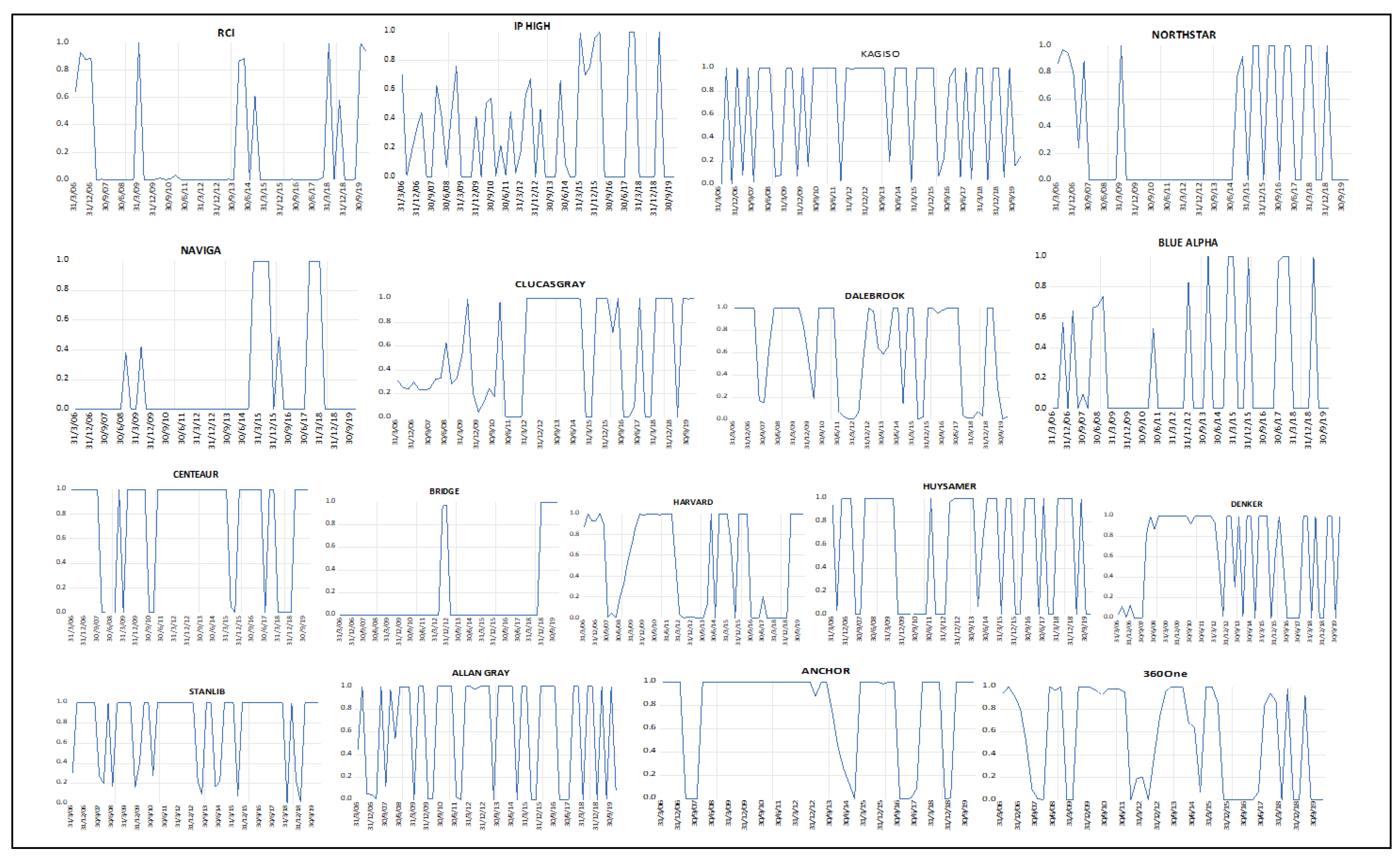
4.4. Smoothed Regime Probabilities

Figure 1 and Figure 2 plot the smoothed probability of regime 1, the bullish state, P[St = 1], fitted to the 33 funds’ performances for the regime switching model specified in Equation 16. The values of the smoothed probability series are typically very close to either zero (regime 2, bearish state) or one (regime 1, bullish) and the smoothed probability series do not frequently switch between the bullish state and the bearish state. The smoothed probability is of interest in economically interpreting the regime switching behavior of the performance of funds and when they occur. From Figure 1, it can be observed that most funds experienced significant volatilities and declines in performance during the period of global financial meltdown, as funds’ performance generally entered a bearish state (regime 2) for a specified period of time.

The performance of funds generally recovered from the bearish state at the beginning of 2009, when they entered a bullish state (regime 1). The presence of bullish performance across funds around 2017/2018 can be explained as flow-driven performance and not as a result of superior trading expertise of fund managers, as investors’ cash allocations to funds increased significantly during this period (Rangongo 2018). This represents a dynamic form of adaptation to changing market conditions by way of wind fall returns on the part of fund managers, which can be explained by the AMH. In general, the performance funds in the sample are highly volatile under changing market conditions. This evidence is closely linked with the position of the extant literature. Turtle and Zhang (2012) employed Markov switching regressions to analyze the time-varying performance of mutual funds. Their evidence suggests that the risk-adjusted performance of mutual funds varies with the dynamics of markets that are dominated by international investments, as they are susceptible to the effects of international market fluctuations. They explained that emerging market funds (South Africa included) exhibit superior performance when the global financial outlook assumes a positive trend relative to returns on investments, implying a significant dependence on foreign inflows. Foreign exchange volatility was identified as a significant determinant of emerging markets funds’ performance. Scholars have explained that during the period of the financial crisis, the level of risk increased, and funds experienced high levels of outflow that caused higher volatility (Ben-David et al. 2012; Manconi et al. 2012). Furthermore, the increased volatility in fund performance of South African funds is linked to capital reallocation from emerging markets to advanced markets during the financial crisis in furtherance with the flight-to-safety hypothesis (Fratzscher 2012). Overall, the inconsistent flow-performance patterns among sampled funds makes it difficult to draw any other conclusion about the performance of mutual funds in South Africa compared to explaining that the dynamics of their performance lack stability. This corresponds with the estimated average regime transition probabilities and the expected durations presented in Table 3 and

Table 4. Regime transition probabilities.

	Regime 1	Regime 2
Regime 1	0.659	0.340
Regime 2	0.314	0.669

Source: Authors’ estimations (2021).

, which shows that a significant percentage of the transition period is spent in the volatile (bearish) condition of the market.

4.5. Regime State Analysis

Regime transition probabilities and expected durations in bullish and bearish conditions are reported in Table 4 and

Table 5. Expected durations.

	Probability	Duration
Regime 1	0.491	4.43
Regime 2	0.509	4.59

Source: Authors’ estimations (2021).

, respectively. Table 4 reports the average transition probabilities between different regimes of the system for the sampled funds. From the table, the average probability of staying in the bullish state (regime 1) is 0.659 while the probability of regime 1 transitioning to regime 2 (bearish state) is 0.340. The probability of staying in the bearish regime (regime 2) is 0.669 and the probability of regime 2 transitioning to regime 1 is 0.314. These results suggest that regime 2 has the highest continuous probability, and hence, is the most stable regime.

Table 5 reports the average expected duration of regime transitions of the estimated MS model. From the table, regime 1, which denotes the bullish condition, is expected to persist for an average of 4.43 quarters while regime 2, denoting the bearish condition, is expected to persist for 4.59 quarters on average, which represents 49.1% and 50.9% of the sample period, respectively. Regime 2 (which is the bearish condition) is the most persistent regime as it accounts for 50.9% of the constant expected duration for the sample period.

5. Conclusions

The purpose of this study was to conduct a non-linear analysis of the determinants of mutual fund performance within a regime switching framework to elicit explanations for the inconsistent flow–performance dynamics in South Africa. As a result, the Markov switching model was employed as a suitable analytical tool to test the effect of fund performance determinants across bullish and bearish conditions of the market. The main findings of the study are presented. First, the predictive power of fund flow over performance is more pronounced in the bearish state of the market than in the bullish state, which is indicative of high investor sensitivity to fund performance in lower periods of the market than in upper periods. Second, similar to the effect of fund flow, other fund-specific variables, namely fund-level fund risk, fund size, and fund age, exert strong deterministic influences on fund performance during market downturns compared to upturns. This finding is linked to the flight-to-liquidity assets and risk-aversion behavior of fund contributors during volatile conditions of the market. Lastly, the study found that the predictive effects of market risk and economic size on fund performance are more evident in bearish market conditions than in bullish conditions. This evidence affirms that the direction of macroeconomic growth and market volatility levels are significant determinants of fund performance. This study contributes to the literature on mutual funds by providing novel perspectives on the effect of fund-specific and systemic factors on fund performance under a regime switching framework in the South African context.

The findings of the study have significant policy implications for fund contributors, fund managers, and economic management frameworks. First, younger funds should remain strategic in their trading activities, as the advantage in fast-paced growth could lead to deteriorations in long-term performance when administrative expenses become excessive as a result of overtrading. In addition, fund managers should remain strategic in market timing to optimize stock-picking choices as increased market volatility affects fund performance. Above all, policymakers should implement policies that create a conducive economic environment as the direction of economic growth and market volatility are linked with fund performance.

This study has recognizable limitations in terms of the variable characteristics and the frequency of data employed in the analysis due to data availability issues. The study mainly focused on measurable fund-level and systemic variables and used quarterly data. Future studies should include variables that capture managerial and investor sentiments as time-varying investor behavior may affect fund performance. Additionally, the use of high-frequency data allows for more data points to enhance the Markov switching analysis.

References

1. Al-Khazali, Osamah, and Ali Mirzaei. 2017. Stock market anomalies, market efficiency and the adaptive market hypothesis: Evidence from Islamic stock indices. Journal of International Financial Markets, Institutions and Money 51: 190–208. [Google Scholar] [CrossRef]
2. Anas, Jacques, Monica Billio, Laurent Ferrara, and Marco Lo Duca. 2007. Business cycle analysis with multivariate markov switching models. Growth and Cycle in the Eurozone, 249–60. Available online: https://core.ac.uk/download/pdf/6234154.pdf (accessed on 20 September 2021).
3. Apau, Richard, Paul-Francois Muzindutsi, and Peter Moores-Pitt. 2021. Mutual fund flow-performance dynamics under different market conditions in South Africa. Investment Management and Financial Innovations 18: 236–49. [Google Scholar] [CrossRef]
4. Areal, Nelson, Maria Céu Cortez, and Florinda Silva. 2013. The conditional performance of US mutual funds over different market regimes: Do different types of ethical screens matter? Financial Markets and Portfolio Management 27: 397–429. [Google Scholar] [CrossRef]
5. Arendse, Jennifer, Chris Muller, and Michael Ward. 2018. The winner takes it all: Outperformance drives subsequent flows in South African Unit Trust Funds. Investment Analysts Journal 47: 1–14. [Google Scholar] [CrossRef] [Green Version]
6. Asisa. 2020. Collective Investments Schemes and Local Funds Statistics. Available online: https://www.asisa.org.za/statistics/collective-investments-schemes/local-fund-statistics/ (accessed on 11 November 2020).
7. Badea, Leonardo, Daniel Ştefan Armeanu, Iulian Panait, and Ştefan Cristian Gherghina. 2019. A Markov Regime Switching Approach towards assessing resilience of Romanian collective investment undertakings. Sustainability 11: 1325. [Google Scholar] [CrossRef] [Green Version]
8. Badrinath, Swaminathan G., and Stefano Gubellini. 2012. Does conditional mutual fund outperformance exist? Managerial Finance 38: 1160–83. [Google Scholar] [CrossRef]
9. Barber, Brad M, Xing Huang, and Terrance Odean. 2016. Which factors matter to investors? Evidence from mutual fund flows. The Review of Financial Studies 29: 2600–42. [Google Scholar] [CrossRef] [Green Version]
10. Ben-David, Itzhak, Francesco Franzoni, and Rabih Moussawi. 2012. Hedge fund stock trading in the financial crisis of 2007–2009. The Review of Financial Studies 25: 1–54. [Google Scholar] [CrossRef] [Green Version]
11. Bertolis, Dino Elias, and Mark Hayes. 2014. An investigation into South African general equity unit trust performance during different economic periods. South African Actuarial Journal 14: 73–99. [Google Scholar] [CrossRef]
12. Bilgili, Faik, Nadide Sevil Halıcı Tülüce, and İbrahim Doğan. 2012. The determinants of FDI in Turkey: A Markov regime-switching approach. Economic Modelling 29: 1161–69. [Google Scholar] [CrossRef]
13. Bojanic, Antonio Nicolás. 2021. A markov-switching model of inflation in Bolivia. Economies 9: 37. [Google Scholar] [CrossRef]
14. Carhart, Mark M. 1997. On persistence in mutual fund performance. The Journal of Finance 52: 57–82. [Google Scholar] [CrossRef]
15. Chevalier, Judith, and Glenn Ellison. 1997. Risk taking by mutual funds as a response to incentives. Journal of Political Economy 105: 1167–200. [Google Scholar] [CrossRef] [Green Version]
16. Chou, Wen-Hsiu, and William George. Hardin. 2014. Performance chasing, fund flows and fund size in real estate mutual funds. The Journal of Real Estate Finance and Economics 49: 379–412. [Google Scholar] [CrossRef]
17. Chung, San-Lin, Chi-Hsiou Hung, and Chung-Ying Yeh. 2014. When does investor sentiment predict stock returns? Journal of Empirical Finance 19: 217–40. [Google Scholar] [CrossRef]
18. Cremers, Martijn, and Antti Petajisto. 2009. How active is your fund manager? A new measure that predicts performance. The Review of Financial Studies 22: 3329–65. [Google Scholar] [CrossRef]
19. Cremers, Martijn, Miguel Almeida Ferreira, Pedro Matos, and Laura Starks. 2016. Indexing and active fund management: International evidence. Journal of Financial Economics 120: 539–60. [Google Scholar] [CrossRef] [Green Version]
20. De la Torre-Torres, Oscar Varela, Evaristo Galeana-Figueroa, and José Álvarez-García. 2020. A test of using markov-switching GARCH models in oil and natural gas trading. Energies 13: 129. [Google Scholar] [CrossRef] [Green Version]
21. Del Guercio, Diane, and Paula A. Tkac. 2002. The determinants of the flow of funds of managed portfolios: Mutual funds vs. pension funds. Journal of Financial and Quantitative Analysis 37: 523–57. [Google Scholar] [CrossRef]
22. Elton, Edwin J., Martin Jay Gruber, and Christopher R. Blake. 1996. The persistence of risk-adjusted mutual fund performance. Journal of Business 69: 133–57. [Google Scholar] [CrossRef] [Green Version]
23. Ferreira, Miguel Almeida, Aneel Keswani, Antonio Freitas Miguel, and Sofia B. Ramos. 2012. The flow-performance relationship around the world. Journal of Banking & Finance 36: 1759–80. [Google Scholar]
24. Ferreira, Miguel Almeida, Aneel Keswani, António Freitas Miguel, and Sofia B. Ramos. 2013. The determinants of mutual fund performance: A cross-country study. Review of Finance 17: 483–525. [Google Scholar] [CrossRef] [Green Version]
25. Franzoni, Francesco, and Martin C. Schmalz. 2017. Fund flows and market states. The Review of Financial Studies 30: 2621–73. [Google Scholar] [CrossRef]
26. Fratzscher, Marcel. 2012. Capital flows, push versus pull factors and the global financial crisis. Journal of International Economics 88: 341–56. [Google Scholar] [CrossRef] [Green Version]
27. Fuerst, Franz, and George Matysiak. 2013. Analysing the performance of nonlisted real estate funds: A panel data analysis. Applied Economics 45: 1777–88. [Google Scholar] [CrossRef]
28. Goetzmann, William N., and Nadav Peles. 1997. Cognitive dissonance and mutual fund investors. Journal of Financial Research 20: 145–58. [Google Scholar] [CrossRef]
29. Granger, Clive William John, and Paul Newbold. 1974. Spurious regressions in econometrics. Journal of Econometrics 2: 111–20. [Google Scholar] [CrossRef] [Green Version]
30. Gray, Stephen F. 1996. Modeling the conditional distribution of interest rates as a regime-switching process. Journal of Financial Economics 42: 27–62. [Google Scholar] [CrossRef]
31. Gueddoudj, Sabbah. 2018. Financial Variables as Predictive Indicators of the Luxembourg GDP Growth. Empirical Economic Review 1: 49–62. [Google Scholar] [CrossRef]
32. Guercio, Diane Del, and Jonathan Reuter. 2014. Mutual fund performance and the incentive to generate alpha. The Journal of Finance 69: 1673–704. [Google Scholar] [CrossRef]
33. Hamilton, James Douglas. 1989. A new approach to the economic analysis of nonstationary time series and the business cycle. Econometrica: Journal of the Econometric Society 57: 357–84. [Google Scholar] [CrossRef]
34. Huang, Feiyu. 2012. An Investigation of the Risk-Adjusted Performance of Canadian REIT Mutual Funds and the Market Timing Skills of fund Managers. Montreal: Concordia University. Available online: https://core.ac.uk/download/pdf/211514431.pdf (accessed on 18 September 2021).
35. Huang, Jennifer Chunyan, Kelsey D. Wei, and Hong Yan. 2012. Investor Learning and Mutual Fund Flows. AFA 2012 Chicago Meetings Paper. Available online: https://ssrn.com/abstract=972780 (accessed on 13 December 2020).
36. Huij, Joop, and Thierry Post. 2011. On the performance of emerging market equity mutual funds. Emerging Markets Review 12: 238–49. [Google Scholar] [CrossRef]
37. Kacperczyk, Marcin, Stijn Van Nieuwerburgh, and Laura Veldkamp. 2016. A rational theory of mutual funds’ attention allocation. Econometrica 84: 571–626. [Google Scholar] [CrossRef] [Green Version]
38. Kim, Chang-Jin. 1994. Dynamic linear models with Markov-switching. Journal of Econometrics 60: 1–22. [Google Scholar] [CrossRef]
39. Kim, Chang-Jin. 2004. Markov-switching models with endogenous explanatory variables. Journal of Econometrics 122: 127–36. [Google Scholar] [CrossRef]
40. Kim, Min Seon. 2019. Changes in Mutual Fund Flows and Managerial Incentives. Available online: https://ssrn.com/abstract=1573051 (accessed on 12 November 2020).
41. Kosowski, Robert. 2011. Do mutual funds perform when it matters most to investors? US mutual fund performance and risk in recessions and expansions. The Quarterly Journal of Finance 1: 607–64. [Google Scholar] [CrossRef]
42. Koy, Ayben. 2017. Regime dynamics of stock markets in the fragile five. Journal of Economic & Management Perspectives 11: 950–58. [Google Scholar]
43. Kunjal, Damien, Faeezah Peerbhai, and Paul-Francois Muzindutsi. 2017. The performance of South African exchange traded funds under changing market conditions. Journal of Asset Management 22: 350–59. [Google Scholar] [CrossRef]
44. Li, Mingsheng, Jing Shi, and Jun Xiao. 2013. Mutual Fund Flow-Performance Relationship under Volatile Market Condition. Paper presented at Asian Finance Association (AsFA) 2013 Conference, Sydney, Australia, January 25. [Google Scholar]
45. Lo, Andrew Wen-Chuan. 2012. Adaptive markets and the new world order (corrected May 2012). Financial Analysts Journal 68: 18–29. [Google Scholar] [CrossRef] [Green Version]
46. Ma, Jason Z., Xiang Deng, Kung-Cheng Ho, and Sang-Bing Tsai. 2018. Regime-switching determinants for spreads of emerging markets sovereign credit default swaps. Sustainability 10: 2730. [Google Scholar] [CrossRef] [Green Version]
47. Manconi, Alberto, Massimo Massa, and Ayako Yasuda. 2012. The role of institutional investors in propagating the crisis of 2007–2008. Journal of Financial Economics 104: 491–518. [Google Scholar] [CrossRef]
48. Nenninger, Steve, and David Rakowski. 2014. Time-varying flow-performance sensitivity and investor sophistication. Journal of Asset Management 15: 333–45. [Google Scholar] [CrossRef]
49. Obalade, Adefemi Alamu, and Muzindutsi Paul-Francois. 2018a. Are there Cycles of Efficiency and Inefficiency? Adaptive Market Hypothesis in Three African Stock Markets. Frontiers in Finance and Economics 15: 185–202. [Google Scholar]
50. Obalade, Adefemi Alamu, and Muzindutsi P.F. 2018b. Return predictability and market conditions: Evidence from Nigerian, South African and Mauritian stock markets. African Journal of Business and Economic Research 13: 7–23. [Google Scholar] [CrossRef]
51. Papadimitriou, Dimitris, Konstantinos Tokis, and Georgios Vichos. 2020. The Effect of Market Conditions and Career Concerns in the Fund Industry. Available online: https://ssrn.com/abstract=3658288 (accessed on 10 June 2021).
52. Pástor, Ľuboš, Robert F. Stambaugh, and Lucian A. Taylor. 2015. Scale and skill in active management. Journal of Financial Economics 116: 23–45. [Google Scholar] [CrossRef]
53. Pastpipatkul, Pathairat, Petchaluck Boonyakunakorn, and Kanyaphon Phetsakda. 2020. The impact of Thailand’s openness on bilateral trade between Thailand and Japan: Copula-based markov switching seemingly unrelated regression Model. Economies 8: 9. [Google Scholar] [CrossRef] [Green Version]
54. Popescu, Marius, and Zhaojin Xu. 2017. Market states and mutual fund risk shifting. Managerial Finance 43: 828–38. [Google Scholar] [CrossRef]
55. Qian, Meifen, Chongbo Xu, and Bin Yu. 2014. Performance manipulation and fund flow: Evidence from China. Emerging Markets Finance and Trade 50: 221–39. [Google Scholar] [CrossRef]
56. Rangongo, Timothy. 2018. A fund with inflation-beating growth-fund in focus: Marriott divided growth fund. Finweek 2018: 14. [Google Scholar]
57. Rao, Zia-Ur-Rehman, and Muhammad Zubair Tauni. 2016. Fund Performance and fund flow. Case of China. Journal of Academic Research in Economics 8: 146–56. [Google Scholar]
58. Rohleder, Martin, Dominik Schulte, and Marco Wilkens. 2017. Management of flow risk in mutual funds. Review of Quantitative Finance and Accounting 48: 31–56. [Google Scholar] [CrossRef]
59. Rupande, Lorraine, Hilary Tinotenda Muguto, and Paul-Francois Muzindutsi. 2019. Investor sentiment and stock return volatility: Evidence from the Johannesburg Stock Exchange. Cogent Economics & Finance 7: 1600233. [Google Scholar]
60. S&P. 2019. SPIVA South Africa Year End 2018 Score Card. Available online: https://www.spglobal.com/spdji/en/doc-uments/spiva/spiva-south-africa-year-end-2018.pdf (accessed on 12 November 2019).
61. Sapp, Travis, and Ashish Tiwari. 2004. Does stock return momentum explain the “smart money” effect? The Journal of Finance 59: 2605–22. [Google Scholar] [CrossRef]
62. Schmidt, Amand Floriaan, and Chris Finan. 2018. Linear regression and the normality assumption. Journal of Clinical Epidemiology 98: 146–51. [Google Scholar] [CrossRef] [PubMed] [Green Version]
63. Sirri, Erik R., and Peter Tufano. 1998. Costly search and mutual fund flows. The Journal of Finance 53: 1589–622. [Google Scholar] [CrossRef]
64. Stafylas, Dimitrios, and Athanasios Andrikopoulous. 2019. Determinants of hedge fund performance during ‘good’and ‘bad’economic periods. Research in International Business and Finance 52: 101130. [Google Scholar] [CrossRef]
65. Tan, Ömer Faruk. 2015. Mutual Fund Performance: Evidence from South Africa. EMAJ: Emerging Markets Journal 5: 49–57. [Google Scholar] [CrossRef] [Green Version]
66. Tsagris, Michail, and Nikolaos Pandis. 2021. Normality test: Is it really necessary? American Journal of Orthodontics and Dentofacial Orthopedics 159: 548–49. [Google Scholar] [CrossRef] [PubMed]
67. Turtle, Harry J., and Chengping Zhang. 2012. Time-varying performance of international mutual funds. Journal of Empirical Finance 19: 334–48. [Google Scholar] [CrossRef] [Green Version]
68. Urquhart, Andrew, and Frank McGroarty. 2014. Calendar effects, market conditions and the Adaptive Market Hypothesis: Evidence from long-run US data. International Review of Financial Analysis 35: 154–66. [Google Scholar] [CrossRef]
69. Urquhart, Andrew, and Frank McGroarty. 2016. Are stock markets really efficient? Evidence of the adaptive market hypothesis. International Review of Financial Analysis 47: 39–49. [Google Scholar] [CrossRef] [Green Version]
70. Xiao, Jun, Mingsheng Li, and Jing Shi. 2014. Volatile market condition and investor clientele effects on mutual fund flow performance relationship. Pacific-Basin Finance Journal 29: 310–34. [Google Scholar]
71. Yu, Shun-Zheng, and Hisashi Kobayashi. 2006. Practical implementation of an efficient forward-backward algorithm for an explicit-duration hidden Markov model. IEEE Transactions on Signal Processing 54: 1947–51. [Google Scholar]
72. Ziphethe-Makola, Sandiswa Masande. 2017. Relationship between AUM and Alpha in SA Mutual Funds. Master’s thesis, University of Cape Town, Cape Town, South Africa. [Google Scholar]
Figure 1. Smoothed probability of regime 1 (bullish state) for the Markov switching model.
Economies 09 00161 g001
Figure 2. Smoothed probability of regime 1 (bullish state) for the Markov switching model.
Economies 09 00161 g002