Abstract
Global liquidity shortage as well as the availability on the market of overpriced assets and derivatives led to the situation where the global economy depends primarily on liquidity, becoming prone to chain-consistent world crises. Only for the last 15 years, the world has witnessed a continuous series of crises. Therefore, the study of the processes and phenomena of crisis is one of the most important scientific and practical tasks. The aim of this work consisted in the development of methods and models for the early detection of crises in the economy. The significance of the work is to develop an econometric model and tools for detection of crisis.
1. Introduction
The global shortage of liquidity and presence of overvalued, low-liquid assets and derivatives on the market have led to a situation where the world economy, being primarily dependent on the amount of liquidity, became subject to successive world crises. Over the past 15 years alone, the world has experienced a continuous series of crises (). Today, market trends, as well as crises market states and bankruptcies, are the fundamental factors affecting the development of the world economy (). Therefore, the study of crisis processes and phenomena in the economy is one of the most important scientific and practical tasks (; ). Crisis is not an instantaneous and unexpected process, but, on the contrary, an inherent property of the economic system, and it has a certain rate of development. The beginning of the crisis is impossible to predict. But if the crisis has already started, one can define (register) the initial phase of the crisis. Hence, its further development can be predicted at the next stage (). The term «financial crisis» is widely used in situations where financial assets suddenly lose a large part of their nominal value. In the late 19th and early 20th centuries, a large part of financial crises was associated with bank panic. Stock market crashes and collapses of financial bubbles, currency crises, and sovereign defaults also inherently impacted financial crises. Many economists have proposed the theory of development and the prevention of financial crises.
The authors (, ) located the hidden patterns underlying the financial crisis using the concept of recurrence plots to study the stock market. The authors claimed that their method is efficient in the detection of financial bubbles.
The authors () analyzed the annual signals on the US stock market, transformed the signals into a Fourier series, and concluded that, as a global financial crisis approaches, low-frequency components increase more sharply than high-frequency components. The authors () employed the log-periodic power law (LPPL) to analyze the financial crisis. They proposed the concept of a mechanism behind the heavy withdrawal of funds from banks (bank runs) and made conclusions of banks’ refinancing options. The authors () examined the effect of COVID-19 and negative and positive news (shocks) on the volatility of Australian stock returns. The authors () showed that interest, credit, and currency channels of the monetary policy transmission mechanism can be used to overcome the trust crisis in the financial sector.
Despite a number of successful works in this field, scientists have not been able to come to a consensus on how to identify and manage crises.
The purpose of this study was to investigate the crisis phenomena and processes in the asset market and to build an econometric model of crisis. The article proposes the author’s concept of the crisis process understood as a sequence of imbalance states and stabilization of the ratio of market supply and demand indicators, which has pronounced phases of growth, plateau, and decline, and intermediate states, primary and secondary reversals, characterized by the presence of bifurcation points or crisis equilibriums. In contrast to the classical approach, the author considers economic crisis not as a non-recurrent state, for example, the bifurcation point in the equilibrium model of the crisis of Paul () or the point of market saturation in the theory of Karl ( (), but as an ongoing process. The classification of its main phases based on statistical indicators was proposed. A method of early detection of the initial crisis phase as a state of statistical unpredictability, resulting in the indicator going beyond statistically valid bounds, was developed.
The research includes several sections. In the first section, we study higher-order moments that can be used to detect outliers in financial time series. The second section provides an overview of existing stock indicators and an analysis of the properties of time series. Based on the identified patterns in the time series, a crisis indicator is developed that captures the crisis at an early stage. The study ends with a section in which an econometric model of the crisis is proposed, providing a possibility to predict the ending moment of the asset crisis.
2. Literature Review
Let us consider the history of the occurrence of financial crises.
Figure 1 shows a historical summary of global crises.
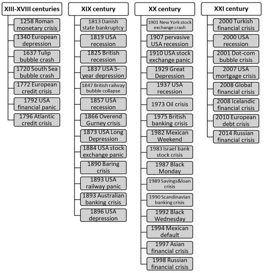
Figure 1.
Classification of global crises.
Among the most prominent economists who made contributions in the research of economic crises were Karl (), who believed that they were inevitable, and John Maynard (), whose theory suggested that a crisis-free economy was possible. However, Israel () questioned the objectivity of both Marx’s and Keynes’s models. Later on, Paul () proposed a crisis model that came to be regarded as conventional.
Today, there are three well-established concepts of the crisis, namely, Austrian, Marxist, and Keynesian.
The Austrian business cycle theory (ABCT), developed by the Austrian School of economics, explains the principle according to which economic crises (cycles) occur. It views business crises (cycles) as the consequence of excessive growth in bank credit due to artificially low interest rates set by a central bank or fractional-reserve banks. The Austrian business cycle theory originated in the work of Austrian School economists L. von Mises and F. ().
Marxist theory. After J. S. de Sismondi (1773–1842) put forward the first theory of crisis, criticizing the premise of the existence of an equilibrium between supply and demand, economists focused on the study of periods of depression in the world economy that occur every 20 to 50 years (which are often referred to as economic cycles in the literature). The theory of economic crisis was developed by Karl ().
The effectiveness of this theory depends on two main factors: first, the amount of taxes imposed on profits by the state and returned to the population in the form of social security, family benefits, health care, and education; and second, the ratio of the number of workers employed to the number of investors/business owners in society. Additional capital expenditures are required to enter modern markets, such as air transportation, military industry, or chemical production markets. Entering these markets is extremely difficult for new firms, so business is concentrated in the hands of fewer and fewer companies.
Keynesian theory. John Maynard () developed a theory applicable to a closed economy, which was later refined by Hyman (). The latter provided a theoretical justification for the hypothesis that financial instability is a typical feature of any capitalist economy. High instability leads to an increased risk of a financial crisis.
In the aspect of Keynesian theory, in 1999 Krugman proposed the crisis model, which is currently considered the most developed ().
Many modern scientists are engaged in the study of crises. For example, Korobeinikov in his work () describes the crisis model as a catastrophic epidemic of bankruptcies. He considers the economy as a population of interacting economic agents of a certain size N. The author divides the population into two groups, namely, the «healthy» subpopulation of size x(t) and the “activated” subpopulation of size y(t). The members of the second group have financial difficulties or are unable to fulfil their financial obligations. It is assumed that the activated agents can activate the healthy agents, with which they are in a business relationship, but to be activated, an average healthy agent has to come into contact with α activated agents. After presenting the process of activating as , it is concluded that the activation occurs at the rate , where is the activation rate coefficient.
Another mathematical model of crisis is provided by P. (), as they distinguish three market conditions—growth, decline, and crisis—as separate qualitative categories and focus on banking crisis identification.
Since the rise of volatility is one of the key indicators of the onset of a crisis, let us consider a number of contemporary studies that are relevant on a practical level and empirically justify the relationship between volatility and crisis.
One of the modern case studies of crisis published by Phornchanok Cumperayot and Roy Kouwenberg () employs a multivariate extreme value approach to create an early warning system for currency crises.
() conducted an analysis that revealed the relationship between increased volatility and the onset of a banking crisis.
The next research focuses on the volatility spillover effect and financial contagion. D. () empirically proved an increase in the correlation coefficient between volatility indices in various markets during the crisis period and linked this to behavioral factors.
Stephen () demonstrated that, under the condition of no-arbitrage, the return volatility is directly related to the rate of information flows. The consequence of this conclusion is that a sharp change in the level of volatility of a particular market can lead to a change in the level of volatility of other related markets.
The next section is devoted to the spread of volatility in international financial markets. Vasyl () developed an approach that takes into account the presence of two potential channels of volatility spillover, namely, the «volatility transmission» from one market to others through its variance and covariance. The authors assumed that there is a spillover channel through covariance due to the existence of empirical evidence that sharp changes in variance lead to an increase in the correlation coefficient in the world market.
Shaen () conducted a study to determine how the volatility is affected by the news background containing sell and buy recommendations for Greek financial institutions during times of growth, decline, and crisis in the Greek equity market.
T. () conducted an empirical study of stock returns and volatility spillover, and the effect of borrowing from stock markets of larger developed countries (Germany, Great Britain, and the USA) to support stock markets of smaller EU member states (Italy, Ireland, Greece, Spain, and Portugal) in the period from 2002 to 2014. The GJR-GARCH model was used to explore the impact of the financial crisis on the spillover effect.
M. Sergio et al. () analyzed the occurrence of bubbles and the associated volatility.
Summing up, we can conclude that an increase in the volatility indicator is an important warning signal of the crisis.
3. Modeling of Crisis Processes Based on Moments of Higher Orders
When modeling crisis processes, the moments of higher orders play an important role.
A moment is a point estimate of the central trend of some characteristic of a random variable.
The raw moment of the k-th order of a random variable X is the mathematical expectation of the k-th degree of this quantity:
The absolute raw moment of the k-th order is the mathematical expectation of the k-th degree of the modulus of a random variable.
The raw moments of even orders are absolute.
The raw moment of the 0-th order is always equal to one.
The raw moments are not reduced values; the reduced raw moment corresponds to taking the root of degree i.
The absolute reduced raw moment of the k-th order is:
The central moment of the k-th order of a random variable X is the mathematical expectation of the k-th degree of deviation of the random variable X from its mathematical expectation:
The absolute central moment of the k-th order is the mathematical expectation of the k-th degree of the modulus of deviation of a random variable X from its mathematical expectation.
The central moments of even orders are absolute.
The central moment of the 0-th order is always equal to one.
The central moments are not reduced values; the reduced raw moment corresponds to taking the root of degree k.
The k-th moment of a random variable of X is equal to . The first two moments are useful because they provide the mean and variance , which are important indicators of the distribution. The third and fourth moments show the skewness of the distribution in the behavior of the tails or extreme values.
Types of moments. Let X be a random variable with the mean µ and the variance. For any positive integer k, the k-th moment of X is equal to , the n-th central moment is equal to , and the k-th standardized moment is equal to .
Let us define the skewness, which is based on the third moment. Skewness is defined as the third standardized moment.
- If the distribution is symmetric with respect to the mathematical expectation, then the coefficient of skewness is .
- If , then the distribution has a right-sided skewness.
- If , then the distribution has a left-sided skewness.
Kurtosis of the random variable X with the mean value µ and the variance σ2 has the form:
Curves that are more peaked than normal have a positive kurtosis, and curves that are more flat-topped have a negative kurtosis.
If , then the distribution is thin pointed.
If , then it is a broad, flat distribution.
High-order moments are moments outside of the fourth-order moments.
When analyzing time series, three types of raw moments are used, which differ in time characteristics.
The total moment is the moment of the entire time series. The total moment is necessary for the economy to conduct research in the medium and long term and not only in the short term.
The fixed moment is a moment corresponding to a certain time interval. The fixed moment is used to analyze the state of the market: stagnation, growth, or crisis.
The cumulative moment is the total moment calculated sequentially for each time period.
Moments of even orders reflect unsigned (scalar) characteristics of the time series. Moments of odd orders reflect the directional (vector) characteristics of the time series.
The higher the order of the moment, the more it reflects the characteristics of outliers and deviations. Higher-order raw moments are usually used to identify areas that are uncharacteristic of the series as a whole (for example, outliers or crises) (see Figure 2 and Figure 3).
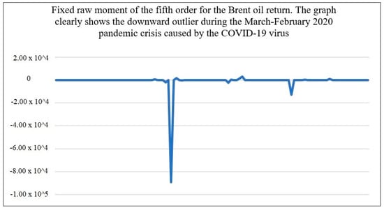
Figure 2.
Fixed raw moment of the fifth order for the Brent oil return.
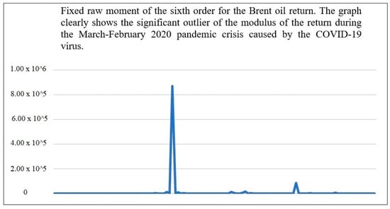
Figure 3.
Fixed raw moment of the sixth order for the Brent oil return.
The higher the moment, the stronger the extreme value is visible.
4. Development of an Indicator for Crisis Detection
According to the amount of data used, all indicators are divided into three types:
- Instantaneous (using only current data);
- Moving averages (using, in addition to the current data, previous data for a certain period);
- Cumulative (using all the data from the beginning of the time series).
According to the processing of the data used, indicators can be divided into two types:
- Direct (not using intermediate calculations);
- Indirect (using intermediate calculations).
Based on the time series of the dollar exchange rate, we will consider three direct indicators belonging to different types.
- An instantaneous indicator that determines the crossing of a certain bound. Figure 4 shows a graph of the instantaneous indicator.
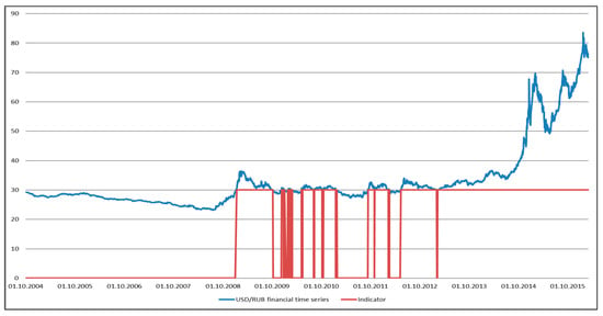 Figure 4. Graph of crossing of the 30 threshold.
 - A moving indicator that determines the 30-day average (moving average) (see Figure 5).
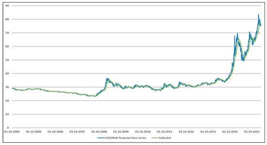 Figure 5. The moving indicator that determines the average for 30 days.
 - Cumulative indicator that calculates the achieved mathematical expectation (see Figure 6).
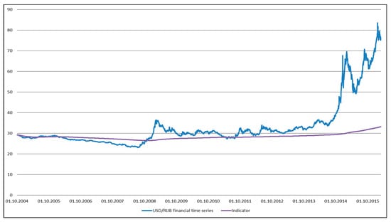 Figure 6. The cumulative indicator that calculates the achieved mathematical expectation.
When analyzing time series, three methods of normalization (it is generally accepted to normalize to one) and their combinations are used.
- Scaling by the maximum of the series is used in cases when the series is completed and there will be no new data.
- Scaling by the current maximum reached is used when the next data are expected to arrive.
- Nonlinear reversible compression is used to improve the statistics of data with a large number of outliers.
Based on the time series of the dollar exchange rate, we will consider three normalization methods and their combinations.
Figure 7 shows graphs of the normalization methods.
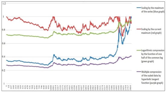
Figure 7.
Graphs of various normalization methods.
The main property of the central tendency measure is its robustness (resistance to outliers), sometimes characterized as plausibility.
Depending on the type of statistical scale, there are four types of weakly robust measures of central tendency, shown in Figure 8.
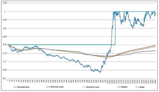
Figure 8.
Graphs of central tendency measures.
5. Variability
Variability is a measure of central tendency (singular number) that characterizes the deviations of the sample values from their overall measure of central tendency (mean value).
The main values expressing the variability depend not only on the expressed value but also on the time period during which it is estimated.
In econometrics, the eight main measures of variability are most commonly used. All of them have different robustness, sensitivity, and purpose depending on the scale. Measures of variability include:
- Mean absolute deviation (MAD) is the average of the modulus of deviations of the series values from its mathematical expectation.
- Variance is the mathematical expectation of the squares of absolute deviations.
- Mean square deviation (standard deviation) is the square root of the variance.
- Scedasticity (relative variability) is the ratio of the modulus of deviations to the mathematical expectation.
- Mean cubic deviation is used to identify the trend of growth/decline hidden by white noise. An example is the cubic root of the mathematical expectation of cubes of absolute deviations.
- Mean progressive deviation is used to identify the trend of hidden growth.
- Mean structural deviation is used in the frequency analysis of econometric data.
- Volatility is a measure of the variability of a time series expressed with reference to a time scale. The ratio of the standard deviation to the root of the time period expressed in years.
Figure 9 shows graphically the measures of variability.
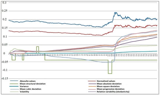
Figure 9.
Graphs of variability measures.
Consider the assumption that the tripled instantaneous variability cannot exceed the variability accumulated over a long period. Figure 10 shows examples of simple indicators.
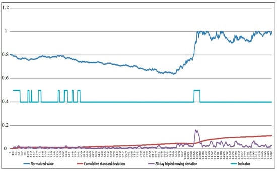
Figure 10.
Types of indicators.
We will introduce the concept of the asset crisis, which is the movement in the value of the asset inconsistent with the standard Black–Scholes model ().
The key idea behind this model involves stationarity and normality of the cumulative variability of the time series representing the Gaussian (normally distributed) noise. This idea is the basis of most autoregressive forecasting mathematical models in economics and equity analytics (e.g., ARMA). In the event of a crisis, the behaviors of the variability assumed by the model are violated (for example, the three-sigma rule). To determine the crisis it is necessary to compare the long-term cumulative variability with the current variability of the moving sample. According to the model implying the normality of the deviations of the series, its triple instantaneous variability cannot exceed the long-term cumulative variability.
We will offer a method of constructing a crisis indicator that defines the crisis at an early stage. The method of creating a crisis indicator is based on the key empirical properties of volatility. Relying on the three-sigma rule (), stating that practically all of the values are normally distributed random variables lying within the interval, [M − 3σ; M + 3σ] asked to assess the crisis as the output volatility index for statistically predictable limits. In this case, it means that the distribution of the time-series volatility is close to normal. Thus, the beginning of the crisis is changing the basic indicator (asset volatility) beyond the predictable probability (statistically in 99.7%). Therefore, as a crisis indicator, the integrative assessment of triple error volatility can be used, the benchmark for which is the current value of volatility where means the volatility of fluctuations ().
When using this indicator we should keep in mind that at the time of the release volatility index outside , the time series of the volatility index ceases to be stationary in the wide sense and does not revert to the state of general stationarity until the end of the crisis. Therefore, according to the general principles of reduction of heteroscedasticity, it must consider the crisis as an “area of incompetence stationary model” and exclude it from further calculations of the volatility index.
The main empirical properties of volatility are the tendency to clustering, long memory (autocorrelation), and high correlation with trading volume (). It is on these properties that the classic predictive models Garch, Arch, and similar are based, suggesting that the volatility is a stochastic process note Chand, Sohail, Shahid Kamal, and Imran Ali in their study process (). These models use standard Gaussian or Student distribution. In cases where the volatility goes beyond the predictability in the three sigmas of the used models, the standard methods of forecasting volatility stop working. It does not allow economists to assess adequately the risks and usually leads to the stock panic, which is the trigger of the crisis of the traded asset.
Let us develop an indicator that identifies a crisis at an early stage (). The initial phase of the crisis development will be defined by the Formula (31):
where is crisis intensity, is indicator sensitivity coefficient, is volatility deviation, and is volatility (mean-square deviation).
Figure 11 and Figure 12 provide an analysis of the crisis indicator operation based on the example of the time series of USD/RUB.
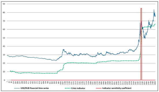
Figure 11.
The crisis indicator. The coefficient of sensitivity of the indicator is 1.
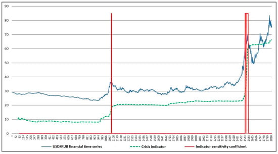
Figure 12.
The crisis indicator. The coefficient of sensitivity of the indicator is 3.
6. Model of Crisis
Let us define a crisis as a situation of change in the asset value that exceeds the statistically permissible limits.
We identify the beginning of the crisis as the process of transition of the volatility indicator into a non-stationary state followed by its return to the state of stationarity in the wide sense.
To build an econometric model of the crisis, 149 assets were selected from the general population of assets of the Moscow Exchange that met the following conditions: The asset had at least one crisis period; it had been traded on the Moscow Exchange for at least 5 years; price data were available for the entire trading period. The total number of detected and analyzed crisis periods was 708. Figure 13 shows the analysis of the crisis variability.
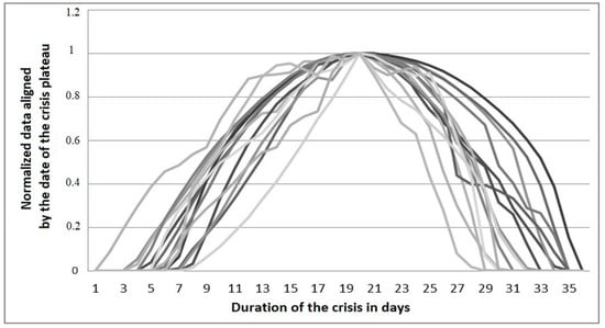
Figure 13.
Analysis of the crisis variability. Duration of crises in days.
A trial approximation of the crisis values of volatility was carried out using simple functions. As approximating functions, we tried the following:
- Power function: R = 0.942
- Sixth-order polynomial: R = 0.994
- Trigonometric functions: R = 0.997
As a result, to describe the mathematical model of the asset crisis it was decided to use a function of the form: ; and to determine the phases of the crisis, we used its derivatives of the first and second order.
The econometric model of the crisis development may include six stages characterized by the first- and second-order derivatives of the approximating function of the standard deviation of volatility . Table 1 shows the stages of the crisis development.

Table 1.
Stages of the crisis development.
Figure 14 shows the main phases of development and decay of a crisis process.
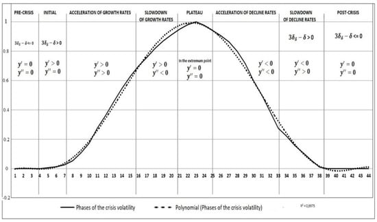
Figure 14.
Phases of the crisis development.
A mathematical model (Equation (1)) was created that allows us not only to determine the current phase of the crisis, but also after passing the plateau, to predict its ending moment with sufficient accuracy.
Figure 15 shows an econometric model of the crisis.
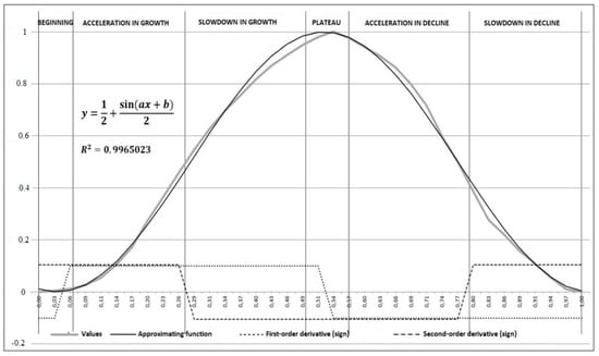
Figure 15.
Model of the crisis.
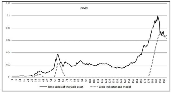
Figure 16.
Identification of the crisis based on the Gold price time series.
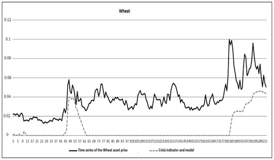
Figure 17.
Identification of the crisis based on the Wheat price time series.
It should be noted that the developed model of the crisis demonstrated good efficiency and applicability only in the asset market. Global crises cannot be analyzed based on an econometric model. However, they are well described by network models, for example, the Korobeinikov model ().
In the course of further research, it is possible to ground this model using statistical criteria and improve its accuracy. It is necessary to expand the scope of this model and test it not only on the Russian financial market but also on foreign asset markets.
7. Conclusions
The analysis of existing crisis models makes evident their shortcomings, specifically, low-level abstract models demonstrate excessive concretization expressed predominantly in the consideration of a crisis in the context of the beginning of the asset value collapse as a fait accompli. However, the specific changes proposed by the authors of the models as the attribute of a crisis situation expressed in absolute numerical terms do not in the least guarantee the actual presence of crisis and are not well substantiated, either statistically or mathematically. At the same time, the point estimation bankruptcy = crisis, no bankruptcy = no crisis, used in the model of A. () without due mathematical or econometric justification also makes this technique as inapplicable in practice. The developed econometric model of the crisis is mathematically justified and is easily applicable in practice.
With the developed model, economists get a tool that can be used to detect the crisis at an early stage and take appropriate measures to mitigate it. Making the right decision timely often becomes a saving option for a soft passage of the crisis. According to I. (), it is impossible to avoid a crisis, but its consequences can be mitigated. As a practical example, we can think of an analysis of the situation at the height of the 2008 crisis, when a timely decision to launch a quantitative easing program in the United States helped save the banking system of this country, thereby mitigating the consequences of the crisis.
Funding
This research received no external funding.
Institutional Review Board Statement
Not applicable.
Informed Consent Statement
The authors declare no conflict of interest.
Data Availability Statement
The website finam.ru was used to import the data.
Conflicts of Interest
The author declares no conflict of interest.
References
- Addo, Peter Martey, Monica Billio, and Dominique Guegan. 2013. Nonlinear dynamics and recurrence plots for detecting financial crisis. The North American Journal of Economics and Finance 26: 416–35. [Google Scholar] [CrossRef] [Green Version]
- Addo, Peter Martey, Monica Billio, and Dominique Guégan. 2014. Nonlinear dynamics and wavelets for business cycle analysis. In Wavelet Applications in Economics and Finance. Cham: Springer, pp. 73–100. [Google Scholar]
- Brychko, Maryna, Yuriy Bilan, Serhiy Lyeonov, and Grzegorz Mentel. 2021. Trust crisis in the financial sector and macroeconomic stability: A structural equation modelling approach. Economic Research-Ekonomska Istraživanja 34: 828–55. [Google Scholar] [CrossRef]
- Cartea, Álvaro, and Dimitrios Karyampas. 2011. Volatility and covariation of financial assets: A high-frequency analysis. Journal of Banking & Finance 35: 3319–34. [Google Scholar] [CrossRef] [Green Version]
- Chand, Sohail, Shahid Kamal, and Imran Ali. 2012. Modeling and volatility analysis of share prices using ARCH and GARCH models. World Applied Sciences Journal 19: 77–82. [Google Scholar] [CrossRef]
- Choudhry, Taufiq, Fotios I. Papadimitriou, and Sarosh Shabi. 2016. Stock market volatility and business cycle: Evidence from linear and nonlinear causality tests. Journal of Banking & Finance 66: 89–101. [Google Scholar] [CrossRef] [Green Version]
- Corbet, Shaen, Michael Dowling, and Mark Cummins. 2015. Analyst recommendations and volatility in a rising, falling, and crisis equity market. Finance Research Letters 15: 187–94. [Google Scholar] [CrossRef]
- Cumperayot, Phornchanok, and Roy Kouwenberg. 2013. Early warning systems for currency crises: A multivariate extreme value approach. Journal of International Money and Finance 36: 151–71. [Google Scholar] [CrossRef]
- Fariborz, Moshiriana, and Qiongbing Wu. 2009. Banking industry volatility and banking crises. Journal of International Financial Markets, Institutions and Money 19: 351–70. [Google Scholar] [CrossRef]
- García-Carranco, Sergio M., Juan Bory-Reyes, and Alexander S. Balankin. 2016. The crude oil price bubbling and universal scaling dynamics of price volatility. Physica A: Statistical Mechanics and Its Applications 452: 60–68. [Google Scholar] [CrossRef]
- Gataullin, Timur M., Sergey T. Gataullin, and Ksenia V. Ivanova. 2020. Modeling an Electronic Auction. In Institute of Scientific Communications Conference. Cham: Springer, pp. 1108–17. [Google Scholar]
- Golosnoy, Vasyl, Bastian Gribisch, and Roman Liesenfeld. 2015. Intra-daily volatility spillovers in international stock markets. Journal of International Money and Finance 53: 95–114. [Google Scholar] [CrossRef]
- Hayek, Friedrich August. 2014. The Fortunes of Liberalism: Essays on Austrian Economics and the Ideal of Freedom. Ludwig von Mises (1881–1973). London: Routledge, pp. 138–71. ISBN 9780415035163. First published 1992. [Google Scholar]
- Iqbal, Najam, Muhammad Saqib Manzoor, and Muhammad Ishaq Bhatti. 2021. Asymmetry and Leverage with News Impact Curve Perspective in Australian Stock Returns’ Volatility during COVID-19. Journal of Risk and Financial Management 14: 314. [Google Scholar] [CrossRef]
- Ivanyuk, Vera. 2019. Phase model of asset crises identification. Scientific Publications of the State University of Novi Pazar Series A: Applied Mathematics, Informatics and Mechanics 11: 55–60. [Google Scholar] [CrossRef]
- Ivanyuk, Vera. 2021. Formulating the Concept of an Investment Strategy Adaptable to Changes in the Market Situation. Economies 9: 95. [Google Scholar] [CrossRef]
- Jun, Doobae, Changmo Ahn, Jinsu Kim, and Gwangil Kim. 2019. Signal analysis of global financial crises using Fourier series. Physica A: Statistical Mechanics and its Applications 526: 121015. [Google Scholar] [CrossRef]
- Jutasompakorn, Pearpilai, Robert Brooks, Christine Brown, and Sirimon Treepongkaruna. 2014. Banking crises: Identifying dates and determinants. Journal of International Financial Markets, Institutions and Money 32: 150–66. [Google Scholar] [CrossRef]
- Kenourgios, Dimitri. 2014. On financial contagion and implied market volatility. International Review of Financial Analysis 34: 21–30. [Google Scholar] [CrossRef]
- Keynes, John Maynard. 2012. The Collected Writings of John Maynard Keynes. Edited by Donald E. Moggridge and Elizabeth S. Johnson. London: Royal Economic Society, vol. 1. First published 1978. [Google Scholar] [CrossRef]
- Kirzner, Israel M., ed. 1986. Subjectivism, Intelligibility and Economic Understanding: Essays in Honor of Ludwig M. Lachmann on His Eightieth Birthday. New York: New York University Press. [Google Scholar]
- Korobeinikov, Andrei. 2009. Financial crisis: An attempt of mathematical modelling. Applied Mathematics Letters 22: 1882–86. [Google Scholar] [CrossRef] [Green Version]
- Krugman, Paul R. 1999. The Return of Depression Economics. New York: W. W. Norton & Co Inc., pp. 70–77. [Google Scholar]
- MacBeth, James D., and Larry J. Merville. 1979. An empirical examination of the Black-Scholes call option pricing model. The Journal of Finance 34: 1173–86. [Google Scholar] [CrossRef]
- Marx, Karl Heinrich. 2007. Capital: A Critique of Political Economy. Edited by Bruce B. Lawrence and Aisha Karim. Durham: Duke University Press, pp. 63–77. First published 1867. [Google Scholar] [CrossRef]
- Mikhaylov, Alexey. 2020. Cryptocurrency Market Analysis from the Open Innovation Perspective. Journal of Open Innovation: Technology, Market, and Complexity 6: 197. [Google Scholar] [CrossRef]
- Minsky, Hyman P. 2008. Stabilizing an Unstable Economy. Princeton: McGraw-Hill Education. First published 1986. [Google Scholar]
- Mohti, Wahbeeah, Andreia Dionísio, Paulo Ferreira, and Isabel Vieira. 2019. Contagion of the subprime financial crisis on frontier stock markets: A copula analysis. Economies 7: 15. [Google Scholar] [CrossRef] [Green Version]
- Prigogine, Ilya. 1978. Time, structure, and fluctuations. Science 201: 777–85. [Google Scholar] [CrossRef] [PubMed] [Green Version]
- Pukelsheim, Friedrich. 1994. The three sigma rule. The American Statistician 48: 88–91. [Google Scholar] [CrossRef]
- Ross, Stephen A. 1976. The arbitrage theory of the capital asset pricing model. Journal of Economic Theory 13: 341–60. [Google Scholar] [CrossRef]
- Soloviev, Vladimir, Nikita Titov, and Elena Smirnova. 2020. Coking Coal Railway Transportation Forecasting Using Ensembles of ElasticNet, LightGBM, and Facebook Prophet. In International Conference on Machine Learning, Optimization, and Data Science. Cham: Springer, pp. 181–90. [Google Scholar] [CrossRef]
- Wosnitza, Jan Henrik, and Cornelia Denz. 2013. Liquidity crisis detection: An application of log-periodic power law structures to default prediction. Physica A: Statistical Mechanics and Its Applications 392: 3666–81. [Google Scholar] [CrossRef]
- Zhang, Yang, Juanita Trusty, Tatiana Goroshnikova, Louise Kelly, Kwok K. Kwong, Stephen J. J. McGuire, Juan Perusquia, Veena P. Prabhu, Minghao Shen, and Robert Tang. 2021. Millennial social entrepreneurial intent and social entrepreneurial self-efficacy: A comparative entrepreneurship study. Social Enterprise Journal 17: 20–43. [Google Scholar] [CrossRef]
Publisher’s Note: MDPI stays neutral with regard to jurisdictional claims in published maps and institutional affiliations. |
© 2021 by the author. Licensee MDPI, Basel, Switzerland. This article is an open access article distributed under the terms and conditions of the Creative Commons Attribution (CC BY) license (https://creativecommons.org/licenses/by/4.0/).