Convergence and Heterogeneity in Euro Based Economies: Stability and Dynamics

Abstract

Cluster analysis is used to explore the performance of key macroeconomic variables in European countries that share the euro, from the inception of the currency in 2002 through to 2013. An original applied statistical approach searches for a pattern synthesis across a matrix of macroeconomic data to examine if there is evidence for country clusters and whether there is convergence of the cluster patterns over time. A number of different clusters appear and these change over time as the economies of the member states dynamically interact. This includes some new countries joining the currency during the period of examination. As found in previous research, Southern European countries tend to remain separate from other countries. The new methods used, however, add to an understanding of some differences between Southern European countries, in addition to replicating their broad similarities. Hypotheses are formed about the country clusters existing in 2002, 2006 and 2013, at key points in time of the euro integration process. These hypotheses are tested using the rigour of a bivariate analysis and the multivariate method of Qualitative Comparative Analysis (QCA). The results confirm the hypotheses of cluster memberships in all three periods. The confirmation analysis provides evidence about which variables are most influencing cluster memberships at each time point. In 2002 and 2006, differences between countries are influenced by their different Harmonised Index of Consumer Prices (HICP) and labour productivity scores. In 2013, after the crisis, there is a noticeable change. Long term interest rates and gross government debt become key determinants of differences, in addition to the continuing influence of labour productivity. The paper concludes that in the last decade the convergence of countries sharing the euro has been limited, by the joining of new countries and the circumstances of the global economic crisis. The financial crisis has driven divergences from pre-existing integration. Country convergence needs to be understood as a dynamic and multivariate concept. This is a significant development of convergence theory and is an addition to how the concept has been understood previously.

1. Introduction

This paper considers methods for researching economic convergence in the European Union (EU). It argues that there have been limitations with these approaches, including their tendency to focus on one dependent variable as the main measure of convergence. More recently there has been an interest in multivariate measures of convergence. This paper uses a multivariate approach to explore whether there is convergence between countries that share the euro after 2002. A mixed method is used that starts with cluster analysis and proceeds to additional statistical methods that enable understanding of the detail of what is happening between clusters. In addition, Qualitative Comparative Analysis (QCA) is used to explain the clustering in the final model developed for 2013. It has been argued since the financial crisis that the original European economic convergence policy was too focused on controlling price inflation and government debt without enough wider consideration of other important economic goals. This research, therefore, examines both the original convergence criteria and additional macroeconomic variables concerning the wider business and market environment.

The currency convergence criteria for the implementation of the single currency were defined by the Maastricht Treaty in 1992. This Treaty formalised the political and economic aim of creating an open European market with the free movement of people, capital and goods. The idea of a single currency is connected to the political project to create a single market across the member countries. In the last decade the number of member countries has grown. Caputo and Forte (2015) [1] argue that: ‘market unification is essential to reap the benefits of this enlargement’.

Frankel and Rose (1998) [2] provided strong historical evidence that countries with closer trade links were more likely to have correlated business cycles and the potential for an Optimal Currency Area (OCR). A review of the history of the single currency area of the United States of America from 1788 to the post war period concluded that the common US dollar was problematic in the first part of the twentieth century and had to be accompanied by important structural supports after the 1930s in order to be more stable and successful (Rockoff, 2000 [3]; HM Treasury, 2003 [4]). Rockoff draws lessons from the US experience for the European Monetary Union (EMU) stating that it is extremely important for countries committed to a monetary union to use the institutions adopted by the United States in the 1930s, so that asymmetric real shocks are not aggravated by banking crises. These institutions use policy practices that include a system of inter-regional fiscal transfers and some form of deposit insurance, or a lender-of-last resort who prioritises regional needs.

At the outset, there were five convergence criteria to achieve the implementation of a stable single currency for the European market. HICP inflation should not exceed an agreed reference value. Government current account budget deficits should not exceed three percent per year, unless there is an exceptional or temporary reason such as financial instability or shock. The Government debt-to GDP ratio must not exceed 60 percent, or it should be declining and approaching this target at a satisfactory pace. Long term interest rates for ten year government bonds should not be more than two percentage points higher than the unweighted mean average of ten year bond yields in the three member states with the lowest HICP inflation. Prior to the creation of the single euro currency, applicant countries were required to have maintained stable exchange rates and not to have devalued their currencies.

These convergence criteria were accompanied by a policy agenda of financial integration, via the instruments, policies and practices of the European Central Bank (ECB), and the policy intention to integrate banking and financial services (Stavárek, et al., 2012 [5]). An important aspect of the single market is that there are similar opportunities for business investment in all countries and that no country experiences prohibitive market regulation that will prevent business innovation when compared to other member states.

The European Growth and Stability Pact of 1998 focused further on measures to promote more convergence of government deficit and debt levels and to achieve the previously agreed targets for all EU member countries, not just those joining the euro single currency in 1999. Nevertheless, its primary policy focus was on those countries joining the euro given the issuing of euro coins and bank notes in January 2002. Belgium, Germany, Ireland, Spain, France, Italy, Luxembourg, the Netherlands, Austria, Portugal, Finland and Greece were all members in 2002. Later additional members included: Slovenia in 2007, Cyprus and Malta in 2008, Slovakia in 2009, Estonia in 2011, Latvia in 2014 and Lithuania in 2015. Following criticism that the implementation of the Growth and Stability Pact and fiscal convergence criteria had become too rigid, the Pact was reformed in 2005 to allow some marginal flexibility relative to a country’s own economic context. The global financial crisis of 2008 reopened the debate about the focus of the Maastricht Treaty and whether different policy priorities should be established. For example, the 2011 Euro Plus Pact prioritised labour wage competitiveness and labour cost reductions, increasing productivity, financial stability and the stability of public finances.

Previous economic research before the crisis offered a variety of historical evidence that convergence had occurred, especially with regard to average incomes (Siljak, 2015 [6]; Dvoroková, 2014 [7]; Marques and Soukiazis, 1998 [8]). More recent research (Caputo and Forte, 2015 [1]; Strielkowski and Höschle, 2015 [9]) indicates that the global financial crisis of 2008 stopped this convergence and led to some divergence. The main aspect of this divergence is argued to be a difference between Northern and Southern Europe (Irac and Lopez, 2015 [10]).

Previous Definitions and Methods for Researching Convergence

Economic convergence is demonstrated by a change towards a similarity of experience. It is a concept applied to a specific time period. The concept of convergence is multifaceted, but it tends to be demonstrated through empirical research in respect of a specific economic performance variable, like the control of price inflation or government borrowing. This is sometimes referred to as nominal convergence (Drastichová, 2012 [11]). Real convergence is defined as the impact of change on the final outcome of real economic variables like ‘production, income, employment, and productivity’ (Marelli and Signorelli, 2010 [12]). Convergence of government policy can also be understood in terms of the process of policy making and implementation, and the similarity of these processes in their relation to types of policy outcomes (Bennett, 1991 [13]). This is similar to more recent suggestions from the European Commission about the importance of ‘structural convergence’ where the policy focus is on creating a stable and integrated structure with the European economy (Buti and Turrini, 2015 [14]). This implies that the policy process will become more similar over time for all member countries.

Different mathematical and statistical methods have been used to measure economic convergence. Sigma σ methods examine aspects of the distribution of economic variables over time. The best known example of such an algorithm is the Coefficient of Variance (CoV) which is the ratio of the standard deviation to the mean average. A reducing CoV over time is evidence of convergence for that variable. There are problems with the application of the CoV to measure convergence when the data has a non-parametric bipolar distribution or when it includes negative values. (For example, annual percentage change in GDP might have negative values.) Other methods can deal with such data issues, and each method has different strengths and weaknesses with regard to how it summarises the features of a variable distribution (Monfort, 2008 [15]). For example, the Gini Coefficient is often used to measure income inequality because values around the median have a greater influence on the resulting coefficient score. Overall, it is important to remember that, as a measure of variance and distribution, Sigma σ type measurements are prone to be influenced by specific aspects of the distribution and outliers, and therefore giving attention to skewness and kurtosis are important considerations (Young, et al., 2008 [16]).

Regression methods have been used to apply the concept of Beta β convergence (Barro, 1991 [17]; Barro, 1992 [18]). Beta β convergence is demonstrated by the occurrence of a negative β coefficient where the dependent variable (y) is an average from a time series and the independent variable (x) is a cross sectional related score (Hossain, 2000 [19]). The chosen independent variable is argued to be influential at the beginning of the time series. When y is a variable like average country economic growth, or income, a negative Beta β coefficient is argued to demonstrate poorer countries growing faster than richer ones and therefore shows poorer countries catching the richer.

The choice of the starting point in the time series average and the choice of a relevant independent (x) variable are critical to the output of the regression model. For example, in a recent application of the Beta β convergence method to examine annual average growth rates between 1999 and 2011, taken from Romanian regions (n = 42), convergence of growth rates was demonstrated when the independent variable was life expectancy in 1999, but could not be demonstrated when the independent variable was educational resources in the same year (Benedek, et al., 2015 [20]). Unlike the sigma σ convergence method that shows sensitivity to specific periods of time within the given time series, Beta β convergence relies on average periodic values Dvoroková, 2014 [7].Therefore Beta β convergence is necessary, but not always sufficient evidence to demonstrate a Sigma σ convergence pattern (Marques and Soukiazis, 1998 [8]; Young, et al., 2008 [16]) and Sima σ convergence will not always be coterminus with Beta β convergence (Hossain, 2000 [19]).

While proponents of neo-classical growth theory (Solow, 2000 [21]) argued that convergence of income and growth would most likely occur naturally due to diminishing returns to capital, in practice, it is unusual for countries to converge uniformly to a steady state. Instead convergence is conditional on a number of economic and social factors (Monfort, 2008 [15]; Mathur, 2007 [22]). These can include: geographic location and the situation of one’s geopolitical neighbours, openness to trade, changing demographics (for example, an older population), an open labour market that includes flexibilities like inward migration, savings rates, and institutional factors such as the design and functioning of a political system. Convergence can be conditional on many factors.

Sigma σ and Beta β share a methodological focus on the change over time of one dependent variable. Typical examples of the dependent variable used are changes in average income or GDP growth. Such single variable research has been used to test the idea of convergence of the core Maastricht Treaty convergence criteria, especially with regard to inflation and interest rates. This is called ‘nominal convergence’ (Buti and Turrini, 2015 [14]). The central theoretical problem with these types of single variable approaches is the internal diversity of geographical cases like regions and countries. Single variable measures do not capture the diversity of these complex geographical cases. Because of this, it can be argued that a better methodological approach is to examine multivariate similarity and difference between geographical cases, rather than relying on aggregate average variable measures to represent complex cases. Case based methods treat each individual case as a complex mixture of properties. Each case also remains a definite whole that should not be lost in the process of research (Rihoux and Ragin, 2009 [23]). Despite the use of complex data, the property of the case is still retained. Irac and Lopez (2015) [10] describe this as “data rich” research.

For example, interest in the so-called ‘club’ approach to convergence, examines several regression models (usually with changes in the independent variable used, while holding the dependent variable constant), or using a multivariate regression, with the simultaneous or step wise entry of multiple independent variables. The concept of ‘club’ here refers to a group of countries hypothesised to be similar. This approach can produce evidence about which groups of countries can be argued to be similar over time while still considering several independent conditional influences (Benedek, et al., 2015 [20]). This leads to a focus on the extent to which clubs remain distinct and separate over time. It might result in an argument that there is further convergence ‘within’ a club, or that a subset of different clubs have converged together. A key aspect for consideration in the club approach is the tendency for countries and regions to be most influenced by their immediate neighbours (Borsi, 2013 [24]).

A further alternative methodological approach to measuring convergence is to move away from using a single dependent variable such as income or growth and to seek to examine similarity and difference across an equal matrix of variables, without making assumptions about variable causality. Methods like cluster analysis assume that the interaction of all variables potentially defines similarity and difference, rather than some variables causing a dependent effect that is the overriding factor for all countries.

Caputo and Forte (2015) [1] developed such a multivariate method for examining convergence across 15 key economic variables with five European countries. Their mathematical approach computes the distances between countries as Cartesian coordinates and this generates patterns that they confirm by use of the Hamming algorithm. While their model is able to take into account multiple variable influences, the disadvantage, as with other matrix based multivariate models, is that different variables and variable combinations can give different results and conclusions. Their model concluded that GDP growth rate had the largest effect and that, when GDP growth is positive, convergence is less likely.

Likewise, the use of cluster analysis to examine multivariate convergence allows the exploration of similarity and dissimilarity in country patterns over time. These patterns are dependent on the explanatory variables and method of matrix computation used. The same cluster method can then be replicated over time to see the resulting changes in country patterns (Irac and Lopez, 2015 [10]). Other confirmationary statistical methods can be used to study the influence of independent variables on specific cluster membership. Using this method to study the original twelve member states of the euro, Irac and Lopez (2015) [10] identified a separate Southern European cluster (Greece, Italy, Portugal and Spain), distinct from the other euro member states, between 1999 and 2012. They also noted that the clustering approach allowed them to reach some conclusions about specific changes within the separate clusters and they identified a ‘high labour market duality’ within the Southern European cluster.

2. Methodology and Data

In this paper, Agglomerative Hierarchical Cluster Analysis (Bailey, 2012 [25]) is used to explore country patterns and to hypothesise about country cluster sets. The hypothesis that certain clusters exist is then tested using conventional bivariate analysis and QCA. The software used to perform the cluster analysis and follow up cluster confirmation is the IBM Statistical Package for the Social Sciences (SPSS) version 22. This method starts from the assumption that all countries are different and then seeks to group them into hierarchical clusters on the basis of their similarity. The cluster analysis is repeated for the three different time periods used in the research. The approach allows for the possibility that countries may change cluster membership over the course of the time periods studied. Having formed clusters for each time period, mixed methods are used to provide evidence of confirmation that the country cases are correctly allocated. This is done by creating a new variable in SPSS that assigns each country a cluster membership number for the appropriate year. Cluster membership is then analysed as the dependent variable. Linear modelling ANOVA (Analysis of Variance) with the inclusion of an Eta effect test is used to measure the extent to which individual variables, now acting independently of each other in bivariate analysis, can confirm substantive mean average differences in the clusters. Eta squared (ƞ²) is a measure that relates the mean average in each cluster to the size of the standard deviation for each cluster. This shows the substantive difference in average scores between the clusters. If ƞ² = 1 there is a perfect linear relationship between the variable and cluster membership. If ƞ² = 0, the variable has no effect on cluster membership. The Eta squared effect is important in this paper because the research is primarily interested in the substantive degree of effect and not trying to make probability inferences from a sample of countries to a larger population of countries. Bivariate analysis and the multivariate case based method of Qualitative Comparative Analysis (QCA) (Rihoux and Ragin, 2009 [23]) are used to explain which independent variables are significant predictors of the cluster memberships in the final 2013 model. The confirmation of cluster membership by analysis of the variables therefore provides important information about the detailed effect of each individual variable on cluster membership.

The clustering method used is Ward’s linkage. This calculation reduces the minimum variance within clusters by joining cases into clusters that result in the smallest increase in the Error Sum of Squares (ESS). It is known that different mathematical clustering methods can produce different cluster results (Aldenderfer and Bashfield, 1984 [26]; Pastor, 2010 [27]). Ward’s linkage is argued to be the most stable clustering proximity method for this research study because of its tendency to produce tight and closely related clusters in the first stage of the hierarchical analysis. In this study it is less likely to produce mathematical artefacts without real substantive meaning that are based on chance relationships in the data. Also, in this study, the sample size is small and the main research interest is in the first clusters formed in the analysis, rather than the subsequent combinations of clusters in the hierarchy. Input variables are standardised to z scores to reduce the impact of any variable with a greater variance having more impact on the model. Cluster results are presented in figures called dendrograms. A dendrogram is a branching diagram that shows the similarities amongst a group of cases. The horizontal scale is defined by SPSS as the ‘rescaled distance cluster combine’, so the higher the joining nodes on the combining scale, the less similar the countries are.

The strength of a multivariate case based approach like cluster analysis is that it can examine case convergence as defined by many variables simultaneously (Byrne and Ragin, 2009 [28]). Therefore, in the research for this paper, several macroeconomic variables that measure economic performance are included in addition to the European economic convergence criteria of the Maastricht Treaty. The research also includes variables about the general business environment like consumer confidence, state regulation and investment. Below is the resulting list of variables used as annual measures for each chosen research year (source in parenthesis):

• Harmonised Index of Consumer Prices (HICP), annual percentage change (Eurostat)
• Long term interest rates (ECB)
• Government current account as a percentage of GDP (Eurostat)
• GDP purchasing power standard per inhabitant (Eurostat)
• Total government gross debt as a percentage of GDP (Eurostat)
• Percentage of the working age population in employment (Eurostat)
• Import to Export ratio, (Eurostat)
• EU employment migration (Eurostat)
• GDP per person (Eurostat)
• Labour productivity per hour worked (Eurostat)
• Average annual indices of consumer confidence (European Commission)
• Total investment all sectors, percentage of GDP invested (Eurostat)
• State control of business regulation, annual score (OECD)

3. Results

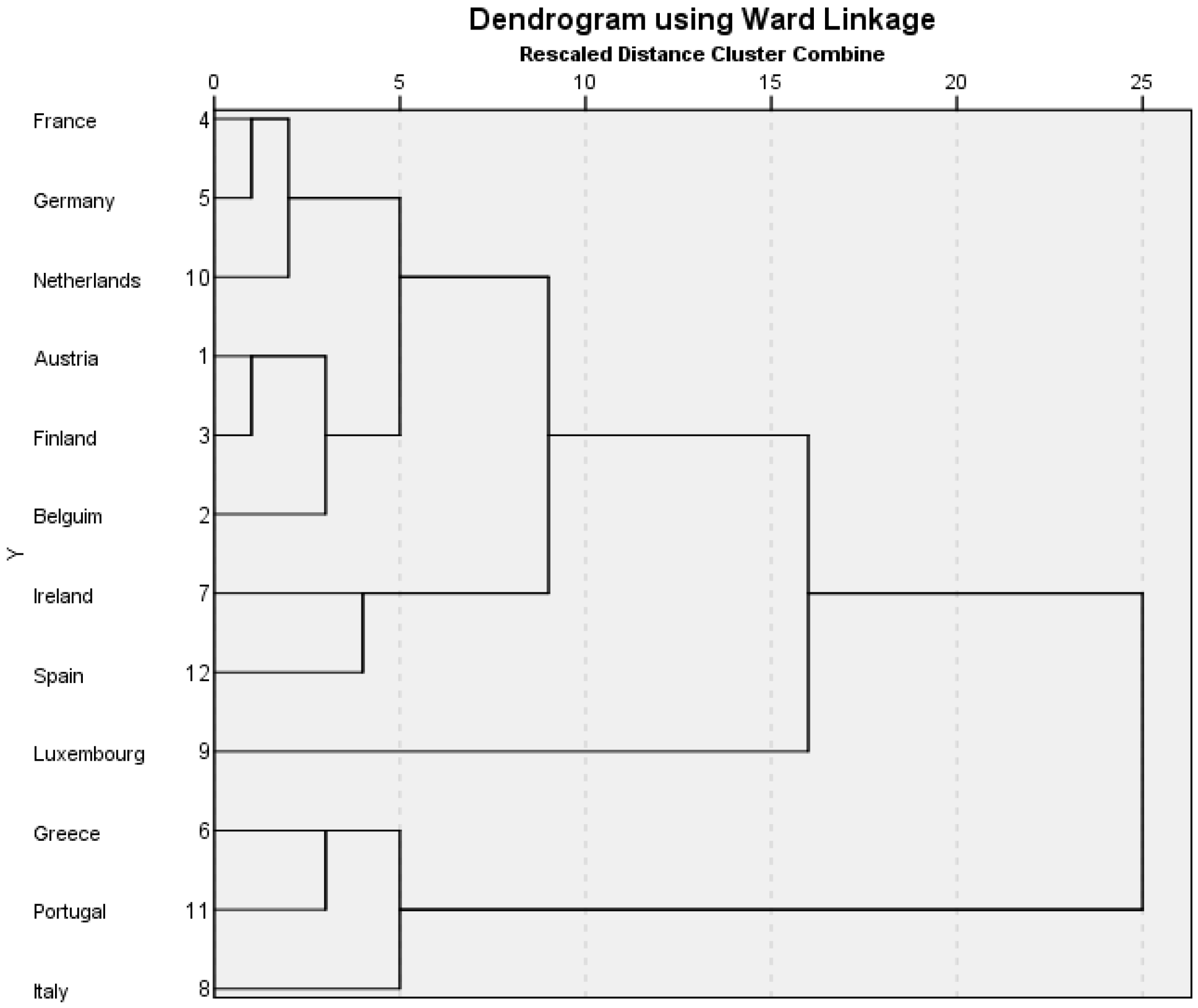
Figure 1 shows the results of the cluster analysis for the first time period, 2002, using the twelve countries who were members of the euro at this point. The cluster analysis groups the cases from the left of the dendrogram, according to the basis of their mathematical similarity. If two small groupings are fairly similar, the hierarchical analysis links them together at the next step (this is point 5 on the rescaled distance measure on the horizontal axis). Three main clusters are formed at point 5 on the axis. The first comprises France, Germany, the Netherlands, Austria, Belgium and Finland. The second consists of Ireland and Spain. They share some proximity to the first cluster. The third cluster is Greece, Portugal and Italy. Luxembourg is an outlier.

Table 1. Bivariate relationships with clusters, 2002, ranked by top four Eta Squared effect scores.

	Mean	Median	Standard Deviation	Eta Ƞ2 ANOVA
State Control of Regulation
Cluster 1	2.37	2.30	0.24	Ƞ2 0.83 ANOVA F = 19.76 p = 0.001
Cluster 2	2.49	2.49	0.07
Cluster 3	3.46	3.42	0.33
Total	2.69	2.49	0.55
Consumer Confidence
Cluster 1	−10.42	−9.85	11.65	Ƞ2 0.72 ANOVA F = 10.25 p = 0.01
Cluster 2	−5.65	−5.65	19.59
Cluster 3	−44.73	−44.00	3.56
Total	−18.91	−19.50	19.68
Labour Productivity per hour worked
Cluster 1	127.33	129.75	14.26	Ƞ2 0.62 ANOVA F = 6.64 p = 0.02
Cluster 2	110.45	110.45	11.95
Cluster 3	83.47	79.80	24.11
Total	112.30	113.40	24.86
HICP
Cluster 1	2.07	1.80	0.93	Ƞ2 0.57 ANOVA F = 5.41 p = 0.03
Cluster 2	4.15	4.15	0.78
Cluster 3	3.40	3.70	0.70
Total	2.81	2.60	1.17

explores the variable influences on the cluster formation.

Four variables were found to have a strong influence on the definition of the clusters (Table 1). These are: state control of regulation, labour productivity per hour worked, consumer confidence and HICP.

Table 1 shows that the Northern cluster (cluster 1) has a lower average score for state control of regulation (2.37). The pairing of Spain and Ireland (2.49) are also slightly below the sample mean (2.69). The notable difference is with the third cluster of Greece, Portugal and Italy (3.46). Likewise cluster 3 has a much lower consumer confidence score (−44.73) than the other clusters (sample average −18.91). The Northern cluster 1 is also differentiated from other countries by its high labour productivity rate (127.33) compared to the sample average of 112.30.

Spain and Ireland (cluster 2) have the highest consumer confidence score (−5.65) compared to a sample average of −18.91. HICP inflation is highest in cluster 2 (4.15%), compared to the average of the other countries (2.81%). The Northern European cluster has the lowest HICP of the three clusters (2.07%). Summary definitions of the 2002 clusters are described in

Table 2. Qualitative summary definition of 2002 clusters.

Cluster 1 High productivity, low inflation, low regulation, average confidence

Austria, Belgium, France, Germany, Netherlands, Finland

Cluster 2 Average productivity, high inflation, average regulation, high confidence

Ireland, Spain

Cluster 3 Low productivity, average inflation, high regulation, low confidence

Greece, Portugal, Italy

below.

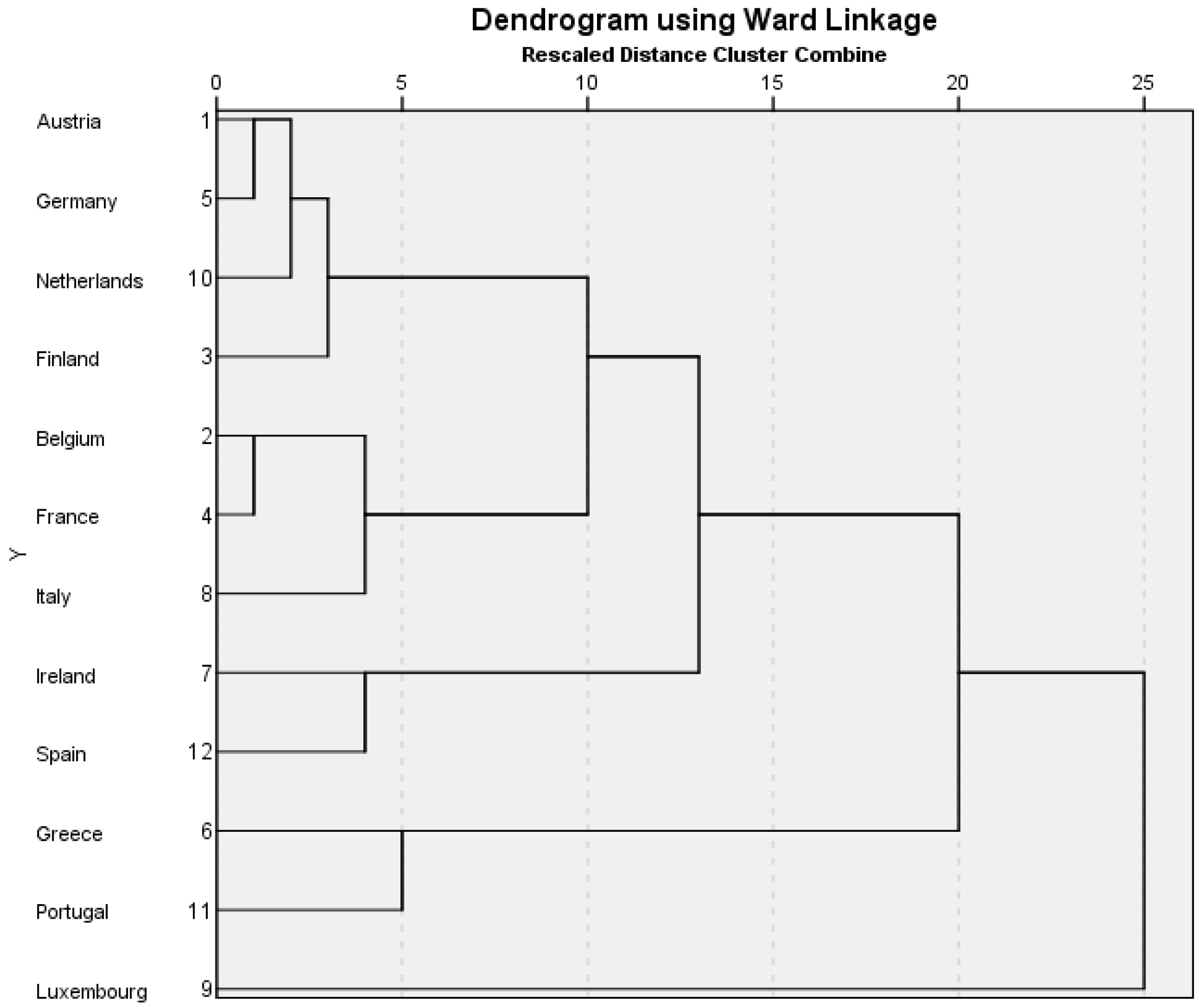
In the 2006 (Figure 2) cluster model there are three predominant clusters and Luxembourg remains an outlier. The first cluster is comprised of Austria, Germany, the Netherlands, Finland, Belgium, France and Italy. The second is the pairing of Ireland and Spain. The third is the pairing of Greece and Portugal.

In 2006 (Figure 2) there appears to be more relative convergence when compared to 2002 (Figure 1). Italy is linked to cluster 1, the Northern cluster, and this cluster has some limited proximity to Spain and Ireland (cluster 2, Figure 2).

The four variables that make the most contribution to defining the 2006 clusters (

Table 3. Bivariate relationships with clusters, 2006, ranked by top four Eta Squared effect scores.

	Mean	Median	Standard Deviation	Eta Ƞ2 ANOVA
Total investment all sectors, percentage of GDP invested
Cluster 1	21.82	22.35	1.05	Ƞ2 0.95 ANOVA F = 71.66 p = 0.001
Cluster 2	31.02	31.02	0.04
Cluster 3	23.09	23.09	0.84
Total	23.73	22.50	3.74
HICP
Cluster 1	1.84	1.80	0.33	Ƞ2 0.79 ANOVA F = 15.43 p = 0.001
Cluster 2	3.15	3.15	0.64
Cluster 3	3.15	3.15	0.21
Total	2.32	2.20	0.74
Labour productivity per hour worked
Cluster 1	122.26	127.40	14.11	Ƞ2 = 0.74 ANOVA F = 11.21 p = 0.001
Cluster 2	111.40	111.40	12.59
Cluster 3	70.80	70.80	10.75
Total	110.93	114.10	23.64
Export to Import ratio
Cluster 1	1.06	1.10	0.07	Ƞ2 = 0.66 ANOVA F = 7.73 p = 0.01
Cluster 2	0.97	0.97	0.23
Cluster 3	0.72	0.72	0.08
Total	0.99	1.05	0.16

) are: total investment, HICP, labour productivity and export to import ratio. Labour productivity and HICP are the remaining strong variable influences from the 2002 model.

For total investment as a percentage of GDP, Greece and Portugal (23.09%) are close to Northern Europe with Italy, in cluster 1 (21.82%). Spain and Ireland are higher at (31.02%). But for HICP inflation scores, Spain and Ireland are similar to Greece and Portugal (3.15%). Northern Europe with Italy enjoys low inflation (1.84%). Northern Europe with Italy have the highest average productivity score (122.26), also close to Spain and Ireland (111.40), but higher than Greece and Portugal (70.80). This cluster pattern is repeated with the export to import ratio averages, where Northern Europe with Italy scores 1.06, close in proximity to Spain and Ireland (0.97), and Greece and Portugal have a lower average of 0.72. Summary definitions of the 2006 clusters are described in

Table 4. Qualitative summary definition of 2006 clusters.

Cluster 1 Average investment, low HICP, high productivity and exporting.

Austria, Germany, Netherlands, Finland, Belgium, France, Italy

Cluster 2 High investment, high HICP, average productivity, trade balance

Spain, Ireland

Cluster 3 Average investment, high HICP, low productivity, importing

Greece, Portugal

Outlier

Luxembourg

.

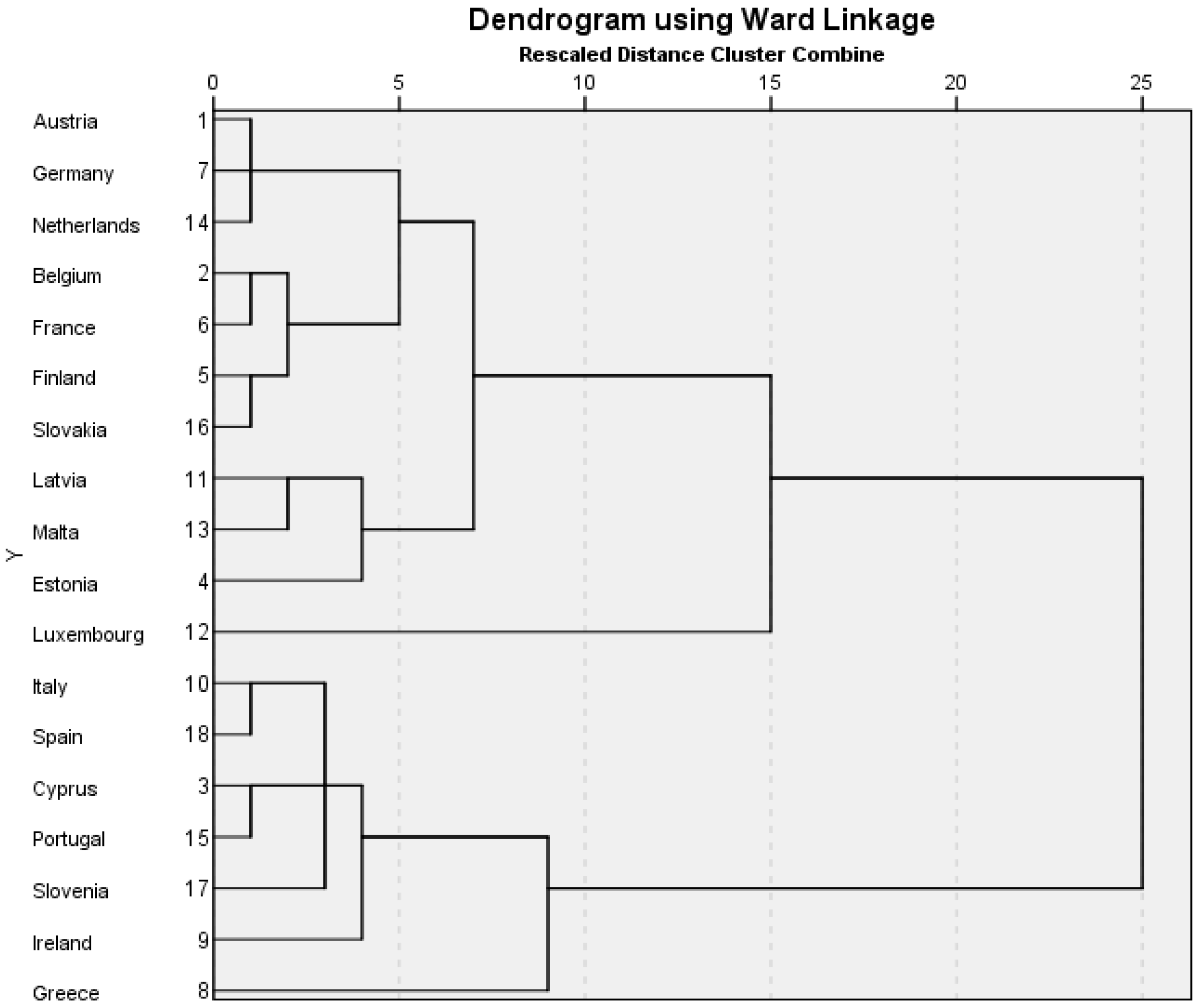
The 2013 model includes the countries that had joined the euro by that year. There are two outliers that are not sufficiently similar to any of the groupings and these are Luxembourg and Greece. The model shows cluster 1 as retaining the core countries of Austria, Germany, the Netherlands, Belgium, France and Finland. They are joined by a new member, Slovakia. The second cluster is comprised of three new, small economies: Latvia, Malta and Estonia. The third cluster includes Italy, Spain, Portugal and Ireland. They are joined by the new euro members of Slovenia and Cyprus.

Table 5. Bivariate relationships with clusters, 2013, ranked by top four Eta Squared effect scores.

	Mean	Median	Standard Deviation	Eta Ƞ2 ANOVA
Long Term Interest Rates
Cluster 1	2.17	2.02	0.52	Ƞ2 = 0.77 F = 22.33 p = 0.001
Cluster 2	3.68	3.36	0.57
Cluster 3	5.21	5.18	1.13
Total	3.59	3.35	1.60
GDP annual percentage change
Cluster 1	−0.03	0.20	0.79	Ƞ2 = 0.69 F = 14.68 p = 0.001
Cluster 2	3.07	2.90	0.96
Cluster 3	−1.88	−1.30	1.80
Total	−0.14	−0.05	2.17
Labour productivity per hour worked
Cluster 1	116.31	126.40	20.01	Ƞ2 = 0.64 F = 11.71 p = 0.001
Cluster 2	39.43	56.90	34.22
Cluster 3	94.43	93.90	20.73
Total	93.69	103.60	35.88
Government Gross Debt
Cluster 1	76.26	74.50	17.10	Ƞ2 = 0.64 F = 10.22 p = 0.002
Cluster 2	40.37	38.10	31.56
Cluster 3	110.43	117.70	23.61
Total	82.34	76.45	103.60

shows the main variable influences on the cluster formations. The only variable to remain influential on both the 2006 and 2013 models is labour productivity per hour worked. Cluster 1 has above average labour productivity (116.31), cluster 2 (39.43) is substantially below the euro sample average (93.99) and cluster 3 has average productivity (94.43). Cluster 1 has below average long term interest rates (2.17), cluster 2 (3.68) has very close to average for the euro group (3.59) and cluster 3 has higher long term interest rates (5.21). Cluster 1 has close to average GDP annual percentage change (−0.03%), while cluster 2 has above average (3.07%) and cluster 3 is below average (−1.88%). Finally, gross government debt as a percentage of GDP is close to the euro average (82.34%) in cluster 1 (76.26%), below average (40.37%) in cluster 2 and above average (110.43%) in cluster 3. A summary statement of the difference between clusters is shown in

Table 6. Qualitative summary definition of 2013 clusters.

Cluster 1 Low interest rates, average GDP growth, high labour productivity, average government gross debt.

Austria, Germany, Netherlands, Belgium, France, Finland, Slovakia

Cluster 2 Average interest rates, high GDP growth, low labour productivity, low gross government

Latvia, Malta, Estonia

Cluster 3 High interest rates, low GDP growth, average labour productivity, high gross government debt

Italy, Spain, Cyprus, Portugal, Slovenia, Ireland

Outliers

Luxembourg, Greece

.

Table 7. Truth Table: Clusters for 2013: Detailed analysis of sub clusters. v1: LabourProductivity; v2: GDP2013; v3: GovCA2013; v4: GrossGovDebt2013; v5: CustomerConfidence2013; v6: LTIR2013; O: Cluster2013; id: Country.

v1	v2	v3	v4	v5	v6	Cluster	id
1	1	1	0	1	0	0	Luxembourg
1	1	1	0	1	0	1	Austria
1	1	1	1	1	0	1	Germany
1	0	1	0	0	0	1	Netherlands
1	1	1	1	1	0	1	Belgium
1	1	0	1	0	0	1	France
1	0	1	0	1	0	1	Finland
0	1	1	0	1	0	1	Slovakia
0	1	1	0	0	0	2	Latvia
0	1	1	0	1	0	2	Malta
0	1	1	0	1	1	2	Estonia
0	0	0	1	0	1	3	Italy
1	0	0	1	0	1	3	Spain
0	0	0	1	0	1	3	Cyprus
0	0	0	1	0	1	3	Portugal
1	0	0	1	1	1	3	Ireland
0	0	0	0	0	1	3	Slovenia
0	0	0	1	0	1	0	Greece

demonstrates a full QCA for the 2013 model using all six variables that recorded a bivariate Eta squared score of above 0.5 in their relationship with cluster membership. The ‘crisp set’ QCA truth table (Rihoux and De Meur, 2009 [29]) divides each explanatory variable into a binary grouping where the median value is the point of division. This analysis illustrates the complexity within the broad cluster groups, especially within clusters 1 and 3.

In Figure 3, cluster 1 can be divided into the component parts of Austria, Germany and the Netherlands, in contrast with Belgium, France, Finland and Slovakia. All these countries share low long term interest rates and all of them apart from Slovakia share high labour productivity (Table 7).

Table 7 demonstrates that for cluster 2 in Figure 3, Latvia, Malta and Estonia share a similar profile of threshold scores including above median scores for their government current accounts.

Cluster 3 in Figure 3 shows the pairings of Italy and Spain, and Cyprus and Portugal. Slovenia and Ireland are singletons within this cluster structure. In Table 7, there are strong similarities across the whole cluster 3 structure for threshold scores. The only differentiation between Italy and Spain is Spain being above threshold for labour productivity while Italy is below. Cyprus and Portugal share identical threshold scores. In Figure 3, Ireland appears as an outlier in cluster 3 when compared to the other members. It has the same above threshold score (Table 7) as Spain for labour productivity, but is the only country in cluster 3 to have an above threshold score for consumer confidence. Slovenia is distinct from the rest of cluster 3 (Table 7) due to having a below threshold score for gross government debt as a percentage of GDP. This is a quality it shares with other new Eastern European member countries (Latvia and Estonia) but whom are not in cluster 3.

The advantage of the QCA truth table is that it allows the researcher to have a qualitative overview of the separate variable impact on each country simultaneously rather than depending on the cluster average scores. While the truth table in Table 7 provides the opportunity to examine the detail of variable effects on cluster memberships, it does not give an account of the scale effect of any one variable. Table 7 does not take into account extreme scores. What the binary classification in Table 7 does not show is the scale differentials used in the full cluster analysis (Figure 3). It does not show that Greece will be differentiated as an outlier by its extreme scores on the full distribution of variable scores. The QCA truth table (Table 7) does not take account of extreme scores.

4. Discussion

This research shows some important movement in the relationships between the original euro member countries across the three time periods studied, 2002, 2006 and 2013. Labour productivity per hour worked remained an important variable that influenced country differences at each of the time points studied, but the multi variate approach used also illustrates the complexity of defining country similarities and differences. Austria, Germany, the Netherlands, Belgium, France and Finland remain at the core of the eurozone through the decade, sharing a number of similarities as their economies evolve. They experience low HICP in 2002 and 2006. In 2013, after the financial crisis, they share similar low long term interest rates.

The path travelled by Spain and Ireland on the periphery of the core Northern group is notable. At the launch of the single currency in 2002, Spain and Ireland are closer to the Northern core, suggesting the idea that they might converge towards it, but by 2006 they remain in the same economic location on the cluster proximity modelling with a little more relative distance on the dendrogram (Figure 2) between them and cluster 1. The 2006 model demonstrates that the new single currency allowed Spain and Italy to achieve significant and above average increases in the percentage of GDP. The variable explanation for their inability to become more similar to the Northern core cluster is a lack of progress with reducing HICP and improving productivity. Italy does move into the core cluster 1 in 2006. It has made some progress controlling HICP, but its cluster membership is temporary and does not continue in 2013, due to insufficient change in other variable scores shared by cluster 1. The temporary joining of Italy with cluster 1 in 2006 is evidence of pre-crisis similarity.

The ability of the new Eastern European states, Slovakia, Latvia and Estonia to demonstrate evidence of some similarity with cluster 1 in 2013 (Figure 3, Table 6 and Table 7) is interesting given the context of their joining at the beginning of the financial crisis. Empirical research has demonstrated that the integration of Eastern European credit markets for businesses and households into Western Europe has increased in the last decade. There was greater speed of convergence for higher interest consumer loans rather than loans to non-financial companies and mortgage loan markets (Volda, 2012 [30]). The successful integration of several small countries into the euro is in part due to their specific trade markets and focus, and the context of the geographical area where they are located in the European market place (Grančay, et al., 2015 [31]).

The management of consumer price inflation was the driving policy theme in applied macroeconomics in the lead up to the launch of the single currency and it was, of course, one of the five defining policy criteria for convergence. The HICP variable has a key influence on differentiating cluster definitions in 2002 and 2006, with differences in HICP cluster averages remaining in 2006 (Table 1 and Table 3). The periphery European euro countries in clusters 2 and 3 at this time, outside of the Northern European low inflation core, struggled to meet inflation targets, as shown by their higher than average inflation, but the euro gave them initial opportunities for lower interest rates, cheaper investment and therefore short term growth. Inflation is no longer a major defining feature of macroeconomic difference after the crisis, as shown by the lack of influence of HICP on defining clusters in the 2013 model. Buti and Turrini (2015) [14] at the European Commission and Estrada, et al. (2013) [32] argue that inflation rates did converge over the long term through the preparations for monetary union and into the first decade of the euro. That puts the periodic divergence of HICP in 2006, when inflation was a defining feature of cluster difference, into a longer term perspective (Buti, 2015 [33]).

When focusing on the five key objectives of the Maastricht Treaty, Buti and Turrini (2015) [14] also argue that there was evidence of the convergence of interest rates until the financial crisis of 2008. As the single currency first created lower interest rates, this generated investment opportunity for some of the periphery countries, as shown in the 2006 model (cluster 2: Spain and Ireland, in Figure 2, Table 3 and Table 4). Apparent convergence of nominal interest rates meant that small differences in inflation could make important operational differences in real interest rates. Buti and Turrini (2015) [14] note that this cheaper capital and pre crisis investment did result in growth in the periphery countries of the euro. But the movement of capital to the periphery found a higher inflationary environment there. Competitiveness and productivity did not improve as much as was necessary and bubbles emerged in the property sector in Spain and Ireland (Lynn, 2011 [34]). In the 2006 model (Table 3), countries in cluster 1 were exporting while those in clusters 2 and 3 were importing.

Much of post crisis European economic policy has been defined by keeping those on the periphery of the eurozone, both in geography and performance, within the currency membership. The crises in Greece, Portugal and Cyprus are in part illustrated by the difference in their economic profiles to other clusters in 2013 (Table 7).

The post crisis shift, demonstrated in the 2013 cluster model, evidenced in both market and government performance data, shows historical differences. Some of the newly joined smaller members have achieved integration through their geographical proximity to the Northern European market place and influence (Grančay, et al., 2015 [31]). Buti and Turrini (2015) [14], argue that the post crisis challenges of managing divergence were exacerbated by the lack of structural economic convergence in the preceding years, illustrated by the export to import ratio differences that are a defining feature of clusters in the 2006 model. Balance of trade was not a convergence criterion in the Maastricht Treaty.

Following the IMF and ECB interventions during the financial crisis, the 2013 model in the cluster research shows the divergence of national long term interest rates (Table 5) and their considerable impact on economic divergence. In the 2013 model, long term interest rate differences are a defining feature of cluster difference and this was not the case in the 2002 and 2006 models. This divergence is at a time of ultra-low interest rates at the European Central Bank and there is a mismatch between low central bank rates and variable national rates. The latter is important evidence of divergence post the crisis. Similarly, the divergence of government gross debt as a percentage of GDP in the 2013 model further illustrates the post crisis gulf between aspects of euro country economies. This variable did not discriminate cluster differences in 2002 and 2006.

Overall, the integration of trade and business economic data in cluster modelling, with the more traditional measures of macroeconomic performance, gives credence to the importance of understanding the experience of the business community and consumers alongside government economic policy objectives. It also illustrates the complexity that convergence may occur in some variables and not others, and that these patterns change and evolve over time. The crisis has changed the variables that define divergence and stand in the way of convergence.

There are some important differences in the application of cluster analysis to understand convergence used in this paper when compared to the recent and innovative approach of Irac and Lopez (2015) [10]. Firstly, the choice of multiple variables was different. This paper used a general macroeconomic approach, starting with the Maastricht criteria and then adding eight additional and well established international macroeconomic indicators. Irac and Lopez focused on structural convergence factors with a more comprehensive coverage of regulation, quality of institutions, knowledge and labour mobility. While the macroeconomic indicators used in this paper include some aspects of these, there was not a deliberate plan to replicate their study, but rather the preference was to understand broad macroeconomic changes.

Secondly, Irac and Lopez attempted an innovative technical measurement of ‘within’ and ‘between’ cluster convergence. The method in this paper did not attempt to replicate such a measurement, but preferred to take a qualitative view of the evolution of cluster memberships over the three time periods of 2002, 2006 and 2013. In terms of methodology, this is close to the ideas of ‘configurative complexity’ as discussed by Rihoux and Ragin (2009) [23]. In other words, the observation of complex patterns is argued to be as much about qualitative judgements as quantitative analysis. Reflections on complex data are still used to make such qualititive judgements.

Thirdly, Irac and Lopez focus exclusively on the first 12 countries to join the euro and neglect the later editions and their effect on the dynamic interaction between countries by 2013. This research includes consideration of the real impact of the new euro members.

Fourthly, there is the issue of Irac and Lopez’s findings. Given the differences in methods outlined, the broad similarity of the findings are important. The analysis in this paper confirms the important overall differences of the Southern European euro member countries from those in the north. While Irac and Lopez provide more detailed analysis of what is effecting the structural convergence issues within those two clusters, the analysis in this research—by applying a logical assumption that clusters are always shifting and changing over time—has highlighted important details about the periphery of cluster memberships, especially with regard to the trajectories of countries like Italy, Spain and Ireland.

5. Conclusions

The research in this paper illustrates that there are important differences in the detail of how Southern European countries have evolved inside the euro area. In 2002, at the onset of the currency, Spain is noticeably different given its higher labour productivity and consumer confidence and lower score for state regulation. The most similar country to Spain at that moment in time was Ireland, rather than any of its southern neighbours. Only one variable had a major influence on differentiating euro cluster memberships through all three time periods, 2002, 2006 and 2013. This was labour productivity per hour worked. When some of the Southern European countries have got closer in overall similarity to their Northern partners, improvements in labour productivity are a consideration. In 2006, Spain remained similar to Ireland. Italy had less similarity with Greece and Portugal in 2006 than in 2002, but this is primarily because of its lower inflation.

In 2013, after the financial crisis, Italy and Spain are more similar, while Greece becomes an outlier because of the extent of its differences. After the crisis, Southern European countries share above euro average long term interest rates. Apart from Slovenia, they also share above average gross government debt. For Greece these variable measures are also above average, but the degree of difference on the scale measurements is even further away from the euro average. So while the Southern European countries can be observed to have similar overall economic problems, the scale of these challenges is different. This observation about the degree of difference in Southern European countries also illustrates an important point about the method of using cluster analysis with other patterning methods like QCA. Cluster analysis takes good overall account of issues of scale and the individual country variable scores, while QCA uses simple thresholds to produce aggregate ‘qualitative’ patterns. This illustrates the value of combining cluster analysis with other methods in order to get more fine grained understanding of the differences between countries. While cluster analysis takes good account of the scale of differences, it does not give the observer much information about the separate variable effects. Combined methods allow both aspects to be considered.

This paper seeks to understand the complexity of the euro area as defined by the interactions of countries with each other, and their changing similarities and differences. It is argued that change in countries can best be understood by examining how their scores on several complementary variables change over time. This overcomes some of the limitations of single dependent variable approaches such as Sigma σ and Beta β convergence models. The implications for the development of convergence theory in Economics and Public Policy is that the application of the concept must give credence to the dynamic evolution of countries in their relationships with each other over time. This requires the use of multivariate and matrix methods that can model changing patterns and configurations of similarity and difference.

The convergence of inflation has been argued to be a major achievement in the euro countries, but the financial crisis has substantially changed the focus of European Economic Policy. Now the driving focus has moved to finding a new structural approach to macroeconomic management that can deliver convergence of growth and its benefits to individual citizens. These major changes in economic policy are important aspects as the single currency moves towards the end of its second decade of existence.

The challenge to find the correct blend of monetary and fiscal interventions to achieve the convergence objectives of the euro area remains (Lein-Rupprecht, et al., 2007 [35]; Dabrowski 2015 [36]; Koske, et al., 2015 [37]). In 2015, the Presidents of the European Commission, the Euro Summit, the Euro group, the European Central Bank and the European Parliament set out an agenda for a further package of policies to deepen convergence of the Economic and Monetary Union (Juncker, 2015 [38]). These measures entail a revised approach to the economic governance coordination, the introduction of national competitiveness boards, an advisory European Fiscal Board, a more unified representation of the euro area in international markets, and the final steps to complete a financial union, notably via a single deposit insurance scheme and a renewed emphasis on building a single market for capital. This policy programme puts the emphasis on ‘sustainable convergence’, with a renewed effort for member states to converge towards best performance and practices in Europe in terms of economic structures, in the first stage, and, in a second stage, formalising a set of commonly agreed legal standards. There are still important details to be formulated about how this policy will be implemented. Rockoff’s (2000) [3] review of the economic history of the establishment of the dollar in the United States concluded that it was vital to set up strong and interventing institutions that could make inter-regional transfers and be a lender of last resort which was sensitive to regional differences. It took the US dollar 150 years to become an OCA, so European institutions will have to provide strong leadership and interventions to quicken the convergence processes. While the first decade of the euro achieved an overall stability in prices, the second decade will most likely be judged by its ability to deliver some convergence and stability in GDP per capita.