Article

Regulating Private Tutoring: Human Capital Formation, Inequality, and Intergenerational Mobility

Graduate School of Economics and Business, Hokkaido University, Kita 9, Nishi 7, Kita-ku, Sapporo 060-0809, Japan
Economies 2026, 14(9), 415; https://doi.org/10.3390/economies14090415 (registering DOI)
Submission received: 6 August 2026 / Revised: 10 September 2026 / Accepted: 14 September 2026 / Published: 17 September 2026
(This article belongs to the Special Issue Development Economics: New Perspectives, Evidence and Challenges)

Abstract

This paper develops a quantitative partial-equilibrium overlapping-generations model to study how private tutoring regulation affects human capital formation, household welfare, educational inequality, and intergenerational mobility. The analysis is motivated by a broader development-economics concern: how unequal access to complementary educational investment interacts with competitive education systems to shape the intergenerational distribution of economic opportunities. The model features heterogeneous households, endogenous ranking-based college admission, and intergenerational human capital transmission. Private tutoring can affect exam performance and productive human capital differently, which allows the analysis to distinguish its competitive and productive roles. Calibrated to Chinese microdata and reduced-form empirical evidence, the model is used as a benchmark quantitative exercise to compare a complete ban, a ban with imperfect enforcement and black-market tutoring, and a welfare-selected tutoring tax that partly finances public education. In the benchmark calibration, a complete ban generates large model-implied welfare and human-capital losses, especially when tutoring contributes to productive skills. Imperfect enforcement preserves part of tutoring activity but can widen group differences in access when informal tutoring costs vary across household types. Among the specific policy experiments considered, the tutoring tax performs better than prohibition-based policies while keeping mean child human capital close to the baseline. This ranking is conditional on the assumed enforcement and public-financing arrangements. The results highlight how education regulation, household heterogeneity, and public-finance design interact in shaping human-capital accumulation and inequality.

1. Introduction

Private supplementary tutoring has become a quantitatively important component of household education investment in both developed and developing economies (Bray, 2006; W. Zhang & Bray, 2020; Hajar & Karakus, 2022). Its rapid expansion has attracted growing policy attention because access to tutoring is strongly associated with household income and parental background, which can reinforce educational inequality (S. Kim & Lee, 2010; Liu & Bray, 2017; Zwier et al., 2020; Matsuoka, 2018). At the same time, tutoring may intensify educational competition and increase pressure on students, raising broader concerns about well-being and resource allocation (Pan et al., 2022; T. Kim et al., 2022; Zheng et al., 2020). Recent studies also show that the COVID-19 period accelerated changes in the organization and delivery of private supplementary tutoring, particularly through the expansion of online provision, while more recent international evidence continues to document substantial variation across countries and education systems in the role and consequences of private tutoring (J. C. Lee et al., 2023; Karakus et al., 2024; Bray, 2024).
A central challenge for policy evaluation is that it remains unclear whether private tutoring primarily builds productive human capital or mainly improves exam performance. While some studies find positive effects on academic outcomes, others show limited or heterogeneous effects once selection and endogeneity are taken into account (Y. Zhang, 2013; Kuan, 2011; Sun et al., 2020). Existing evidence further suggests that tutoring may improve exam performance more than long-run productive human capital. Dang and Rogers (2008) emphasize that even participating households may be uncertain about whether tutoring generates genuine productive gains or mainly improves performance in competitive examinations, although tutoring need not be entirely wasteful. Guo et al. (2020), by contrast, provide more direct evidence that tutoring primarily raises subject-specific and exam-related performance, with much weaker effects on broader cognitive ability. This distinction is crucial because the desirability of regulation depends on whether tutoring mainly builds productive skills or mainly strengthens relative position.
This issue is especially important in high-stakes, ranking-based admission systems. In such settings, educational success depends not only on absolute achievement but also on relative performance in competition for limited slots in higher-quality schools and universities. A growing literature shows that tutoring is closely tied to selective educational transitions and ranking-based allocation (Guill & Lintorf, 2019; Zwier et al., 2020; Stevenson & Baker, 1992; Buchmann et al., 2010). This structure gives households incentives to invest in tutoring even when its contribution to long-run productivity is uncertain, and can turn educational investment into a form of positional competition (Ramey & Ramey, 2010).
The broader economics literature has studied closely related mechanisms through models of parental investment and intergenerational human-capital accumulation. Quantitative work in this tradition emphasizes that household resources, parental characteristics, and education policies jointly shape investments in children and thereby affect human-capital formation, inequality, and the persistence of economic status across generations. Abbott et al. (2019), for example, analyze education policy and intergenerational transfers in a life-cycle framework in which parental characteristics and household resources influence children’s skill formation and educational choices. S. Y. Lee and Seshadri (2019) emphasize the role of childhood human-capital investment in generating intergenerational persistence, while Caucutt and Lochner (2020) show how family resources, borrowing constraints, and the timing of parental investment affect children’s human-capital accumulation and mobility. More broadly, Abdulla (2023) highlights the importance of human-capital differences for persistent differences in economic outcomes. Abbott (2022) further emphasizes the role of household heterogeneity in shaping educational investment and long-run outcomes. Together, these studies provide a broader human-capital foundation for understanding how differences in household educational investment can translate into persistent inequality across generations. The present paper builds on these insights but focuses on private tutoring as a distinct form of household education investment and on the additional strategic incentives that arise when scarce educational opportunities are allocated according to relative exam performance.
Recent work has begun to incorporate educational competition into quantitative frameworks. S. Kim et al. (2024) study the role of educational competition in a model of endogenous fertility, where parents care about their children’s outcomes relative to those of other children and competition operates through a status externality in parental preferences. Gu and Zhang (2024) analyze parental investment competition for college admissions in a quantitative model where investment affects both labor productivity and admission outcomes through an empirically estimated admission mapping, and where pre-college human capital may only partially translate into productive adult human capital.
Motivated by these contributions, this paper develops a quantitative framework that endogenizes ranking-based admission competition within a model of household education investment. We build a partial-equilibrium overlapping-generations economy with heterogeneous households in which parents allocate resources across consumption, savings, and private tutoring for their children. Compared with S. Kim et al. (2024), where competition enters parental preferences directly through concern for children’s relative outcomes, parents in our model care about their children’s expected future consumption, and private tutoring matters because it changes admission prospects through an explicitly ranking-based allocation mechanism. Children’s outcomes depend on both public schooling and private tutoring. The central question is how regulation performs when tutoring is partly productive but also improves relative position in a competitive admission system.
The paper makes three related contributions. First, it introduces an endogenous ranking-based admission mechanism that links household tutoring decisions to the economy-wide distribution of exam performance. Second, it separates the exam-related and skill-related effects of tutoring and shows how the policy trade-off changes with the productive value of tutoring. Third, it studies how imperfect enforcement changes the incidence of a ban when access to informal tutoring differs across parental education types. Together, these mechanisms connect private tutoring regulation to broader questions in development economics concerning human-capital formation, inequality of opportunity, and the intergenerational transmission of economic advantage.
We compare three policy regimes: a complete ban on private tutoring, a ban with imperfect enforcement and black-market tutoring, and a tutoring tax whose revenue partly replaces the common contribution used to finance public education. In the benchmark calibration, prohibition-based policies generate large model-implied welfare and human-capital losses when tutoring contributes to productive skills. Unequal informal access partly preserves tutoring activity but creates additional differences in participation across household groups. The welfare-selected tutoring tax performs better among the specific policy experiments considered. This comparison is conditional on the model’s enforcement and financing assumptions: the tax is optimized over a grid and assumed to be collected effectively, whereas the prohibition experiments use fixed enforcement structures. China provides the data and institutional motivation for the benchmark calibration, but the policy exercises are not intended as a direct structural evaluation of a particular observed reform. In particular, the tutoring tax is a counterfactual policy instrument rather than a description of current Chinese policy. Although the quantitative magnitudes are specific to the Chinese calibration, the underlying mechanisms are relevant to other education systems in which households can purchase supplementary instruction and access to scarce educational opportunities depends partly on relative academic performance.
The remainder of the paper is organized as follows. Section 2 presents the model. Section 3 describes the calibration strategy. Section 4 reports the main quantitative results and policy comparisons. Section 5 provides three counterfactual experiments. Section 6 discusses the robustness. Section 7 discusses interpretation and limitations. Section 8 concludes.

2. The Model

We develop a partial-equilibrium overlapping-generations (OLG) model to study how policies regulating private tutoring affect household behavior, educational investment, and intergenerational human capital dynamics. The model features a continuum of heterogeneous households, endogenous ranking-based college admission, and policy interventions that change the cost and accessibility of private tutoring.

2.1. Household Problem

In each generation, a parent chooses consumption, savings, and private tutoring expenditure for a child to maximize lifetime utility:
max c , c , s , p c 1 ρ 1 ρ + β c 1 ρ 1 ρ + γ c ˜ 1 ρ 1 ρ s . t . c + s + τ p + c j p t ( p ) = w h p ξ , c = ( 1 + r δ ) s .
Here, c and c denote first- and second-period consumption, s denotes savings, and p denotes private tutoring expenditure for the child. The term c ˜ denotes the child’s expected lifetime-consumption index, obtained from the consumption policy associated with the child’s expected adult human capital. It enters parental utility through altruistic preferences.1 The parameter 1 / ρ is the intertemporal elasticity of substitution, β is the discount factor, and γ captures parental altruism.
Household income is given by w h p ξ , where w is the wage rate, h p is parental human capital, and ξ is a multiplicative residual earnings component not explained by h p .2 The parameter r denotes the interest rate, and δ is the depreciation rate of savings. The term τ p is a common contribution used to finance public education. The function c j p t ( p ) denotes the total cost of private tutoring and may depend on policy and the parent’s previously realized education type j p , as specified below.

2.2. Human Capital Formation

Human capital formation has four components: intergenerational inheritance, pre-college human capital accumulation, college admission, and post-college human capital realization. The child inherits human capital from the parent according to
h i n h = θ h p + ε , ε N ( 0 , σ 2 ) ,
where θ captures intergenerational persistence and σ governs the dispersion of the inheritance shock.
Before college admission, the child accumulates two forms of pre-college human capital. The first is exam-relevant human capital, which determines the child’s position in the admission system:
h e x a m = h i n h + T ( e s , p ) ,
where e s denotes fixed public education expenditure. The second is skill-relevant human capital, which affects long-run productivity:
h p r e = h i n h + T ( e s , ω p ) .
The education production function is
T ( e s , x ) = A λ e s μ + ( 1 λ ) x μ 1 / μ .
Here, A is a scale parameter, λ governs the relative contribution of public education, and μ determines the elasticity of substitution between public education and private tutoring.3 The parameter ω [ 0 , 1 ] measures the extent to which private tutoring contributes to skill-relevant human capital relative to exam performance. A higher ω implies that tutoring is more productive in the long run, while a lower ω implies that tutoring mainly improves exam outcomes.4
College admission depends on the child’s position in the economy-wide distribution of exam-relevant human capital. Let
κ = F ( h e x a m ) [ 0 , 1 ]
denote the child’s percentile rank in this distribution. The ranking is determined endogenously by the equilibrium distribution of exam-relevant human capital across households, and only relative rank matters for admission in the model.
There are three possible education tracks for the child: no college ( j c = 0 ) , non-selective college ( j c = 1 ) , and selective college ( j c = 2 ) . Admission probabilities π j c are given by
π 2 = Λ κ q 2 b , π 1 = Λ κ q 1 b Λ κ q 2 b , π 0 = 1 Λ κ q 1 b ,
where
Λ ( x ) = 1 1 + e x .
Here, q 1 and q 2 are the admission thresholds for non-selective and selective colleges, and b controls the smoothness of the admission function.5
Given these admission probabilities, the child’s expected human capital is
E [ h ] = h p r e 1 + π 1 Δ 1 + π 2 Δ 2 .
Here, Δ j c is the model-implied earnings premium associated with the child’s realized education track j c . After the education track is realized, post-college human capital is given by
h = h p r e ( 1 + Δ j c ) + η j c , j c { 0 , 1 , 2 } ,
where η j c is an idiosyncratic productivity shock. This realized human capital becomes parental human capital in the next generation.

2.3. Policy Environment

We now specify the tutoring cost introduced in the household problem. The total tutoring cost for a parent of type j p is
c j p t ( p ) = ( 1 + p 0 + φ a j p ) p , j p = 0 , 1 , 2 .
The parameter p 0 is a baseline reduced-form cost wedge that captures search, coordination, transportation, and other non-tuition costs of using tutoring. The parameter φ [ 0 , ) represents enforcement intensity: a higher value raises the effective cost of obtaining tutoring under regulation. When φ = 0 , the economy corresponds to the baseline without tutoring regulation, and tutoring is available at cost ( 1 + p 0 ) p . When 0 < φ < , private tutoring is officially restricted but imperfectly enforced, so households can still obtain tutoring at higher and type-dependent costs. As φ , tutoring becomes prohibitively costly and households optimally choose p = 0 , corresponding to a strict ban. The scenario parameters a j p govern type-specific costs of informal access, with
a 0 > a 1 > a 2 .
This ordering assumes that parents with higher previous education have better information or social connections and therefore face lower effective costs under regulation.6
In addition to quantity-based regulation, we consider a price-based policy in which private tutoring is taxed rather than restricted. Under this policy, we set φ = 0 and introduce a proportional tutoring tax rate τ t . The total tutoring cost becomes
c j p t ( p ) = ( 1 + p 0 ) ( 1 + τ t ) p .
For each benchmark environment, τ t is selected from a fixed grid to maximize average model utility. The reported tax is therefore the best-performing tax within the grid, whereas the prohibition experiments use fixed enforcement structures.7
Tutoring tax revenue is used to finance public education, with average revenue given by
g = E τ t ( 1 + p 0 ) p .
Total public education expenditure remains fixed at e s and is jointly financed by the common contribution τ p and tutoring tax revenue:
e s = τ p + g .
The tax therefore operates through two channels. It raises the private cost of tutoring and reduces the common contribution required to finance public education. The resulting welfare effect combines a change in tutoring incentives with a change in the distribution of the financing burden.

2.4. Timing and Equilibrium

The timing within each generation is as follows. A parent enters the period with human capital h p and a previously realized education type j p , and draws the residual earnings component ξ . Given the policy environment, the common public education contribution, and the reference distribution of exam performance, the parent chooses consumption, savings, and tutoring expenditure.
Public education and tutoring then determine the child’s exam-relevant and skill-relevant human capital. The child’s exam-relevant human capital is mapped into a percentile rank using the economy-wide distribution F. This rank determines the probabilities of entering the three education tracks. The child’s education track and productivity shock are then realized, determining adult human capital. The resulting human capital and education type become ( h p , j p ) for the next generation.
Thus, ( h p , j p , ξ ) are household-level states, while ( c , c , s , p ) are household choices. The distribution F is an aggregate equilibrium object. Individual households take it as given when choosing tutoring expenditure, while the distribution generated by all household decisions must be consistent with the distribution used to form percentile ranks. The numerical procedure iterates on this distribution until convergence.

3. Calibration

The calibration proceeds in three steps. First, a set of parameters is fixed externally using normalization, institutional information, and directly observed statistics. Second, another set is disciplined by reduced-form empirical relationships estimated outside the model. Third, the remaining parameters are internally calibrated by matching model-implied moments to their empirical counterparts. Further details are provided in Appendix D.

3.1. Data

The empirical analysis uses microdata from the China Family Panel Studies (CFPS) for the 2010–2022 waves. We construct a unified individual-level dataset by merging adult and child records, linking them to household identifiers through the family relationship files, and adding household economic information from the family economic files. Since variable definitions differ across waves, we make the key variables consistent across waves. All monetary variables are deflated using province-level consumer price index (CPI) data and expressed in real terms with 2010 as the base year. Household-level variables are then adjusted using the OECD-modified equivalence scale and normalized into model units.8

3.2. Descriptive Trends in Private Tutoring

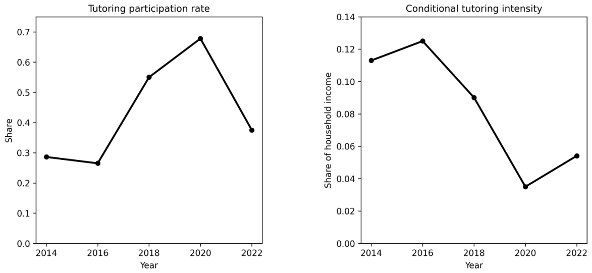
Before turning to the calibration, we document the evolution of private tutoring in the CFPS. Figure 1 reports tutoring participation and conditional tutoring intensity among children aged 12–18 for the harmonized survey waves from 2014 to 2022. Tutoring participation is defined as reporting positive tutoring expenditure or participation in tutoring classes. Conditional tutoring intensity is measured as tutoring expenditure relative to household income among participating households.9
The data reveal a pronounced expansion of private tutoring before 2020. Participation remained at around 27–29% in 2014–2016, but then rose rapidly to 55.0% in 2018 and 67.8% in 2020. By 2022, however, the participation rate had fallen sharply to 37.5%. This reversal coincides with a major change in China’s tutoring-policy environment. The “Double Reduction” policy introduced in 2021 imposed extensive restrictions on subject-based off-campus tutoring, while the COVID-19 period also altered the availability and delivery of supplementary tutoring, particularly through the expansion of online provision (J. C. Lee et al., 2023; Karakus et al., 2024). The 2022 decline should therefore be interpreted as a descriptive pattern that is consistent with these institutional and market disruptions rather than as a causal estimate of either effect.
Conditional tutoring intensity followed a different trajectory. Among participating households, tutoring expenditure accounted for approximately 11–13% of household income in 2014–2016, declining to 9.0% in 2018 and 3.5% in 2020 before increasing modestly to 5.4% in 2022. Taken together, the two panels show that the rapid pre-2020 expansion of tutoring occurred mainly along the extensive margin, while the share of income spent by participating households generally declined. These changes provide empirical context for the model’s emphasis on tutoring participation, expenditure intensity, and policy regulation.

3.3. Externally Fixed and Benchmark Parameters

We first fix a set of parameters using normalization, institutional information, and direct measurement from the data. These parameters are reported in Table 1.
The wage rate w is normalized to one, which defines the unit of measurement in the model. Specifically, all monetary variables are converted into real, equivalized terms and normalized by the weighted median of household wage income in 2010.10 Public education expenditure e s is measured from household-level school education expenditures for households with children in public schools, using the weighted median across household-year observations from the 2016–2022 waves. The net return on savings, r δ , is set to 0.02, consistent with observed real interest rates. Parameters q 1 and q 2 are benchmark admission thresholds for the two college tracks.11 Finally, φ , a 0 , a 1 , and a 2 are benchmark scenario parameters rather than quantities directly estimated from underground tutoring markets. The benchmark enforcement intensity φ represents an intermediate case in which regulation substantially raises the effective cost of tutoring but does not eliminate informal participation. The values of a 0 , a 1 , and a 2 represent a plausible ordering of informal access across parental types. The quantitative importance of both enforcement intensity and unequal access is assessed over wider ranges in Section 5.

3.4. Parameters Disciplined by Reduced-Form Evidence

We next discipline a set of parameters using reduced-form empirical relationships estimated from the data. These relationships provide benchmark mappings rather than structural or causal identification, and the resulting values are treated as fixed inputs in the baseline calibration. Accordingly, these estimates should be interpreted as empirically anchored benchmark parameters rather than precisely identified structural primitives. The robustness exercises therefore examine how the main policy conclusions change when the less precisely disciplined parameters are varied. Table 2 reports their values.
The parameter ω governs the extent to which private tutoring contributes to skill-relevant human capital, as distinct from exam performance. We construct a benchmark value by comparing conditional associations between tutoring expenditure and more exam-oriented outcomes, such as mathematics and language scores, with associations for broader cognitive measures, such as memory and digit span. The former are used as proxies for exam-related performance, while the latter are used as proxies for broader skill formation.12 We then map the relative strength of these associations into ω .
The parameters θ and σ are anchored by the conditional parent–child relationship in completed education and its residual dispersion. These reduced-form moments contain inherited, family, investment, and institutional channels, so they should be interpreted as empirical disciplines on overall intergenerational persistence rather than pure measures of inherited ability. The parameters Δ j c are mapped from conditional earnings differences across education groups, while the dispersion parameters η j c use within-group residual variation. The earnings differences may include selection into education and are therefore interpreted as model-consistent earnings premia rather than causal returns to college.

3.5. Internally Calibrated Parameters

The remaining parameters are jointly calibrated to match a set of moments capturing household behavior, human capital accumulation, and the interaction between educational investment and economic heterogeneity. These moments include tutoring participation, tutoring intensity, average human capital, admission sensitivity, and the income gradient in tutoring participation. Table 3 reports the calibrated values.
Tutoring participation is the share of households that engage in private tutoring. Tutoring intensity is the average share of income spent on tutoring among participating households, excluding extreme values. Admission sensitivity measures the gap in college attendance probabilities between students in the top 20% and bottom 20% of the distribution of standardized exam-related human capital.13 The income gradient in tutoring participation captures how tutoring participation varies across the income distribution. It is constructed by sorting households by income, removing extremes, dividing the remaining sample into five groups, and taking the difference between the average participation rate in the top two groups and that in the bottom two groups. These moments are jointly targeted using a numerical optimization procedure, and the model matches most targeted moments closely.14

3.6. Non-Targeted Moments

We further assess the model using a non-targeted income distribution. Table 4 reports selected quantiles in the data and in the model.
The model reproduces the broad shape of the income distribution reasonably well. This comparison is a limited diagnostic rather than a strong external validation, because the income distribution is closely related to the model’s initial heterogeneity and earnings components. The more policy-relevant fit is therefore assessed mainly through the targeted tutoring, education, and admission moments reported above.

4. Policy Effects

This section compares the quantitative effects of alternative tutoring regulations in the calibrated economy.15 We consider three policy regimes relative to the baseline: a complete ban, a ban with black-market access, and a tutoring tax. The tutoring-tax rate is selected by a grid search over [ 0 , 0.30 ] with increments of 0.01 to maximize average model utility.16 Welfare is reported as a model-implied consumption-equivalent variation (CEV) based on average lifetime utility; Appendix B gives the exact formula. We first examine aggregate effects and then turn to heterogeneity across parental human-capital groups.

4.1. Aggregate Effects of Tutoring Policies

Table 5 reports the aggregate effects of the alternative policy regimes at the calibrated benchmark. A complete ban generates the largest model-implied welfare loss, sharply lowers mean child human capital, and eliminates tutoring activity. The CEV is much larger than the tutoring expenditure share because it reflects the full utility effect of current consumption, savings, and the child’s expected future consumption over the intergenerational transition. Its magnitude should therefore be interpreted as a model-based welfare measure rather than a direct empirical estimate of an observed ban. Although the ban raises the mobility indicator, this mainly reflects compression in the outcome distribution rather than a broad improvement in absolute outcomes. In particular, higher relative mobility need not imply higher welfare for the bottom group.
Allowing a black market partly mitigates these effects. Relative to a complete ban, the ban-with-black-market regime yields a smaller welfare loss and higher child human capital because some households continue to obtain tutoring through informal channels. Its aggregate income Gini is only modestly higher than under the complete ban. The distributional importance of the black market is therefore clearer in the large group differences in tutoring participation reported below than in the aggregate Gini alone.
The welfare-selected tutoring tax performs better than the prohibition-based policies within the experiments considered. It keeps mean child human capital and tutoring activity close to baseline levels. Its welfare effect, however, combines a price channel with a financing channel, because tutoring-tax revenue partly replaces the common household contribution used to finance public education. To separate these channels, we consider a same-rate counterfactual that retains the benchmark tax rate of τ t = 0.06 but does not recycle tax revenue through public-education finance. The tutoring-price wedge is therefore unchanged, while the household contribution remains at its baseline level.
Table 6 shows that removing revenue recycling changes the CEV from 1.292 % to 2.194 % , while tutoring participation remains almost unchanged. The positive welfare effect of the benchmark tax therefore depends primarily on the financing and redistribution channel rather than on the tutoring-price channel alone. Accordingly, the tax result should be interpreted as conditional on the assumed public-finance arrangement.

4.2. Distributional Effects Across Households

Aggregate results do not show how policy effects differ across households. To examine these distributional effects, Table 7 reports outcomes separately for households in the bottom 30%, middle 40%, and top 30% of the parental human capital distribution.
Under a complete ban, model-implied welfare losses are large for all groups and are most severe for the bottom group. At the same time, the bottom group’s mean child human capital and probability of reaching the top 20% rise slightly, while the largest absolute decline in child human capital occurs among the top group. The resulting increase in mobility therefore mainly reflects compression of the outcome distribution rather than a uniform improvement for disadvantaged households. Mobility is a relative-rank measure, whereas CEV also reflects current consumption, savings, and the child’s expected future consumption. A policy can therefore raise measured mobility while lowering lifetime welfare, especially when the compression is generated by larger losses at the top and reduced household resources across the distribution.
Under the ban with black-market access, outcomes diverge sharply across groups. The top group retains high tutoring participation, whereas participation remains extremely limited for the bottom group. Part of this pattern comes from the endogenous resource gradient, and part comes from the imposed ordering of informal-access costs. Imperfect enforcement therefore does more than weaken the ban: under the benchmark access assumption, it creates an additional source of group inequality that favors high-background households. The access-gap experiment below shows how strongly this conclusion depends on that assumption.
The tutoring tax generates a markedly asymmetric welfare pattern: the bottom group experiences a substantial model-implied gain, while the middle and top groups see only small changes relative to the baseline. Child human capital and tutoring outcomes remain close to baseline levels. The bottom group benefits most because households that purchase little tutoring bear little direct tax burden while benefiting from the reduction in the common public-education contribution. As shown in Table 6, this distributional effect is closely tied to the assumed revenue-recycling mechanism.

4.3. Mechanisms: Why Do Policies Differ?

The policy differences in Table 5 and Table 7 arise because private tutoring has both a productive role and a competitive role. Policies that reduce tutoring may therefore lessen positional competition, but they may also reduce productive investment. The three policy regimes differ in how they trade off these two effects.
A complete ban removes the tutoring margin entirely. This compresses differences in educational investment and raises measured mobility, but it also generates large model-implied welfare losses by eliminating both the productive and competitive uses of tutoring. The middle group experiences the smallest welfare loss under the ban. In the calibrated economy, these households face competitive pressure similar to that of the top group, but have substantially fewer resources. The ban therefore removes not only potential returns to tutoring, but also part of the competitive burden they would otherwise bear.
The black-market regime differs from a strict ban because access to tutoring is no longer eliminated uniformly. Instead, it becomes unequally distributed across households. High-background households retain better access to informal tutoring channels, whereas the middle group still has strong incentives to participate but faces substantially higher effective costs. As a result, the middle group experiences the sharpest drop in tutoring and the largest welfare loss. The bottom group is less affected because its baseline tutoring participation is already low.
The tutoring tax works through prices and education finance rather than prohibition. It discourages tutoring at the margin while preserving market access, and its revenue reduces the common contribution required to finance public education. Because low-background households purchase relatively little tutoring, this financing mechanism benefits them disproportionately. The decomposition in Table 6 confirms that the benchmark welfare advantage of the tax is conditional on this revenue-recycling arrangement.

5. Counterfactual Experiments

This section presents three counterfactual experiments. We examine how the results change when varying (i) the productivity of private tutoring in skill formation, (ii) the level of public education spending, and (iii) the degree of imperfect enforcement in the presence of a black market.

5.1. The Role of Tutoring Efficiency

Table 8 reports outcomes under different values of ω , which governs the contribution of private tutoring to skill formation relative to exam performance. Since this parameter is difficult to measure directly, the counterfactual exercise assesses how policy performance depends on the productive value of tutoring.17
When ω = 0 , tutoring is purely positional. In this case, policies that reduce tutoring mainly curb wasteful competition, so welfare losses become much smaller than in the calibrated case and even turn into gains for the middle group. Mean child human capital also rises slightly, because resources are no longer diverted to non-productive tutoring.
When ω = 1 , tutoring is fully productive. Restricting tutoring then becomes increasingly costly in the model: the tutoring tax is no longer binding and coincides with the baseline, while banning tutoring generates large welfare losses and substantial declines in human capital across all groups. A higher ω also lowers mobility, because higher-income households can convert tutoring more directly into their children’s future productivity.
These results show that the model-based evaluation of tutoring policies depends critically on whether tutoring mainly affects relative rank or productive human capital. Given the limited empirical discipline on ω , the pattern across the full range is more informative than the benchmark point estimate alone.

5.2. Public Education and Policy Interaction

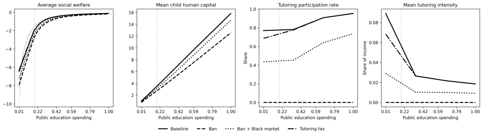
Figure 2 shows how outcomes vary with public education spending e s under different policy regimes.18 Higher public education spending crowds out private tutoring mainly along the intensive margin rather than the extensive margin. As e s increases, mean tutoring intensity declines sharply across policies, while participation often rises. This indicates that stronger public education reduces households’ reliance on intensive tutoring expenditure without necessarily pushing them out of the tutoring market.19

5.3. Black Market Access and Imperfect Enforcement

We next examine how the performance of prohibition depends on imperfect enforcement in the presence of a black market. We consider two parameters: the enforcement intensity φ , which affects the overall cost of tutoring under regulation, and the access gap parameter a g a p , which governs inequality in access to informal tutoring across household types. The benchmark black-market experiment uses φ = 3.5 , while the exercise below varies enforcement intensity over a wider range.20
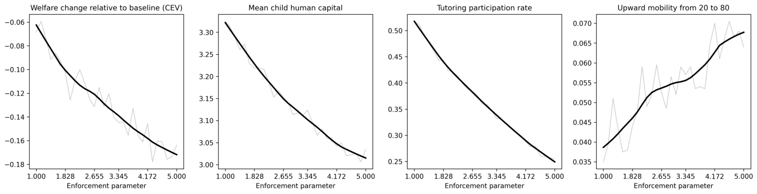
Figure 3 shows that stronger enforcement sharply reduces tutoring participation, lowers human capital and welfare, and raises mobility. Stronger enforcement therefore makes the economy look increasingly like a complete ban, compressing differences in educational investment at the cost of lower efficiency.
Table 9 focuses on the distributional consequences of black-market access. Increasing a g a p raises tutoring participation and improves model-implied aggregate welfare and human capital, because more tutoring activity is preserved for types with lower informal-access costs. However, the distributional effects are not uniform across the range of access inequality. In particular, when the access gap rises beyond the calibrated structure, the improvement in aggregate welfare is driven by gains among the middle and top groups, while the bottom group becomes worse off. The group-specific CEV results therefore show that higher aggregate welfare need not imply welfare gains for all household groups.21

6. Robustness

This section examines the robustness of the results to alternative parameter values. We focus on six key parameters of the model: the efficiency of private tutoring ω , the intergenerational persistence and dispersion parameters θ and σ , the admission thresholds q 1 and q 2 , and the admission smoothness parameter b.

6.1. Tutoring Efficiency

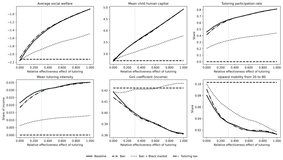
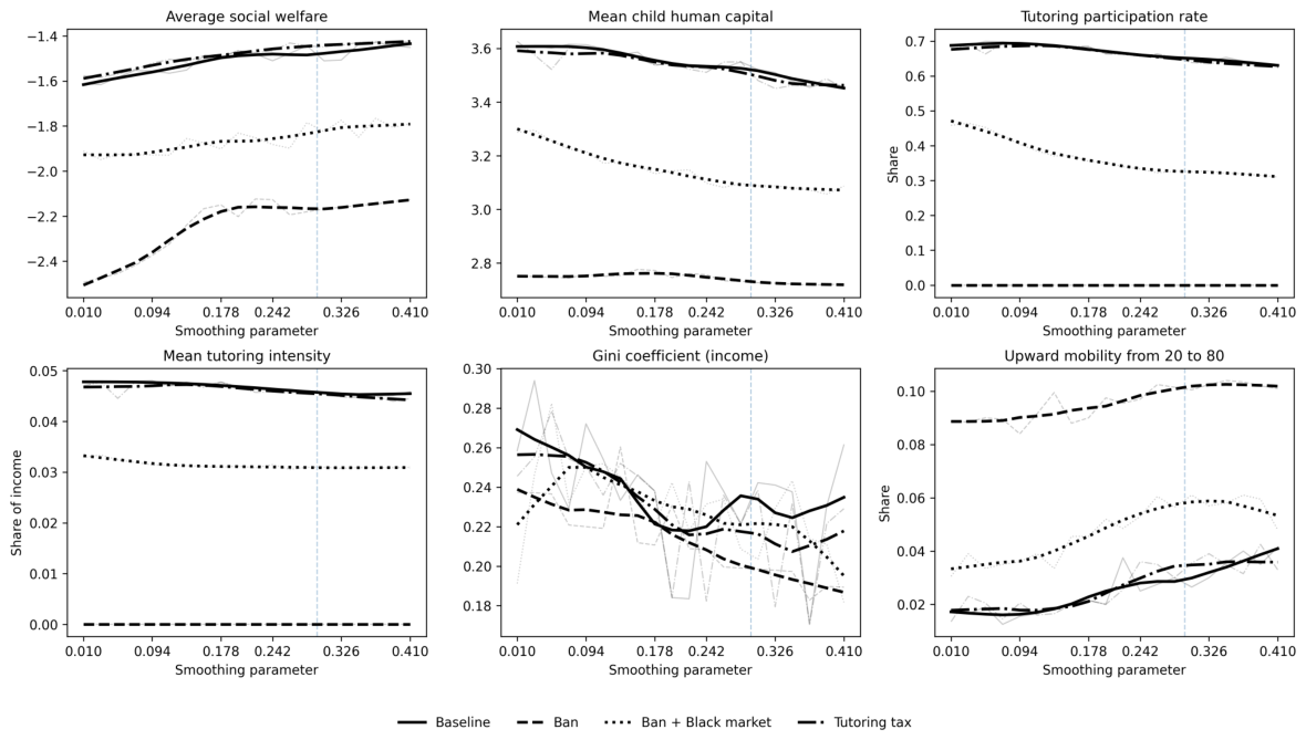
Figure 4 reports results for different values of ω , holding all other parameters fixed. Policies that restrict tutoring generally improve measured mobility but reduce human capital as ω rises, whereas policies that preserve tutoring access generate higher human capital at the cost of lower mobility. The welfare effects change substantially across the range, especially for prohibition. The calibrated value lies in a region where local changes are gradual, but the wider exercise confirms that ω is a central policy parameter rather than a secondary robustness input.

6.2. Intergenerational Transmission

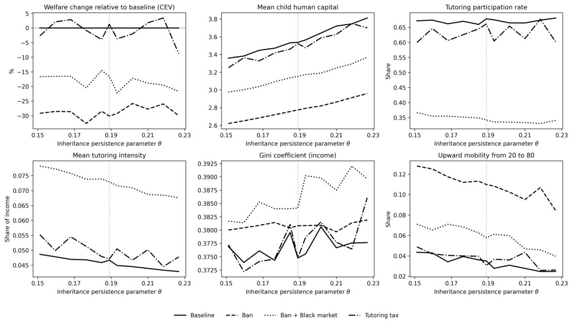
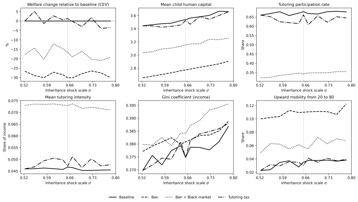
We examine the sensitivity of the results to the intergenerational persistence parameter θ and the dispersion parameter σ . Each parameter is varied separately by approximately ± 20 % around its calibrated value, while all other parameters are held fixed. Figure 5 and Figure 6 show that the main qualitative effects of the prohibition policies remain broadly stable across alternative values of θ and σ . The complete ban continues to generate substantial welfare and human-capital losses, while black-market access mitigates part of these losses. The welfare effect of the tutoring tax is more sensitive to the calibration of intergenerational transmission, especially with respect to σ .

6.3. Admission Thresholds

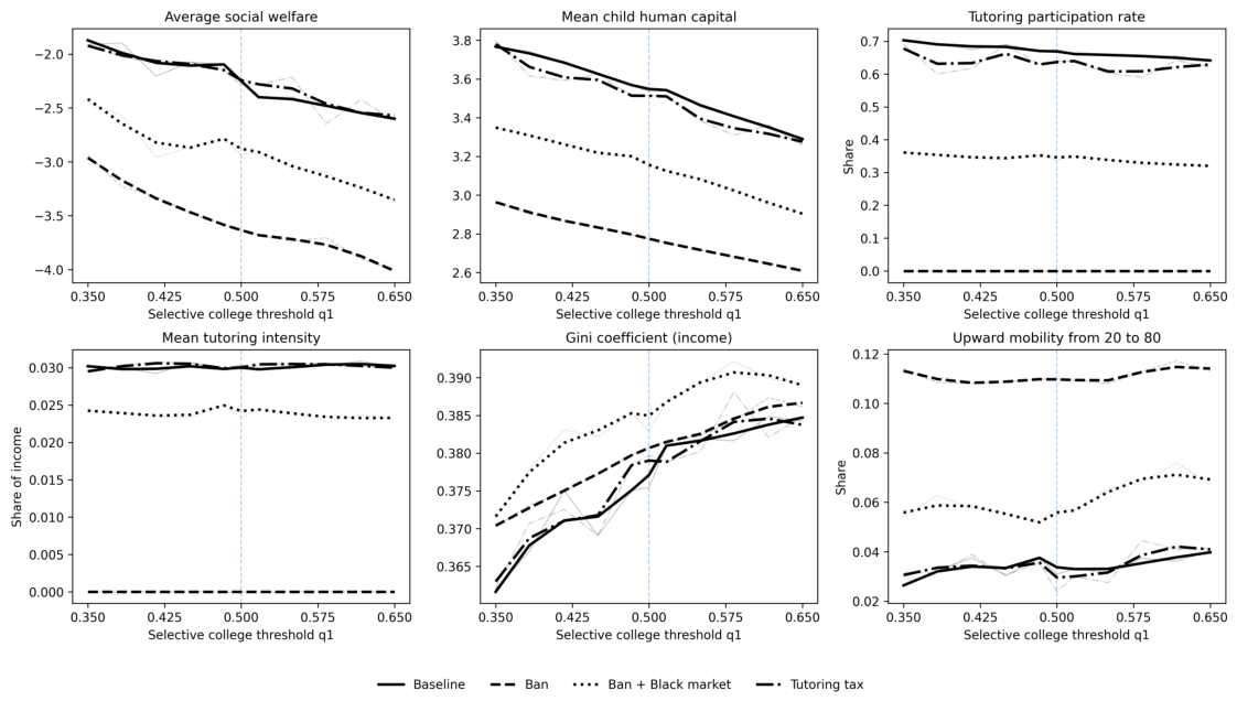
Figure 7 presents the results when varying the non-selective college threshold q 1 , while holding all other parameters fixed. Increasing q 1 lowers welfare and mean child human capital across all policy regimes, reflecting tighter access to higher education. Inequality also rises, while upward mobility increases slightly. By contrast, the effects on tutoring behavior are modest: tutoring participation remains broadly stable and tutoring intensity changes little. Within the specified experiments, the welfare-selected tutoring tax remains the best-performing policy and the ban performs worst. Thus, the benchmark comparison is not driven by the precise value of the lower admission threshold.
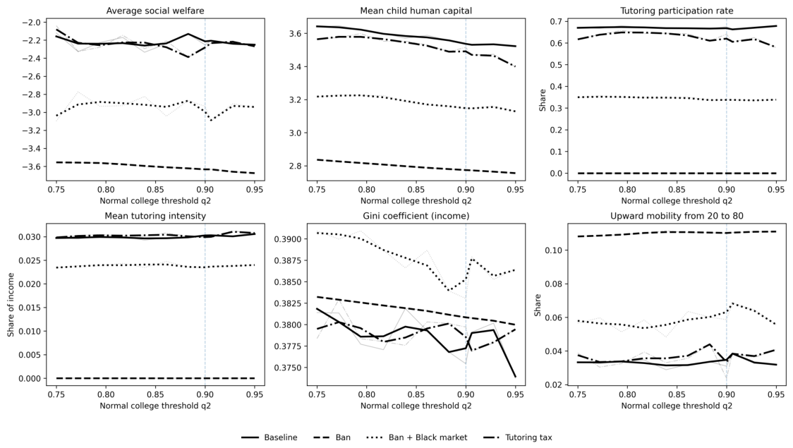
Figure 8 reports the corresponding results for variations in the selective college threshold q 2 . In contrast to q 1 , changes in q 2 have quantitatively smaller effects on aggregate outcomes. Welfare, child human capital, and tutoring behavior remain largely stable, while inequality declines as q 2 increases and other outcomes change little. The conditional policy ranking is again unchanged, indicating that the benchmark comparison is robust to alternative values of the upper admission threshold.

6.4. Admission Smoothness

Figure 9 reports the results when varying the admission smoothness parameter b, while holding all other parameters fixed. Higher b makes admission less sensitive to rank and therefore weakens tutoring incentives. As a result, mean child human capital, tutoring participation, and tutoring intensity all decline across policies, while upward mobility rises. Welfare increases with b, especially under the ban, because a smoother admission system reduces competition for rank. The effects on inequality are less monotonic, but they do not alter the qualitative comparison across policies. The conditional policy ranking remains unchanged throughout, with the welfare-selected tutoring tax performing best and the ban performing worst within the specified experiments.

7. Discussion and Limitations

The quantitative results should be interpreted as a mechanism-based policy comparison rather than a direct causal evaluation of a specific Chinese reform. The CFPS data discipline the benchmark economy, but several model parameters are mapped from reduced-form associations. In particular, the benchmark value of ω compares tutoring associations with exam-oriented subject tests and broader cognitive measures; tutoring expenditure remains endogenous, so this mapping is not a causal identification strategy. The intergenerational parameters θ and σ are anchored by the conditional parent–child relationship in completed education and its residual dispersion, and the education-track premia use conditional earnings differences. These mappings are informative but do not separately identify the corresponding structural technologies. The counterfactual and robustness exercises therefore assess how the main conclusions change when empirically less certain parameters are varied.
The policy comparison is also deliberately limited. The tutoring tax is selected to maximize average model utility over a fixed grid and is assumed to be collected effectively, whereas the prohibition experiments use fixed enforcement structures. A tax with evasion, an optimized enforcement policy, or a more flexible quantity regulation could produce a different ranking. In addition, the benchmark tutoring tax operates through both a price channel and a public-finance channel. Table 6 shows that, at the same tax rate, removing revenue recycling changes the model-implied CEV from positive to negative while leaving tutoring participation almost unchanged. The benchmark tax advantage therefore depends importantly on the assumed financing arrangement rather than on the tax instrument alone.
The black-market results are conditional on the assumed ordering of informal-access costs. Household resources already generate unequal tutoring demand, while the a j p parameters add a separate access advantage for more educated parents. These parameters are not direct estimates of underground tutoring prices or access costs. The results should therefore be read as showing how unequal informal access can affect policy incidence, with the sensitivity exercises indicating how strongly the outcomes depend on enforcement and access assumptions. Group-specific CEV measures are reported alongside aggregate welfare to make the distributional incidence explicit. As shown in the access-gap experiment, improvements in aggregate welfare can coexist with welfare losses for the bottom group when informal access becomes more unequal.
Finally, the model is partial equilibrium. Household tutoring and saving choices respond endogenously to policy, but wages, returns, aggregate labor demand, and other economy-wide feedbacks are held fixed. In a general-equilibrium setting, policy-induced changes in aggregate human capital could alter wages, skill premia, and the returns to education, which could in turn feed back into household investment incentives. The quantitative effects reported here should therefore be interpreted as operating through household education investment, admission competition, and intergenerational transmission within the modeled environment. The mechanisms may be relevant beyond China, particularly in education systems that share similar institutional features, such as high-stakes examination-based admissions, strong reliance on relative academic performance, and substantial household investment in supplementary education. In such settings, the qualitative policy trade-offs identified in the model may provide useful guidance, although the numerical effects should not be extrapolated directly without recalibration to local institutional and educational conditions. General-equilibrium labor-market responses, richer public-finance arrangements, and broader education reforms remain important extensions for future research.

8. Conclusions

This paper develops a quantitative framework to study how private tutoring regulation affects household behavior, human capital formation, inequality, and intergenerational mobility. The model combines heterogeneous households, intergenerational transmission, and endogenous ranking-based admission, while allowing tutoring to affect exam performance and productive skills differently.
In the benchmark calibration, a complete ban generates large model-implied welfare and human-capital losses, although it compresses educational differences and raises measured mobility. When enforcement is imperfect, informal tutoring preserves part of human-capital investment, but unequal access creates large differences in participation across parental education groups. A welfare-selected tutoring tax performs better than the prohibition experiments while keeping tutoring and human capital close to baseline levels. Its advantage, however, reflects both the tutoring-price channel and the replacement of part of the common public-education contribution.
The broader economic implication is that regulation of supplementary education can affect not only educational competition but also human-capital accumulation and the intergenerational distribution of opportunities. Regulation is more attractive when tutoring mainly improves relative rank and less attractive when it contributes strongly to productive skills, while policy outcomes also depend on enforcement and financing design. Because the productive contribution of tutoring is difficult to identify precisely, the pattern across alternative values of ω is more informative than the benchmark estimate alone. The results therefore support careful use of price and quantity instruments rather than a general claim that one instrument always dominates another. Although the numerical results are specific to the Chinese calibration, the mechanisms are relevant to other education systems with substantial household investment and competitive admission.
Future work could estimate the long-run productive effects of tutoring more directly, model tax evasion and endogenous enforcement, incorporate general-equilibrium labor-market responses, and compare tutoring regulation with reforms to examinations and admission rules. These extensions would help determine which mechanisms are quantitatively most important in particular education systems.


Supplementary Materials

The following supporting information can be downloaded at: https://www.mdpi.com/article/10.3390/economies14090415/s1.

Funding

This work was supported by JST SPRING, Grant Number JPMJSP2119.

Institutional Review Board Statement

Not applicable. This study uses de-identified secondary survey data and involves no direct interaction with human participants.

Informed Consent Statement

Not applicable.

Data Availability Statement

The China Family Panel Studies data used in this study are available from the Institute of Social Science Survey, Peking University, subject to its application and data-use conditions. The original CFPS microdata cannot be redistributed by the author. The code used for data construction, calibration, numerical simulations, and figure production is provided as Supplementary Materials.

Conflicts of Interest

The author declares no conflicts of interest.

Abbreviations

The following abbreviations are used in this manuscript:
CEVConsumption-equivalent variation
CFPSChina Family Panel Studies
CPIConsumer price index
OLGOverlapping generations

Appendix A. Model Details

Appendix A.1. Expected Child Consumption

The term c ˜ in the household problem denotes an expected lifetime-consumption index for the child. Given expected human capital E [ h ] , parents form expectations about the child’s future earnings and associated consumption choices. Let C ( h ) denote the policy mapping from adult human capital into the child’s two-period consumption index. Then,
c ˜ = E C ( h ) ,
where the expectation is taken over education outcomes and idiosyncratic shocks. In the numerical solution, C ( h ) is approximated by interpolating the consumption policy from the previous generation. This formulation is a parsimonious altruism channel and does not represent a direct transfer from the child to the parent.

Appendix A.2. Ranking and Endogenous Admission Mechanism

Admission probabilities depend on the child’s rank in the distribution of exam-relevant human capital. Let
κ = F ( h e x a m )
denote the child’s percentile rank, where F ( · ) is the cumulative distribution function of exam-relevant human capital.
The function F captures the ranking-based nature of admission: households map exam-relevant human capital into a relative position in the population, and admission depends on that position rather than on absolute scores. In the model, F is endogenous. Households take it as given when making decisions, but their decisions collectively determine the equilibrium distribution.
In the numerical solution, F is approximated by a reference distribution of exam-relevant human capital from the previous iteration. Given this reference distribution, households choose tutoring and savings, which generate a new distribution of exam outcomes. The reference distribution is then updated iteratively until convergence. At convergence, the distribution used by households is consistent with the distribution generated by optimal behavior.
Figure A1. College admission probabilities by percentile rank κ .
Economies 14 00415 g0a1
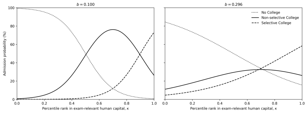
Figure A1 plots the admission probabilities for the three education tracks as functions of the child’s percentile rank κ in the distribution of exam-relevant human capital. The left panel shows the case with b = 0.1 , while the right panel uses the calibrated value b = 0.296 . In both cases, the probability of no college declines monotonically with rank, while the probability of selective-college admission rises monotonically. The probability of non-selective college is hump-shaped, since this track lies between the two admission thresholds and is therefore most likely for children in the intermediate range of the ranking distribution. The comparison also illustrates the role of b: a smaller value generates a steeper, more threshold-like admission schedule, whereas a larger value produces smoother transitions across education tracks.

Appendix A.3. Implied Admission Rates and Invariance Across Policies

Although admission is determined by ranking, aggregate track shares are mainly governed by the threshold parameters ( q 1 , q 2 ) . These thresholds determine the approximate fractions of students entering college and selective college. Policy changes therefore mainly affect which households are admitted to each track, rather than the total number of slots. Table A1 reports equilibrium track shares under different policy regimes.
Table A1. Education track shares across policies.
TrackBaselineBanBan + Black MarketTutoring Tax
No college0.4810.4700.4810.489
Non-selective college0.2640.2700.2640.256
Selective college0.2550.2610.2560.255

Appendix B. Welfare Measurement

Let U ¯ B denote average lifetime utility in the baseline economy and U ¯ P average lifetime utility under policy P. Because all utility components share the same CRRA curvature, the consumption-equivalent variation is computed as
CEV P = U ¯ P U ¯ B 1 1 ρ 1 .
The reported values multiply this expression by 100. The measure gives the uniform proportional change in the consumption index that reproduces the difference in average model utility. It includes parental consumption in both periods and the altruistic value of the child’s expected consumption. It is therefore not a comparison of tutoring expenditure alone.
For group-specific results, U ¯ B and U ¯ P are calculated within the same parental human-capital group. The CEV can differ from changes in mean child human capital or rank-based mobility because these statistics measure different components of the allocation. In particular, a policy can compress the outcome distribution and raise a relative mobility measure while lowering average lifetime utility.

Appendix C. Data Construction

This appendix describes the construction of the empirical dataset from the raw CFPS data. We use the 2010, 2012, 2014, 2016, 2018, 2020, and 2022 waves of the China Family Panel Studies (CFPS), combining information from the adult questionnaire, child questionnaire, family configuration module, and family economic module.
For each wave, we first merge the adult and child samples to construct a unified individual-level dataset and remove duplicate observations based on the individual identifier. We then merge household identifiers from the family configuration module and attach household-level economic variables from the family economic module. The resulting dataset is organized at the individual level with household-level information attached to each observation.
Because variable definitions differ across waves, we harmonize year-specific variable names into a common set of standardized variables. In particular, identifiers and key variables such as income, consumption, education expenditures, and test scores are converted into a consistent format. The harmonized wave-specific datasets are then stacked into a pooled repeated cross-section.
We also construct consistent indicators of participation in supplementary education across waves. The CFPS contains information on both out-of-school tutoring and school-based supplementary instruction, but the underlying survey questions vary across years. For each wave, we identify the relevant variables and recode them into binary indicators. Invalid and ambiguous responses are treated as missing.
Several cleaning procedures are applied before analysis. Key identifiers are converted to numeric format, non-numeric entries are treated as missing, and duplicate observations are removed. We further restrict the sample to observations with valid individual identifiers, household identifiers, geographic identifiers, and survey weights.
To make monetary variables comparable across time and regions, we use province-level consumer price index (CPI) data. The CPI series are reported as chain indices with the previous year equal to 100. For each province, we construct a price level index by chaining these growth rates over time and normalizing the index so that 2010 equals 100. Monetary variables are then converted into constant 2010 prices:
X i , t real = X i , t × 100 CPI p , t .
To account for household size, we use the OECD-modified equivalence scale:
eq_size = 1 + 0.5 × ( number of additional adults ) + 0.3 × ( number of children ) ,
where children are defined as individuals younger than 16, and individuals with missing age are treated as adults. Household-level monetary variables are divided by this scale. Combining the CPI adjustment and the equivalence-scale adjustment yields
X i , t real , eq = X i , t eq_size i , t × 100 CPI p , t .
Finally, all real, equivalized monetary variables are normalized by the weighted median of household wage income in 2010:
X i , t std = X i , t real , eq X ˜ 2010 .
The final dataset is a pooled repeated cross-section at the individual level. Each observation includes individual characteristics together with attached household-level variables, and all monetary variables are expressed in real, equivalized, and normalized units.

Appendix D. Calibration Details

This appendix describes how parameters are determined through externally fixed values, empirical estimates, and internal moment matching.

Appendix D.1. Details of the Externally Fixed and Benchmark Parameters

The externally fixed and benchmark parameters are described in Section 3.3 and reported in Table 1. These parameters are taken as given in the calibration.

Appendix D.2. Details of the Parameters Disciplined by Empirical Evidence

In this part, a set of model parameters is anchored by regression-based empirical relationships using the processed CFPS sample. These reduced-form relationships provide benchmark disciplines rather than causal identification of structural primitives.

Appendix D.2.1. Calibration of the Tutoring Efficiency Parameter ω

To construct a benchmark value for ω , we distinguish between exam-oriented outcomes and broader skill-oriented outcomes. Mathematics and word tests are used as proxies for exam-related academic performance, while digit-span and memory measures are used as proxies for broader cognitive skills. This distinction is empirical and approximate rather than structural: subject tests can also contain productive knowledge, and the broader cognitive measures do not span all dimensions of long-run productivity.
Each raw test measure is standardized within year–age cells. For exam-related outcomes, we use mathematics and word test scores. Let z i m a t h and z i w o r d denote the standardized values for child i. The exam index is
ExamIndex i = z i m a t h + z i w o r d 2 .
For skill-related outcomes, we use forward digit span, backward digit span, immediate memory, and delayed memory. Let z i f w , z i b w , z i i m m , and z i d e l denote the standardized values. The skill index is
SkillIndex i = z i f w + z i b w + z i i m m + z i d e l 4 .
The estimation sample is restricted to children aged 6–15 with non-missing outcomes and non-missing measures of school and tutoring expenditure. Denote school expenditure by e s and tutoring expenditure by p. Since both variables may be zero, we replace zeros with one tenth of the minimum strictly positive value in the corresponding sample before taking logs. The regressions are observational and do not solve the endogeneity of tutoring expenditure arising from selection into tutoring and correlated household resources:
log e s = log ( e s + ) , log p = log ( p + ) ,
where e s + and p + denote the adjusted expenditure variables.
We then estimate
ExamIndex i = α E + β s E log e s , i + β p E log p i + X i Γ E + ε i E ,
and
SkillIndex i = α S + β s S log e s , i + β p S log p i + X i Γ S + ε i S ,
where X i includes age, gender, urban status, and province fixed effects. The benchmark mapping is
ω = β ^ p S β ^ p E .
A lower value of ω implies that tutoring is more strongly associated with exam-related outcomes than with the broader skill proxy, while a higher value implies a stronger relative association with broader skill formation. Because the regressions are observational and the indices are imperfect proxies for the model’s two human-capital objects, the ratio is used as an empirical calibration device rather than as a causal estimate of the input-conversion technology. The benchmark value should therefore be read together with the full-range counterfactual and robustness exercises.

Appendix D.2.2. Calibration of Intergenerational Transmission Parameters θ and σ

The parameters governing intergenerational persistence are anchored using a standard parent–child regression based on completed educational attainment. We first construct parent–child pairs. For each child, the father’s identifier is used when available, and otherwise the mother’s identifier is used. The sample is restricted to individuals aged 25–35 so that educational attainment is largely completed. We then retain observations with non-missing child education, parental education, and strictly positive sampling weights.
Child and parent education are standardized within the estimation sample:
h ˜ i = h i h ¯ σ h , h ˜ p , i = h p , i h ¯ p σ h p .
We estimate
h ˜ i = α + θ h ˜ p , i + X i Γ + ε i ,
where X i includes gender, urban status, province fixed effects, and birth cohort, and the regression is weighted by the individual sampling weight. The persistence parameter is
θ = θ ^ ,
and the dispersion parameter is calibrated from the weighted standard deviation of the residuals:
σ = E w ε ^ i 2 .
Completed education is an equilibrium outcome that reflects inherited characteristics, family inputs, and institutions. The mapping therefore disciplines overall persistence and dispersion in the model; it does not isolate a biological or pre-investment endowment.

Appendix D.2.3. Calibration of College Returns Δj and Idiosyncratic Risk ηj

Individuals are classified into three education tracks according to highest educational attainment: high school or below ( j = 0 ), junior college ( j = 1 ), and bachelor’s degree or above ( j = 2 ). The estimation sample is restricted to employed individuals aged 25–55 with positive labor income and non-missing sampling weights. Labor income is measured in real, normalized terms, and log wages are defined as
log w i = log ( income i ) .
We estimate
log w i = α + β 1 1 { j = 1 } + β 2 1 { j = 2 } + X i Γ + ε i ,
where X i includes gender, a quadratic in age, urban status, province fixed effects, and year fixed effects. The college return parameters are
Δ 0 = 0 , Δ 1 = exp ( β ^ 1 ) 1 , Δ 2 = exp ( β ^ 2 ) 1 .
These conditional earnings differences may include selection into education. They are used as model-consistent earnings premia and are not interpreted as causal treatment effects of college attendance.
Let u i denote the residual from the wage regression. For each education track j, we compute the weighted residual standard deviation
σ u , j = E w [ u i 2 j ] .
This residual variation is mapped into the model’s idiosyncratic human capital shock by
σ η , j = ( 1 + Δ j ) σ u , j .

Appendix D.3. Details of the Internally Calibrated Parameters

The remaining parameters are calibrated within the model by matching a set of empirical target moments. This subsection first defines the target moments, then describes the calibration procedure.

Appendix D.3.1. Measurement of Calibration Targets

We construct empirical target moments from the CFPS data to discipline the internally calibrated parameters.
Saving Rate
The saving rate is defined as
Saving Rate = E y c y .
We restrict the sample to observations with positive income and consumption, exclude cases with consumption exceeding income, and trim extreme values. The resulting average saving rate is 0.422.
Life-Cycle Consumption Ratio
The life-cycle consumption ratio captures the difference in consumption between younger and older households. We compare average consumption between households with heads aged 35–39 and those with heads aged 40–45:
c c = exp E [ log c young ] E [ log c old ]
after excluding extreme values.
Education Expenditure Share
Education expenditure share is defined as the ratio of household education expenditure to household income. We focus on households with children aged 12–18 who are currently enrolled in school, trim the tails of both the income distribution and the expenditure-share distribution, and use the weighted median as the target moment.
Tutoring Participation and Intensity
Tutoring participation is the share of households that report positive tutoring expenditure or participation in tutoring classes. Tutoring intensity is
Intensity = E p y | p > 0 ,
where p denotes tutoring expenditure and y denotes household income. Extreme values are excluded, and the benchmark moment is taken from the 2020 wave for children aged 12–18.
Average Human Capital
Average human capital is proxied by labor income. Since model wages are proportional to human capital and the wage rate is normalized to one, we compute the trimmed mean of log income for employed individuals aged 22–60 with positive income and transform it back into levels.
Income Gradient in Tutoring Participation
Households are sorted by income after excluding extreme values, and the remaining sample is divided into five groups. The target moment is
Δ P T = 1 2 Part G 4 + Part G 5 1 2 Part G 1 + Part G 2 .
Admission Sensitivity
Admission sensitivity measures how strongly college access depends on relative academic performance. We construct an exam index by standardizing test scores within year–age cells and averaging across subjects, rank individuals by this index, and compute
Δ H L = Pr ( college exam Q 80 ) Pr ( college exam Q 20 ) .
College attendance is defined as at least junior college education.

Appendix D.3.2. Calibration Procedure

The internally calibrated parameters are obtained by matching model-generated moments to their empirical counterparts through numerical optimization. The procedure has three steps.
  • Step 1: Preference parameters
We first calibrate ( β , γ , ρ ) to match the saving rate, the education expenditure share, and the life-cycle consumption ratio. For any candidate parameter vector, the model is simulated under the baseline environment and the distance between model and data moments is measured by
L P = k m k model m k data σ k 2 ,
where σ k is a normalization parameter for moment k. We first perform a coarse grid search and then refine the estimates using local optimization.
  • Step 2: Education-related parameters
Conditional on the preference parameters, we jointly calibrate ( A , λ , μ , p 0 , b ) using tutoring participation, tutoring intensity, average human capital, admission sensitivity, and the income gradient in tutoring participation. The same quadratic loss function is used, together with a coarse grid search followed by local optimization.
  • Step 3: Full joint calibration
Finally, we jointly calibrate all parameters ( β , γ , ρ , A , λ , μ , p 0 , b ) . The first two steps are used to restrict the admissible parameter space to a neighborhood of the preliminary estimates. Within this restricted domain, we first conduct a random search to identify promising starting values, and then apply local optimization (Powell method with bound constraints) from multiple initial points. The solution with the lowest loss is selected.
  • Model simulation
For each evaluation of the loss function, the model is solved numerically by forward simulation. Given a candidate parameter vector, households choose tutoring expenditure and savings subject to the budget constraint, the distribution of human capital evolves across generations, and admission outcomes are determined by relative rank in exam performance. Iteration continues until the human-capital distribution converges.
This multi-step strategy improves numerical stability and reduces computational burden by narrowing the parameter space before the final joint search.

Appendix E. Numerical Method

This section describes the numerical procedure used to solve the model. 22 The solution combines forward simulation, policy function iteration, and fixed-point updating.
  • Step 1: Initialization
We initialize a cross-sectional distribution of households. Parental human capital is drawn from a log-normal distribution, households are assigned education types, and an initial reference distribution of exam performance is constructed.
  • Step 2: Household optimization
Given the current state distribution, households jointly choose consumption, savings, and private tutoring expenditure to maximize lifetime utility. Conditional on tutoring expenditure, optimal consumption and savings admit a closed-form solution from the Euler equation, reducing the problem to a one-dimensional search over tutoring expenditure.
For each household, utility is evaluated over a discretized tutoring grid. For each candidate tutoring level, we compute: (i) consumption and savings implied by the budget constraint; (ii) parental utility; (iii) exam performance and skill accumulation; (iv) admission probabilities based on relative rank; and (v) expected child utility using policy function interpolation. The tutoring level that maximizes expected utility is selected.
  • Step 3: Inner fixed point
Under the tutoring tax, an inner fixed-point problem is solved within each generation. Given household decisions, tutoring tax revenue is computed and the common contribution τ p is updated so that total public education spending e s remains fixed. This fixed point is solved by relaxation until convergence.
  • Step 4: Generation update
Given optimal household decisions, the next generation is formed. Child human capital is determined by inherited ability, educational investment, and stochastic shocks. Admission outcomes are then realized probabilistically.
  • Step 5: Distribution updating
The parental generation is replaced by realized child outcomes, and the reference distribution of exam performance is updated as a convex combination of the previous and newly generated distributions.
  • Step 6: Convergence
Steps 2–5 are repeated until the distribution of human capital converges. Convergence is assessed using the Wasserstein distance between successive distributions.
  • Step 7: Policy evaluation
The model is solved under the baseline, tutoring ban, ban with black market activity, and tutoring tax. For the tutoring tax policy, a grid search over rates from 0 to 0.30 in increments of 0.01 is used to select the value that maximizes average model utility. This optimization is specific to the tax experiment; the ban and black-market enforcement parameters are not jointly optimized.

Notes

1
Parents receive no direct material return from the child. The altruistic component is evaluated at expected child outcomes rather than separately integrating utility over every education and productivity realization. Appendix A gives the numerical mapping used to construct c ˜ .
2
In the simulation, ξ is log-normally distributed with mean one. It represents residual cross-sectional earnings heterogeneity rather than a transitory shock within the parent’s working life.
3
Public education and private tutoring are therefore imperfect substitutes. The same function is used in both human-capital channels so that their difference is summarized by a single tutoring-conversion wedge.
4
The use of ω p is a parsimonious reduced-form representation, not a claim that the underlying conversion technology is literally linear. Curvature in the effect of educational inputs is already captured by T ( · ) . Alternative mappings would require additional parameters that are not separately disciplined by the available data.
5
We model admission as a smooth function of percentile rank rather than as a deterministic quota rule. This preserves the central competitive feature of the system—higher relative rank raises admission chances—while allowing for uncertainty in the realized mapping from rank to placement. Such uncertainty may reflect exam noise, institutional frictions, or other non-score determinants of admission. The smooth formulation also avoids knife-edge discontinuities that would make household decisions and policy comparisons excessively sensitive to marginal rank changes. As b becomes small, the admission rule approaches a deterministic cutoff system. For college admission probabilities by percentile rank κ , see Figure A1 in Appendix A.2.
6
This ordering is intended to capture a qualitative access gradient rather than to estimate underground tutoring prices directly. More educated households may have better information, denser social networks, or greater ability to arrange small-scale private tutoring when formal providers are restricted. The benchmark values are therefore treated as scenario parameters, and Section 5 examines how the results change when both enforcement intensity and the access gap are varied. We refer to this residual informal sector as the “black market.”
7
The comparison is not a general ranking of optimal price and quantity instruments. The tax is assumed to be collected effectively, while informal networks are allowed under the imperfectly enforced ban. Similar networks could also facilitate tax evasion, and a more flexible quantity regulation could perform differently. We do not model those extensions because they would require additional enforcement parameters and policy experiments.
8
Details of the data construction are reported in Appendix C.
9
The 2010 and 2012 waves are excluded from this descriptive series because differences in survey definitions prevent the construction of directly comparable tutoring measures.
10
This implies that w = 1 corresponds to the typical level of household wage income in the data, and all other monetary variables are interpreted relative to this benchmark.
11
The parameters q 1 and q 2 do not represent the population shares of each education track. They are threshold values in the ranking-based admission mechanism, so higher values imply stricter admission criteria and lower implied enrollment rates.
12
Both proxy groups are imperfect. Subject tests can also capture productive knowledge, while memory and digit-span measures do not exhaust long-run productive skills. In addition, tutoring expenditure is endogenous because participation and spending reflect household characteristics and self-selection. The coefficient ratio is therefore used only to anchor a benchmark value and is not interpreted as a causal or structurally identified estimate of the tutoring-conversion technology. For this reason, the full range of ω is examined in Section 5.1 and Section 6.1.
13
Average human capital is measured as the mean realized child human capital in the model.
14
The model matches the income gradient in tutoring participation less precisely. In the data, participation rises moderately with income, whereas the model generates a somewhat steeper gradient. This reflects the difficulty of jointly matching both aggregate tutoring participation and its distribution across households within a parsimonious framework, since the transaction cost parameter p 0 affects both margins simultaneously.
15
To keep the main text focused on the economic results, the numerical solution is described in Appendix E.
16
Because zero is included in the grid, the selected tax cannot perform worse than the baseline according to the same welfare criterion. The tax result should therefore be interpreted as the best-performing tax experiment in the specified grid, not as the effect of an arbitrary tax rate.
17
The underlying concern is that much of private tutoring may be exam-oriented and improve test-taking performance more than long-run productive skills. Even when tutoring raises subject knowledge, exam-based learning need not fully coincide with productivity-relevant human capital.
18
Unless otherwise noted, all figures in the paper display smoothed series, while the underlying raw simulation results are shown as light lines. We adopt this presentation because the model contains several stochastic elements, which may introduce minor local fluctuations in some simulated outcome series. These fluctuations are generally limited and do not alter the overall pattern of the results. The smoothed lines are used only to improve visual clarity and highlight the underlying trend, while the raw lines remain available for reference.
19
In Figure 2, welfare rises with e s and then gradually converges toward zero, rather than exhibiting an inverted-U pattern. The reason is that public education spending is not purely distortionary in this framework. Although higher e s reduces private resources, it also directly raises human capital and partly substitutes for tutoring. The net effect therefore remains positive, but declines as public education increasingly replaces private tutoring.
20
The parameter a g a p is a scenario parameter that scales dispersion in black-market access across parental education types. A higher a g a p implies greater inequality in access to informal tutoring.
21
We do not impose an additional Rawlsian or inequality-averse social welfare criterion because doing so would require an extra normative choice over how welfare differences across groups should be weighted. Instead, we report group-specific CEV measures directly alongside aggregate welfare to make the distributional consequences transparent.
22
The computations are conducted using R 4.3.2, Python 3.13.5, NumPy 2.1.3, and CuPy 13.6.0.

References

  1. Abbott, B. (2022). Incomplete markets and parental investments in children. Review of Economic Dynamics, 44, 104–124. [Google Scholar] [CrossRef] [Scilit]
  2. Abbott, B., Gallipoli, G., Meghir, C., & Violante, G. L. (2019). Education policy and intergenerational transfers in equilibrium. Journal of Political Economy, 127(6), 2569–2624. [Google Scholar] [CrossRef] [Scilit]
  3. Abdulla, K. (2023). New evidence on the role of human capital in economic development. Applied Economics, 55(10), 1062–1073. [Google Scholar] [CrossRef] [Scilit]
  4. Bray, M. (2006). Private supplementary tutoring: Comparative perspectives on patterns and implications. Compare, 36(4), 515–530. [Google Scholar] [CrossRef] [Scilit]
  5. Bray, M. (2024). Still in need of confronting: Shadow education and its implications in the sustainable development goals. International Journal of Educational Development, 104, 102967. [Google Scholar] [CrossRef] [Scilit]
  6. Buchmann, C., Condron, D. J., & Roscigno, V. J. (2010). Shadow education, American style: Test preparation, the SAT, and college enrollment. Social Forces, 89(2), 435–461. [Google Scholar] [CrossRef] [Scilit]
  7. Caucutt, E. M., & Lochner, L. (2020). Early and late human capital investments, borrowing constraints, and the family. Journal of Political Economy, 128(3), 1065–1147. [Google Scholar] [CrossRef] [Scilit]
  8. Dang, H.-A., & Rogers, F. H. (2008). The growing phenomenon of private tutoring: Does it deepen human capital, widen inequalities, or waste resources? The World Bank Research Observer, 23(2), 161–200. [Google Scholar] [CrossRef] [Scilit]
  9. Gu, S., & Zhang, L. (2024, June 13–16). The macroeconomic consequences of competition for college admissions. 2024 North America Summer Meeting of the Econometric Society, Nashville, TV, USA. [Google Scholar]
  10. Guill, K., & Lintorf, K. (2019). Private tutoring when stakes are high: Insights from the transition from primary to secondary school in Germany. International Journal of Educational Development, 65, 172–182. [Google Scholar] [CrossRef] [Scilit]
  11. Guo, Y., Chen, Q., Zhai, S., & Pei, C. (2020). Does private tutoring improve student learning in China? Evidence from the China education panel survey. Asia & the Pacific Policy Studies, 7(3), 322–343. [Google Scholar] [CrossRef] [Scilit]
  12. Hajar, A., & Karakus, M. (2022). A bibliometric mapping of shadow education research: Achievements, limitations, and the future. Asia Pacific Education Review, 23(2), 341–359, (Correction in 2023, Asia Pacific Education Review, 27, 399). [Google Scholar] [CrossRef] [Scilit]
  13. Karakus, M., Tlessov, A., Hajar, A., & Courtney, M. (2024). Illuminating the shadows: The role of private supplementary tutoring on student math performance in PISA 2022. Large-Scale Assessments in Education, 12(1), 42. [Google Scholar] [CrossRef] [Scilit]
  14. Kim, S., & Lee, J.-H. (2010). Private tutoring and demand for education in South Korea. Economic Development and Cultural Change, 58(2), 259–296. [Google Scholar] [CrossRef] [Scilit]
  15. Kim, S., Tertilt, M., & Yum, M. (2024). Status externalities in education and low birth rates in Korea. American Economic Review, 114(6), 1576–1611. [Google Scholar] [CrossRef] [Scilit]
  16. Kim, T., Jang, H., & Kim, J. (2022). Do peers affect private tutoring engagement in Korea? Evidence from a quasi-experimental approach. Asia Pacific Education Review, 23(2), 271–283. [Google Scholar] [CrossRef] [Scilit]
  17. Kuan, P.-Y. (2011). Effects of cram schooling on mathematics performance: Evidence from junior high students in Taiwan. Comparative Education Review, 55(3), 342–368. [Google Scholar] [CrossRef] [Scilit]
  18. Lee, J. C., Quadlin, N., & Ambriz, D. (2023). Shadow education, pandemic style: Social class, race, and supplemental education during COVID-19. Research in Social Stratification and Mobility, 83, 100755. [Google Scholar] [CrossRef] [Scilit] [PubMed]
  19. Lee, S. Y., & Seshadri, A. (2019). On the intergenerational transmission of economic status. Journal of Political Economy, 127(2), 855–921. [Google Scholar] [CrossRef] [Scilit] [PubMed]
  20. Liu, J., & Bray, M. (2017). Determinants of demand for private supplementary tutoring in China: Findings from a national survey. Education Economics, 25(2), 205–218. [Google Scholar] [CrossRef] [Scilit]
  21. Matsuoka, R. (2018). Inequality in shadow education participation in an egalitarian compulsory education system. Comparative Education Review, 62(4), 565–586. [Google Scholar] [CrossRef] [Scilit] [PubMed]
  22. Pan, Z., Lien, D., & Wang, H. (2022). Peer effects and shadow education. Economic Modelling, 111, 105822. [Google Scholar] [CrossRef] [Scilit]
  23. Ramey, G., & Ramey, V. A. (2010). The rug rat race. In Brookings papers on economic activity (pp. 129–176). Brookings Institution Press. [Google Scholar]
  24. Stevenson, D. L., & Baker, D. P. (1992). Shadow education and allocation in formal schooling: Transition to university in Japan. American Journal of Sociology, 97(6), 1639–1657. [Google Scholar] [CrossRef] [Scilit] [PubMed]
  25. Sun, L., Shafiq, M. N., McClure, M., & Guo, S. (2020). Are there educational and psychological benefits from private supplementary tutoring in mainland China? Evidence from the China education panel survey, 2013–15. International Journal of Educational Development, 72, 102144. [Google Scholar] [CrossRef] [Scilit]
  26. Zhang, W., & Bray, M. (2020). Comparative research on shadow education: Achievements, challenges, and the agenda ahead. European Journal of Education, 55(3), 322–341. [Google Scholar] [CrossRef] [Scilit]
  27. Zhang, Y. (2013). Does private tutoring improve students’ national college entrance examination performance? A case study from Jinan, China. Economics of Education Review, 32, 1–28. [Google Scholar] [CrossRef] [Scilit]
  28. Zheng, X., Wang, C., Shen, Z., & Fang, X. (2020). Associations of private tutoring with Chinese students’ academic achievement, emotional well-being, and parent–child relationship. Children and Youth Services Review, 112, 104934. [Google Scholar] [CrossRef] [Scilit]
  29. Zwier, D., Geven, S., & van de Werfhorst, H. G. (2020). Social inequality in shadow education: The role of high-stakes testing. International Journal of Comparative Sociology, 61(6), 412–440. [Google Scholar] [CrossRef] [Scilit]
Figure 1. Private tutoring participation and intensity in the CFPS, 2014–2022. Notes: The sample includes children aged 12–18 in households with positive income. The left panel reports the share participating in private tutoring. The right panel reports tutoring expenditure as a share of household income conditional on participation.
Economies 14 00415 g001
Figure 2. Effects of public education spending. Notes: This figure shows how key outcomes vary with public education spending e s under different policy regimes. The fitted curve is obtained using nonparametric smoothing, while the light line shows raw simulation results.The vertical dashed line indicates the calibrated value.
Economies 14 00415 g002
Figure 3. Black-market enforcement intensity. Notes: This figure shows how outcomes vary with enforcement intensity φ . The fitted curve is obtained using nonparametric smoothing, while the light line shows raw simulation results.
Economies 14 00415 g003
Figure 4. Robustness test of the relative effectiveness of tutoring ( ω ). Notes: The figure shows robustness results with respect to the relative effectiveness of tutoring ω . The fitted curve is obtained using nonparametric smoothing, while the light line shows raw simulation results. The vertical dashed line indicates the calibrated value.
Economies 14 00415 g004
Figure 5. Robustness test of intergenerational persistence ( θ ). Notes: The lines connect raw simulation results. The vertical dashed line indicates the calibrated value.
Economies 14 00415 g005
Figure 6. Robustness test of inheritance-shock dispersion ( σ ). Notes: The lines connect raw simulation results. The vertical dashed line indicates the calibrated value.
Economies 14 00415 g006
Figure 7. Robustness test of non-selective college threshold ( q 1 ). Notes: The figure shows robustness results with respect to the non-selective college admission threshold q 1 . The fitted curve is obtained using nonparametric smoothing, while the light line shows raw simulation results. The vertical dashed line indicates the calibrated value.
Economies 14 00415 g007
Figure 8. Robustness test of selective college threshold ( q 2 ). Notes: The figure shows robustness results with respect to the selective college admission threshold q 2 . The fitted curve is obtained using nonparametric smoothing, while the light line shows raw simulation results. The vertical dashed line indicates the calibrated value.
Economies 14 00415 g008
Figure 9. Robustness test of admission smoothness (b). Notes: The figure shows robustness results with respect to the admission smoothness parameter b. The fitted curve is obtained using nonparametric smoothing, while the light line shows raw simulation results. The vertical dashed line indicates the calibrated value.
Economies 14 00415 g009
Table 1. Externally Fixed and Benchmark Parameters.
ParameterDescriptionValueSource
wWage rate1Normalization
r δ Net return on savings0.02Government bond yields
e s Public education expenditure0.1826CFPS 2016–2022
q 1 Admission threshold (non-selective college)0.5Benchmark value
q 2 Admission threshold (selective college)0.9Benchmark value
φ Enforcement intensity3.5Scenario value
a 0 Informal-access cost of type 0 parents1Scenario value
a 1 Informal-access cost of type 1 parents0.8Scenario value
a 2 Informal-access cost of type 2 parents0.6Scenario value
Notes: This table reports parameters fixed by normalization, direct measurement, or benchmark scenario assumptions.
Table 2. Parameters disciplined by estimation.
ParameterDescriptionValueEmpirical Discipline
ω Tutoring conversion rate in skill formation0.308Relative tutoring effects across exam- and skill-related outcomes
θ Intergenerational persistence0.189Parent–child regression
σ Dispersion of inheritance shocks0.653Residual variation in intergenerational transmission
Δ 0 Non-college return0Normalization
Δ 1 Earnings premium: non-selective college0.714Wage regression
Δ 2 Earnings premium: selective college0.974Wage regression
η 0 Shock dispersion (non-college)0.887Within-group residual variation
η 1 Shock dispersion (non-selective college)1.320Within-group residual variation
η 2 Shock dispersion (selective college)1.470Within-group residual variation
Notes: This table reports benchmark parameter values disciplined by reduced-form empirical relationships. The mappings are not interpreted as causal identification of structural primitives.
Table 3. Internally calibrated parameters and targeted moments.
ParameterDescriptionValueTarget MomentDataModel
β Discount factor0.844Saving rate0.4220.420
γ Parental altruism0.627Education share0.1060.119
ρ CRRA coefficient2.388 c / c 1.0591.065
AUnified scale in T ( e s , x ) 16.138Mean child human capital3.4933.537
λ Weight on school input in T ( e s , x ) 0.613Tutoring participation rate0.6780.679
μ Elasticity parameter in T ( e s , x ) 0.519Tutoring intensity0.0350.031
p 0 Tutoring transaction cost0.873Income gradient in tutoring participation0.2650.400
bAdmission smoothness0.296Admission sensitivity0.5880.563
Notes: This table reports parameters calibrated to match model-generated moments to their empirical counterparts. CRRA denotes the constant relative risk aversion.
Table 4. Standardized income distribution: data vs. model.
P10P20P30P40P50P60P70P80P90
Data−0.991−0.821−0.654−0.476−0.276−0.0460.2480.6661.415
Model−1.023−0.824−0.648−0.463−0.251−0.0010.3180.7281.375
Notes: Income is measured in standardized units. In the data, all monetary variables are first converted into real terms, equivalized, and normalized by the weighted median of household wage income in 2010. Model income is expressed in the same unit.
Table 5. Calibrated benchmark: overall policy comparison.
VariableBaselineBanBan + Black MarketTutoring Tax
CEV0.000−30.141−16.5871.292
Mean child human capital3.5372.7743.1533.522
Tutoring participation rate0.6790.0000.3420.661
Mean tutoring intensity0.0310.0000.0240.031
Gini coefficient (income)0.3750.3810.3840.375
Upward mobility from 20 to 800.0350.1100.0580.030
Notes: This table reports aggregate outcomes under different policy regimes at calibrated parameters. CEV denotes the percentage consumption-equivalent variation implied by average model utility relative to the baseline. Upward mobility measures the probability that a child from the bottom 20% of the parental human-capital distribution reaches the top 20% of the child human-capital distribution in the next generation.
Table 6. Decomposing the effects of the tutoring tax.
VariableBaselineTax with RecyclingTax Without Recycling
CEV0.0001.292−2.194
Mean child human capital3.5373.5223.542
Tutoring participation rate0.6790.6610.660
Tutoring tax rate0.0000.0600.060
Tutoring tax revenue0.0000.0070.007
Household public-education contribution0.1830.1760.183
Notes: The no-recycling counterfactual imposes the same tutoring-tax rate as the benchmark tax but does not use the resulting revenue to reduce the common household contribution to public education. Welfare calculations follow the same sample definition as the benchmark results.
Table 7. Calibrated benchmark: cross-group comparison.
PolicyBottom 30%Middle 40%Top 30%
CEVBaseline0.0000.0000.000
Ban−37.298−23.521−25.906
Ban + Black market−11.239−16.321−14.231
Tutoring tax10.794−1.514−0.508
Child human capitalBaseline2.1213.3285.085
Ban2.2032.6023.473
Ban + Black market2.1752.7714.486
Tutoring tax2.1023.3155.067
Participation rateBaseline0.1300.8150.989
Ban0.0000.0000.000
Ban + Black market0.0040.2050.809
Tutoring tax0.1180.7800.988
Reach top 20%Baseline0.0400.1470.414
Ban0.1140.1640.318
Ban + Black market0.0610.1410.395
Tutoring tax0.0390.1500.410
Notes: This table reports outcomes under different policy regimes across household groups defined by parental human capital. Reach top 20% measures the probability that a child from a given parental human-capital group enters the top 20% of the child outcome distribution.
Table 8. Cross-group comparison at ω = 0 , calibrated ω = 0.308 , and ω = 1 .
PolicyBottom 30%Middle 40%Top 30%
ω 0Calib.10Calib.10Calib.1
CEV
Baseline0.0000.0000.0000.0000.0000.0000.0000.0000.000
Ban−0.464−37.298−64.5372.248−23.521−47.356−1.794−25.906−48.249
Ban + Black market3.346−11.239−45.5620.573−16.321−31.211−1.755−14.231−23.135
Tutoring tax6.16310.7940.0002.279−1.5140.000−1.527−0.5080.000
Mean child human capital
Baseline2.0612.1212.7542.5133.3284.6953.5275.0857.483
Ban2.1762.2032.1762.5602.6022.5603.4743.4733.474
Ban + Black market2.1542.1752.0952.5702.7713.3503.4734.4866.054
Tutoring tax2.1092.1022.7542.5683.3154.6953.5425.0677.483
Tutoring participation rate
Baseline0.0230.1300.4420.4390.8150.9650.9020.9890.999
Ban0.0000.0000.0000.0000.0000.0000.0000.0000.000
Ban + Black market0.0000.0040.0100.0920.2050.3930.5560.8090.937
Tutoring tax0.0140.1180.4420.3560.7800.9650.8470.9880.999
Reach top 20%
Baseline0.0960.0400.0220.1570.1470.1280.3420.4140.465
Ban0.1120.1140.1120.1660.1640.1660.3160.3180.316
Ban + Black market0.1030.0610.0210.1660.1410.1200.3250.3950.463
Tutoring tax0.1000.0390.0220.1610.1500.1280.3350.4100.465
Notes: This table compares outcomes across parent human capital groups under three values of ω . The parameter ω governs the effectiveness of private tutoring in skill formation.
Table 9. Ban with black market results at alternative values of a gap .
OverallBottom 30%Middle 40%Top 30%
a gap 0Calib.1.50Calib.1.50Calib.1.50Calib.1.5
CEV−20.69−16.59−14.50−22.38−11.24−13.81−17.53−16.32−14.73−15.31−14.23−11.01
Child HC3.103.153.192.182.182.162.652.772.774.464.494.60
Part. rate0.290.340.370.000.000.000.160.210.240.700.810.85
Reach top 20% 0.080.060.060.120.140.130.410.400.40
Notes: This table reports outcomes under the ban-with-black-market regime for different values of a g a p . The probability of reaching the top 20% is not reported for the overall population, as this measure is defined only for group-specific comparisons. The parameter a g a p maps into the type-specific access parameters a j . When a g a p = 0 , access is equal across groups ( a j = 1 for all j). At the calibrated value, access is given by ( 1 , 0.8 , 0.6 ) , while a g a p = 1.5 corresponds to ( 1 , 0.7 , 0.4 ) , reflecting greater inequality in access to informal tutoring.
Disclaimer/Publisher’s Note: The statements, opinions and data contained in all publications are solely those of the individual author(s) and contributor(s) and not of MDPI and/or the editor(s). MDPI and/or the editor(s) disclaim responsibility for any injury to people or property resulting from any ideas, methods, instructions or products referred to in the content.