
Convergence of the Agricultural Share in GDP in Central and Eastern Europe: A Statistical and Econometric Analysis


Abstract
1. Introduction
2. Literature Review
2.1. Agricultural Share in GDP
2.1.1. Structural Transformation and the Relative Decline of Agriculture
2.1.2. Measurement Boundaries: Primary Agriculture Versus the Agribusiness System
2.1.3. The Persistent Strategic Role of Agriculture in Transition Economies
2.1.4. Value-Chain Dynamics and the Composition of Agricultural Output
2.1.5. Macro-Institutional and Spatial Determinants of Agricultural Decline
2.2. Economic Convergence Theory
2.2.1. Theoretical Foundations of Convergence
2.2.2. Divergence Between β- and σ-Convergence
2.2.3. Convergence at the National Versus Regional Level
2.2.4. The Domain-Specific Nature of Convergence
2.2.5. Empirical Evidence on Convergence in the Agricultural Sector
2.3. Research Gaps
3. Research Methodology
3.1. Data
3.2. Methods
4. Results
4.1. Statistical Analysis
σ-Convergence and β-Convergence
- -
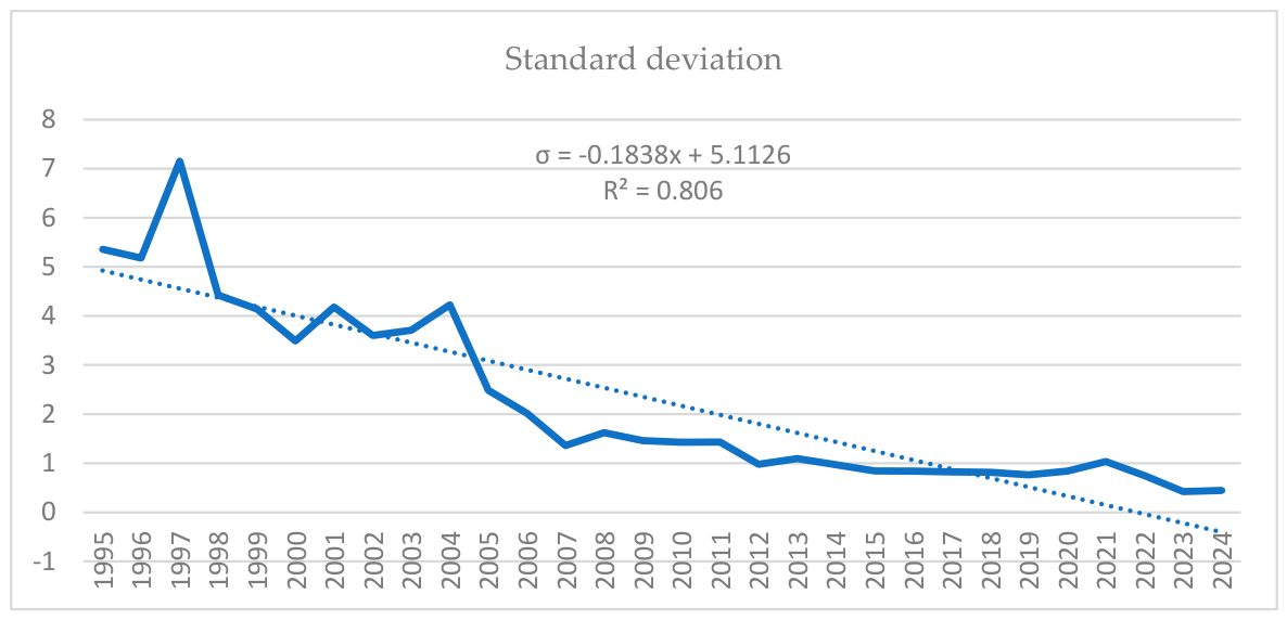
- σ-convergence shows that the dispersion between countries has reduced over the period analyzed (1995–2024), with the standard deviation decreasing from approximately 5.36 to 0.45.
- -
- β-convergence shows that countries with higher initial agricultural shares have experienced faster reductions, which is consistent with the process of structural convergence.
4.2. ARIMA Forecasting
4.2.1. Romania
4.2.2. Bulgaria
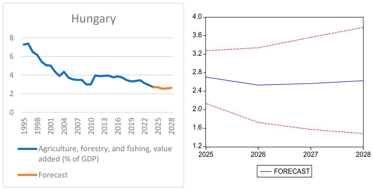
4.2.3. Hungary
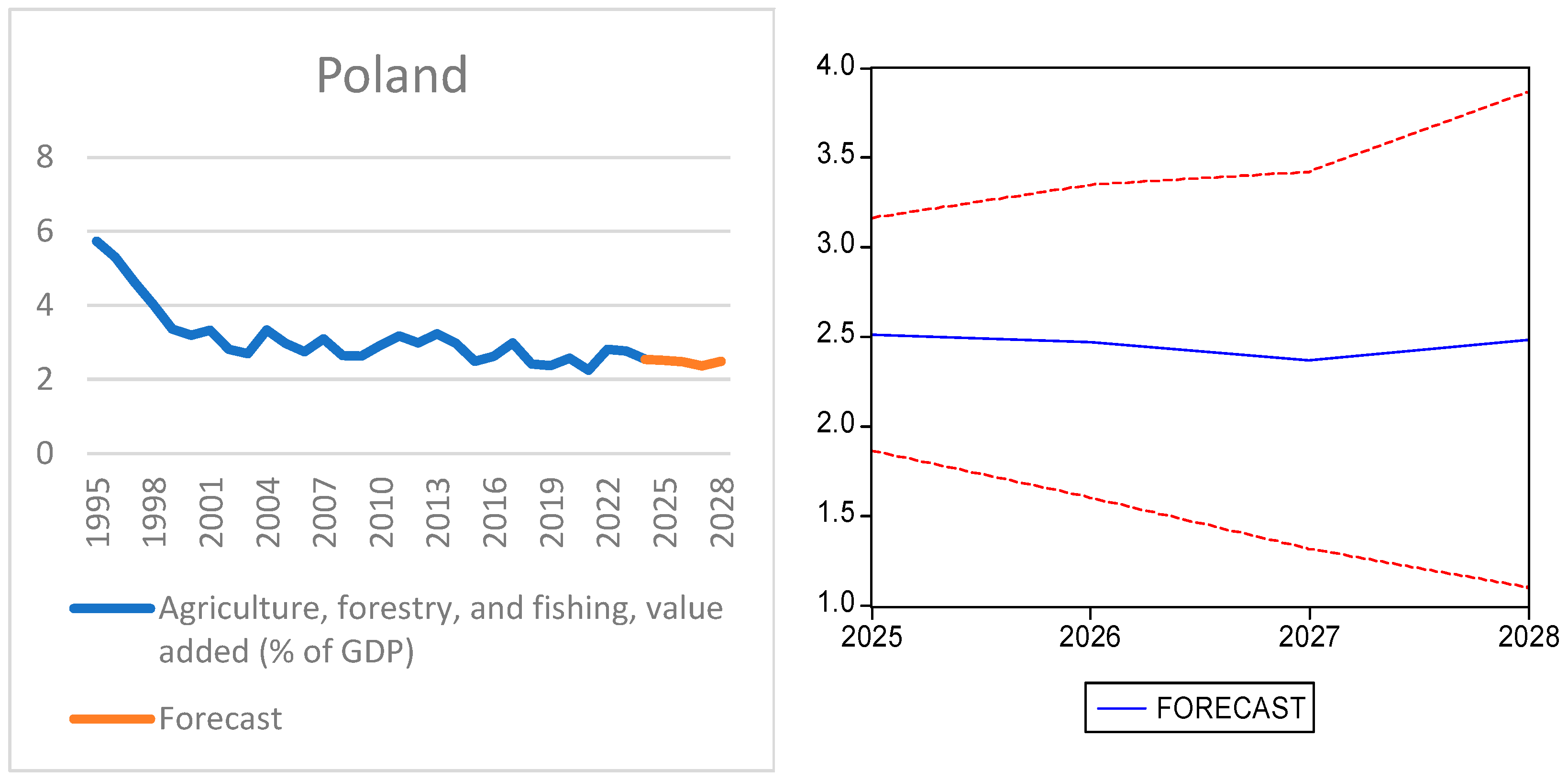
4.2.4. Poland
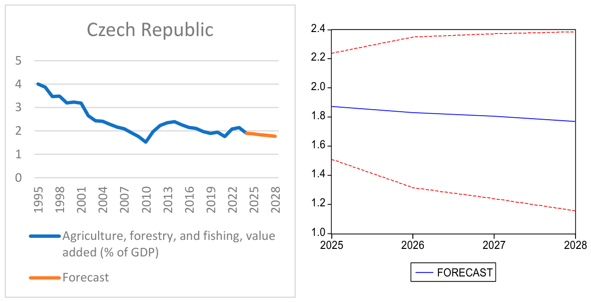
4.2.5. The Czech Republic
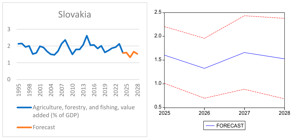
4.2.6. Slovakia
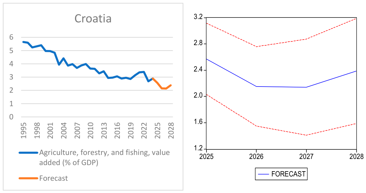
4.2.7. Croatia
5. Discussion
6. Conclusions
Author Contributions
Funding
Institutional Review Board Statement
Informed Consent Statement
Data Availability Statement
Conflicts of Interest
Appendix A

| Autocorrelation | Partial Correlation | AC | PAC | Q-Stat | Prob | |
|---|---|---|---|---|---|---|
| . **| . | | . **| . | | 1 | −0.249 | −0.249 | 1.9867 | 0.159 |
| . |* . | | . |* . | | 2 | 0.151 | 0.095 | 2.7464 | 0.253 |
| . *| . | | . | . | | 3 | −0.077 | −0.021 | 2.9537 | 0.399 |
| . **| . | | . **| . | | 4 | −0.235 | −0.292 | 4.9408 | 0.293 |
| . |* . | | . |* . | | 5 | 0.187 | 0.097 | 6.2514 | 0.283 |
| . **| . | | . *| . | | 6 | −0.244 | −0.142 | 8.5780 | 0.199 |
| . |*** | | . |*** | | 7 | 0.433 | 0.339 | 16.231 | 0.023 |
| . | . | | . |* . | | 8 | −0.054 | 0.104 | 16.353 | 0.038 |
| . | . | | . | . | | 9 | 0.010 | −0.036 | 16.358 | 0.060 |
| . |* . | | . | . | | 10 | 0.069 | 0.028 | 16.585 | 0.084 |
| . *| . | | . | . | | 11 | −0.175 | 0.057 | 18.116 | 0.079 |
| . | . | | . *| . | | 12 | 0.066 | −0.081 | 18.343 | 0.106 |
| Variable | Coefficient | Std. Error | t-Statistic | Prob. |
|---|---|---|---|---|
| C | −0.212289 | 0.300808 | −0.705729 | 0.4881 |
| AR(5) | 0.327408 | 0.116259 | 2.816185 | 0.0103 |
| MA(7) | 0.957846 | 0.029826 | 32.11464 | 0.0000 |
| R-squared | 0.837284 | Mean dependent var | −0.335103 | |
| Adjusted R-squared | 0.821787 | S.D. dependent var | 1.279771 | |
| S.E. of regression | 0.540259 | Akaike info criterion | 1.722933 | |
| Sum squared resid | 6.129477 | Schwarz criterion | 1.870189 | |
| Log likelihood | −17.67519 | F-statistic | 54.02945 | |
| Durbin-Watson stat | 2.793782 | Prob(F-statistic) | 0.000000 | |
| Inverted AR Roots | 0.80 | 0.25 − 0.76i | 0.25 + 0.76i | −0.65 − 0.47i |
| −0.65 + 0.47i | ||||
| Inverted MA Roots | 0.90 + 0.43i | 0.90 − 0.43i | 0.22 − 0.97i | 0.22 + 0.97i |
| −0.62 − 0.78i | −0.62 + 0.78i | −0.99 | ||
| Breusch-Godfrey Serial Correlation LM Test: | ||||
| F-statistic | 2.197390 | Probability | 0.138525 | |
| ARCH Test: | ||||
| F-statistic | 0.690308 | Probability | 0.415406 | |
| Sample: 1998–2024 | ||||||
|---|---|---|---|---|---|---|
| Included Observations: 26 | ||||||
| Autocorrelation | Partial Correlation | AC | PAC | Q-Stat | Prob | |
| . *| . | | . *| . | | 1 | −0.064 | −0.064 | 0.1198 | 0.729 |
| . | . | | . | . | | 2 | 0.052 | 0.048 | 0.2018 | 0.904 |
| . |**. | | . |**. | | 3 | 0.204 | 0.212 | 1.5215 | 0.677 |
| . | . | | . |* . | | 4 | 0.065 | 0.095 | 1.6616 | 0.798 |
| . |* . | | . |* . | | 5 | 0.128 | 0.125 | 2.2315 | 0.816 |
| . | . | | . | . | | 6 | 0.024 | −0.006 | 2.2522 | 0.895 |
| . |* . | | . | . | | 7 | 0.073 | 0.032 | 2.4587 | 0.930 |
| . *| . | | . **| . | | 8 | −0.169 | −0.236 | 3.6104 | 0.890 |
| . |* . | | . |* . | | 9 | 0.139 | 0.083 | 4.4415 | 0.880 |
| . | . | | . *| . | | 10 | −0.044 | −0.062 | 4.5302 | 0.920 |
| . **| . | | . *| . | | 11 | −0.194 | −0.152 | 6.3486 | 0.849 |
| . *| . | | . **| . | | 12 | −0.162 | −0.254 | 7.7150 | 0.807 |
| Variable | Coefficient | Std. Error | t-Statistic | Prob. |
|---|---|---|---|---|
| C | −0.187645 | 0.112840 | −1.662924 | 0.1112 |
| AR(2) | 0.639488 | 0.131603 | 4.859230 | 0.0001 |
| MA(2) | −0.930384 | 0.037211 | −25.00297 | 0.0000 |
| R-squared | 0.223218 | Mean dependent var | −0.359143 | |
| Adjusted R-squared | 0.149239 | S.D. dependent var | 0.707547 | |
| S.E. of regression | 0.652618 | Akaike info criterion | 2.100818 | |
| Sum squared resid | 8.944110 | Schwarz criterion | 2.248075 | |
| Log likelihood | −22.20982 | F-statistic | 3.017313 | |
| Durbin-Watson stat | 2.298349 | Prob(F-statistic) | 0.070492 | |
| Inverted AR Roots | 0.80 | −0.80 | ||
| Inverted MA Roots | 0.96 | −0.96 | ||
| Breusch-Godfrey Serial Correlation LM Test: | ||||
| F-statistic | 0.571836 | Probability | 0.573908 | |
| ARCH Test: | ||||
| F-statistic | 0.898219 | Probability | 0.354039 | |
| Autocorrelation | Partial Correlation | AC | PAC | Q-Stat | Prob | |
|---|---|---|---|---|---|---|
| . | . | | . | . | | 1 | 0.000 | 0.000 | 3 × 10⁻⁶ | 0.999 |
| . | . | | . | . | | 2 | 0.001 | 0.001 | 2 × 10⁻⁵ | 1.000 |
| . |**. | | . |**. | | 3 | 0.291 | 0.291 | 2.9263 | 0.403 |
| . |* . | | . |* . | | 4 | 0.076 | 0.083 | 3.1326 | 0.536 |
| . | . | | . | . | | 5 | 0.031 | 0.035 | 3.1675 | 0.674 |
| . | . | | . *| . | | 6 | 0.000 | −0.091 | 3.1675 | 0.788 |
| . | . | | . | . | | 7 | 0.050 | 0.002 | 3.2692 | 0.859 |
| . | . | | . | . | | 8 | −0.016 | −0.044 | 3.2799 | 0.916 |
| . *| . | | . *| . | | 9 | −0.108 | −0.097 | 3.8005 | 0.924 |
| . |* . | | . |* . | | 10 | 0.124 | 0.122 | 4.5290 | 0.920 |
| . **| . | | .**| . | | 11 | −0.238 | −0.248 | 7.3589 | 0.769 |
| . *| . | | . *| . | | 12 | −0.128 | −0.078 | 8.2211 | 0.768 |
| Variable | Coefficient | Std. Error | t-Statistic | Prob. |
|---|---|---|---|---|
| C | −0.011719 | 0.075746 | −0.154714 | 0.8785 |
| AR(5) | 0.456668 | 0.172944 | 2.640553 | 0.0153 |
| MA(5) | −0.880006 | 0.058159 | −15.13109 | 0.0000 |
| R-squared | 0.353659 | Mean dependent var | −0.098110 | |
| Adjusted R-squared | 0.292102 | S.D. dependent var | 0.335908 | |
| S.E. of regression | 0.282621 | Akaike info criterion | 0.427051 | |
| Sum squared resid | 1.677372 | Schwarz criterion | 0.574308 | |
| Log likelihood | −2.124616 | F-statistic | 5.745286 | |
| Durbin-Watson stat | 1.867423 | Prob(F-statistic) | 0.010229 | |
| Inverted AR Roots | 0.85 | 0.26 − 0.81i | 0.26 + 0.81i | −0.69 + 0.50i |
| −0.69 − 0.50i | ||||
| Inverted MA Roots | 0.97 | 0.30 + 0.93i | 0.30 − 0.93i | −0.79 − 0.57i |
| −0.79 + 0.57i | ||||
| Breusch-Godfrey Serial Correlation LM Test: | ||||
| F-statistic | 0.839786 | Probability | 0.447213 | |
| ARCH Test: | ||||
| F-statistic | 0.209949 | Probability | 0.651514 | |
| Autocorrelation | Partial Correlation | AC | PAC | Q-Stat | Prob | |
|---|---|---|---|---|---|---|
| . | . | | . | . | | 1 | 0.003 | 0.003 | 0.0002 | 0.988 |
| . *| . | | . *| . | | 2 | −0.129 | −0.129 | 0.5557 | 0.757 |
| . |*** | | . |*** | | 3 | 0.447 | 0.455 | 7.4582 | 0.059 |
| . *| . | | . **| . | | 4 | −0.115 | −0.206 | 7.9337 | 0.094 |
| . **| . | | . *| . | | 5 | −0.221 | −0.096 | 9.7638 | 0.082 |
| . |**. | | . |* . | | 6 | 0.302 | 0.125 | 13.327 | 0.038 |
| . | . | | . | . | | 7 | −0.046 | −0.001 | 13.414 | 0.063 |
| . **| . | | . *| . | | 8 | −0.303 | −0.186 | 17.352 | 0.027 |
| . |* . | | . | . | | 9 | 0.188 | 0.031 | 18.947 | 0.026 |
| . |* . | | . |* . | | 10 | 0.094 | 0.130 | 19.362 | 0.036 |
| . **| . | | . | . | | 11 | −0.230 | −0.027 | 22.005 | 0.024 |
| . | . | | . *| . | | 12 | 0.035 | −0.163 | 22.069 | 0.037 |
| Variable | Coefficient | Std. Error | t-Statistic | Prob. |
|---|---|---|---|---|
| C | 0.009617 | 0.172381 | 0.055787 | 0.9560 |
| AR(3) | 0.442952 | 0.200200 | 2.212550 | 0.0371 |
| MA(7) | 0.775005 | 0.097180 | 7.974923 | 0.0000 |
| R-squared | 0.434297 | Mean dependent var | −0.056848 | |
| Adjusted R-squared | 0.385106 | S.D. dependent var | 0.353956 | |
| S.E. of regression | 0.277555 | Akaike info criterion | 0.382575 | |
| Sum squared resid | 1.771851 | Schwarz criterion | 0.527740 | |
| Log likelihood | −1.973470 | F-statistic | 8.828692 | |
| Durbin-Watson stat | 2.169371 | Prob(F-statistic) | 0.001428 | |
| Inverted AR Roots | 0.76 | −0.38 + 0.66i | −0.38 − 0.66i | |
| Inverted MA Roots | 0.87 − 0.42i | 0.87 + 0.42i | 0.21 + 0.94i | 0.21 − 0.94i |
| −0.60 + 0.75i | −0.60 − 0.75i | −0.96 | ||
| Breusch-Godfrey Serial Correlation LM Test: | ||||
| F-statistic | 1.431462 | Probability | 0.261339 | |
| ARCH Test: | ||||
| F-statistic | 1.507655 | Probability | 0.231916 | |
| Autocorrelation | Partial Correlation | AC | PAC | Q-Stat | Prob | |
|---|---|---|---|---|---|---|
| . |* . | | . |* . | | 1 | 0.142 | 0.142 | 0.6440 | 0.422 |
| . | . | | . | . | | 2 | −0.003 | −0.023 | 0.6443 | 0.725 |
| . |* . | | . |* . | | 3 | 0.075 | 0.081 | 0.8406 | 0.840 |
| . *| . | | . *| . | | 4 | −0.146 | −0.173 | 1.6077 | 0.807 |
| . |* . | | . |* . | | 5 | 0.067 | 0.125 | 1.7756 | 0.879 |
| . |* . | | . | . | | 6 | 0.095 | 0.052 | 2.1317 | 0.907 |
| . | . | | . | . | | 7 | 0.003 | 0.013 | 2.1322 | 0.952 |
| . |* . | | . | . | | 8 | 0.068 | 0.028 | 2.3300 | 0.969 |
| . *| . | | . *| . | | 9 | −0.113 | −0.123 | 2.9087 | 0.968 |
| . *| . | | . | . | | 10 | −0.085 | −0.027 | 3.2490 | 0.975 |
| . |**. | | . |**. | | 11 | 0.210 | 0.220 | 5.4546 | 0.907 |
| . *| . | | . **| . | | 12 | −0.131 | −0.200 | 6.3557 | 0.897 |
| Variable | Coefficient | Std. Error | t-Statistic | Prob. |
|---|---|---|---|---|
| C | −0.024546 | 0.021587 | −1.137075 | 0.2667 |
| AR(2) | 0.567940 | 0.144782 | 3.922732 | 0.0006 |
| MA(2) | −0.940992 | 0.042317 | −22.23670 | 0.0000 |
| R-squared | 0.230129 | Mean dependent var | −0.058053 | |
| Adjusted R-squared | 0.165973 | S.D. dependent var | 0.198145 | |
| S.E. of regression | 0.180956 | Akaike info criterion | −0.476687 | |
| Sum squared resid | 0.785881 | Schwarz criterion | −0.332705 | |
| Log likelihood | 9.435275 | F-statistic | 3.587029 | |
| Durbin-Watson stat | 1.739738 | Prob(F-statistic) | 0.043353 | |
| Inverted AR Roots | 0.75 | −0.75 | ||
| Inverted MA Roots | 0.97 | −0.97 | ||
| Breusch-Godfrey Serial Correlation LM Test: | ||||
| F-statistic | 0.058745 | Probability | 0.943094 | |
| ARCH Test: | ||||
| F-statistic | 0.047914 | Probability | 0.828584 | |
| Autocorrelation | Partial Correlation | AC | PAC | Q-Stat | Prob | |
|---|---|---|---|---|---|---|
| . *| . | | . *| . | | 1 | −0.097 | −0.097 | 0.3042 | 0.581 |
| . **| . | | .**| . | | 2 | −0.191 | −0.202 | 1.5172 | 0.468 |
| . **| . | | .**| . | | 3 | −0.247 | −0.304 | 3.6256 | 0.305 |
| . **| . | | ***| . | | 4 | −0.201 | −0.372 | 5.0834 | 0.279 |
| . |* | | . *| . | | 5 | 0.116 | −0.175 | 5.5878 | 0.348 |
| . |**. | | . | . | | 6 | 0.220 | −0.029 | 7.4800 | 0.279 |
| . |**. | | . |* . | | 7 | 0.239 | 0.183 | 9.8197 | 0.199 |
| . **| . | | . *| . | | 8 | −0.260 | −0.180 | 12.714 | 0.122 |
| . | . | | . |* . | | 9 | −0.006 | 0.135 | 12.716 | 0.176 |
| . | . | | . |* . | | 10 | −0.001 | 0.186 | 12.716 | 0.240 |
| . *| . | | . | . | | 11 | −0.082 | 0.002 | 13.049 | 0.290 |
| . | . | | . *| . | | 12 | −0.007 | −0.149 | 13.051 | 0.365 |
| Variable | Coefficient | Std. Error | t-Statistic | Prob. |
|---|---|---|---|---|
| C | −0.019781 | 0.060216 | −0.328504 | 0.7453 |
| AR(1) | −0.495115 | 0.205340 | −2.411199 | 0.0236 |
| MA(6) | 0.834853 | 0.056644 | 14.73866 | 0.0000 |
| R-squared | 0.333588 | Mean dependent var | −0.020117 | |
| Adjusted R-squared | 0.280275 | S.D. dependent var | 0.308502 | |
| S.E. of regression | 0.261722 | Akaike info criterion | 0.257892 | |
| Sum squared resid | 1.712465 | Schwarz criterion | 0.400628 | |
| Log likelihood | −0.610490 | F-statistic | 6.257163 | |
| Durbin-Watson stat | 1.830016 | Prob(F-statistic) | 0.006263 | |
| Inverted AR Roots | −0.50 | |||
| Inverted MA Roots | 0.84 − 0.49i | 0.84 + 0.49i | 0.00 + 0.97i | −0.00 − 0.97i |
| −0.84 − 0.49i | −0.84 + 0.49i | |||
| Breusch-Godfrey Serial Correlation LM Test: | ||||
| F-statistic | 0.627058 | Probability | 0.543047 | |
| ARCH Test: | ||||
| F-statistic | 1.044490 | Probability | 0.316568 | |
| Autocorrelation | Partial Correlation | AC | PAC | Q-Stat | Prob | |
|---|---|---|---|---|---|---|
| *** . | | ***| . | | 1 | −0.484 | −0.484 | 7.5340 | 0.006 |
| . |* . | | . *| . | | 2 | 0.169 | −0.085 | 8.4900 | 0.014 |
| . | . | | . | . | | 3 | −0.011 | 0.049 | 8.4940 | 0.037 |
| . | . | | . | . | | 4 | −0.045 | −0.022 | 8.5666 | 0.073 |
| . |* . | | . | . | | 5 | 0.087 | 0.061 | 8.8528 | 0.115 |
| . *| . | | . *| . | | 6 | −0.171 | −0.133 | 10.001 | 0.125 |
| . |* . | | . | . | | 7 | 0.103 | −0.054 | 10.437 | 0.165 |
| . *| . | | . *| . | | 8 | −0.154 | −0.154 | 11.448 | 0.178 |
| . |**. | | . |* . | | 9 | 0.230 | 0.154 | 13.818 | 0.129 |
| . *| . | | . | . | | 10 | −0.187 | −0.015 | 15.477 | 0.116 |
| . |* . | | . | . | | 11 | 0.125 | 0.047 | 16.252 | 0.132 |
| . | . | | . |* . | | 12 | 0.051 | 0.118 | 16.387 | 0.174 |
| Variable | Coefficient | Std. Error | t-Statistic | Prob. |
|---|---|---|---|---|
| C | −0.098460 | 0.022534 | −4.369452 | 0.0002 |
| AR(1) | −0.505619 | 0.195322 | −2.588651 | 0.0158 |
| MA(6) | −0.820703 | 0.069342 | −11.83564 | 0.0000 |
| R-squared | 0.418323 | Mean dependent var | −0.096296 | |
| Adjusted R-squared | 0.371789 | S.D. dependent var | 0.322744 | |
| S.E. of regression | 0.255806 | Akaike info criterion | 0.212162 | |
| Sum squared resid | 1.635918 | Schwarz criterion | 0.354899 | |
| Log likelihood | 0.029725 | F-statistic | 8.989592 | |
| Durbin-Watson stat | 2.001758 | Prob(F-statistic) | 0.001144 | |
| Inverted AR Roots | −0.51 | |||
| Inverted MA Roots | 0.97 | 0.48 + 0.84i | 0.48 − 0.84i | −0.48 + 0.84i |
| −0.48 − 0.84i | −0.97 | |||
| Breusch-Godfrey Serial Correlation LM Test: | ||||
| F-statistic | 0.083949 | Probability | 0.919758 | |
| ARCH Test: | ||||
| F-statistic | 0.087687 | Probability | 0.769584 | |
References
- Adamowicz, M., & Szepeluk, A. (2022). Regional convergence of labor productivity in rural sectors of Poland during 2003–2019. Agriculture, 12(11), 1774. [Google Scholar] [CrossRef]
- Akkay, R. C. (2022). Income convergence among Turkish provinces: An income inequality approach. Journal of Research in Economics, Politics & Finance, 7(2), 274–300. [Google Scholar] [CrossRef]
- Andres, A. S., & Franco, L. D. R. (2025). Government effectiveness and economic policy in the OECD: Convergence and divergence (1996–2022). Economy of Regions, 21(4), 963–976. [Google Scholar] [CrossRef]
- Banerjee, B., & Jarmuzek, M. (2010). Economic growth and regional disparities in the Slovak Republic. Comparative Economic Studies, 52(3), 379–403. [Google Scholar] [CrossRef]
- Barro, R. J., & Sala-i-Martin, X. (1992). Convergence. Journal of Political Economy, 100(2), 223–251. [Google Scholar] [CrossRef]
- Barro, R. J., & Sala-i-Martin, X. (1997). Technological diffusion, convergence, and growth. Journal of Economic Growth, 2(1), 1–26. [Google Scholar] [CrossRef]
- Benčík, M. (n.d.). Business cycle synchronisation between the v4 countries and the Euro area. EconPapers. [Google Scholar]
- Box, G. E. P., Jenkins, G. M., Reinsel, G. C., & Ljung, G. M. (2015). Time series analysis: Forecasting and control (5th ed.). John Wiley and Sons Inc. [Google Scholar]
- Breusch, T. S. (1978). Testing for autocorrelation in dynamic linear models. Australian Economic Papers, 17(31), 334–355. [Google Scholar] [CrossRef]
- Butnaru, G. I., & Niță, V. (2016). European Union and Romanian tourism—ß and s convergence in the economic development regions of Romania. Amfiteatru Economic, 18(42), 369–384. [Google Scholar]
- Calegari, R., Fogliatto, F. S., Lucini, F. R., Neyeloff, J., Kuchenbecker, R. S., & Schaan, B. D. (2016). Forecasting daily volume and acuity of patients in the emergency department. Computational and Mathematical Methods in Medicine, 2016, 3863268. [Google Scholar] [CrossRef] [PubMed]
- Chenery, H. B. (1960). Patterns of industrial growth. The American Economic Review, 50(4), 624–654. [Google Scholar]
- Dickey, D. A., & Fuller, W. A. (1979). Distribution of the estimators for autoregressive time series with a unit root. Journal of the American Statistical Association, 74(366a), 427–431. [Google Scholar] [CrossRef]
- Dimitrijević, M. S., Vržina, S., & Lekovic, M. (2020). Agricultural enterprises and economic growth: A regional analysis in the Republic of Serbia. Economic of Agriculture, 67(2), 585–600. [Google Scholar] [CrossRef]
- Dornbusch, R., Fischer, S., & Startz, R. (2008). Macroeconomics (11th ed.). McGraw Hill. [Google Scholar]
- Durbin, J., & Watson, G. S. (1950). Testing for serial correlation in least squares regression. I. Biometrika, 37(3–4), 409–428. [Google Scholar] [CrossRef]
- Figueras, A. J., Cristina, D., Blanco, V., Iturralde, I., & Capello, M. L. (2014). Un aporte al debate sobre la convergencia en Argentina: La importancia de los cambios estructurales. Revista Finanzas y Política Económica, 6(2), 287–316. [Google Scholar] [CrossRef]
- Godfrey, L. G. (1978). Testing against general autoregressive and moving average error models when the regressors include lagged dependent variables. Econometrica, 46(6), 1293–1301. [Google Scholar] [CrossRef]
- Grujić-Vučkovski, B., Simonović, Z., Ćurčić, N., & Miletić, V. (2022). The role of agriculture in the economic structure of Serbia and budget support for rural development of Kladovo municipality. Ekonomika Poljoprivrede, 69(3), 863–876. [Google Scholar] [CrossRef]
- Guerron-Quintana, P., & Zhong, M. (2017). Macroeconomic forecasting in times of crises. Board of Governors of the Federal Reserve System. [Google Scholar]
- Güvercin, D., & Gök, A. (2020). The nexus between the democratic transition and the structural transformation. Journal of Economy Culture and Society, 61, 173–187. [Google Scholar] [CrossRef]
- Harvey, D. I., & Newbold, P. (2003). The non-normality of some macroeconomic forecast errors. International Journal of Forecasting, 19(4), 635–653. [Google Scholar] [CrossRef]
- Herrendorf, B., Rogerson, R., & Valentinyi, Á. (2013). Growth and structural transformation. EconPapers. [Google Scholar]
- Horska, E., Pulatov, A., & Pirmatov, K. (2017). Economic aspects of value added agriculture in Uzbekistan. In Rural development 2017: Bioeconomy challenges: The 8th international scientific conference, 23–24 November 2017 (pp. 1050–1053). Aleksandras Stulginskis University. [Google Scholar] [CrossRef]
- Hyndman, R. J., & Khandakar, Y. (2008). Automatic time series forecasting: The forecast package for R. Journal of Statistical Software, 27, 1–22. [Google Scholar] [CrossRef]
- Jambor, A., & Gorton, M. (2025). Twenty years of EU accession: Learning lessons from Central and Eastern European agriculture and rural areas. Agricultural and Food Economics, 13(1), 1. [Google Scholar] [CrossRef]
- Jan, H., Felix, H., Yuriy, B., & Wadim, S. (2016). Economic performance and convergence in the Eurozone. Available online: https://mmi.sumdu.edu.ua/wp-content/uploads/mmi/volume-7-issue-1/mmi2016_1_206_223_0.pdf (accessed on 15 April 2026).
- Kijek, A., Kijek, T., Nowak, A., & Skrzypek, A. (2019). Productivity and its convergence in agriculture in new and old European Union member states. Agricultural Economics (Zemědělská Ekonomika), 65(1), 1–9. [Google Scholar] [CrossRef]
- Kuznets, S. (1967). Modern economic growth. Rate, structure, and spread. The Economic Journal, 77(308), 882–883. [Google Scholar] [CrossRef]
- Landesmann, M. (2000). Structural change in the transition economies, 1989 to 1999. WIIW. [Google Scholar]
- Mănescu, C., Mateoc-Sîrb, N., Sicoe-Murg, O., Dincu, A.-M., & Marin, D. (2024). The contribution of agriculture compared with other economic sectors to the formation of Romania’s gross domestic product. Scientific Papers Series Management Economic Engineering in Agriculture and Rural Development, 24(2), 593–600. [Google Scholar]
- Miron, D., & Holobiuc, A.-M. (2020). Multi-speed Europe? An analysis of the real convergence within the European Union. KnE Social Sciences, 4, 96–106. [Google Scholar] [CrossRef]
- Mitrovic, S., Mitrovic, A., & Cogoljevic, M. (2017). Contribution of agriculture to the development of Serbia. Ekonomika Poljoprivrede, 64(2), 805–819. [Google Scholar] [CrossRef]
- Monastiriotis, V. (2014). Regional growth and national development: Transition in Central and Eastern Europe and the regional Kuznets curve in the east and the west. Spatial Economic Analysis, 9(2), 142–161. [Google Scholar] [CrossRef]
- Mrówczyńska-Kamińska, A., & Bajan, B. (2019). Importance and share of agribusiness in the Chinese economy (2000–2014). Heliyon, 5(11), e02884. [Google Scholar] [CrossRef] [PubMed]
- Niculae, I., & Costaiche, G. M. (2016). Study on the influence of import and export of fruit in Romania on economic indicators. Scientific Papers Series Management, Economic Engineering in Agriculture and Rural Development, 16(1), 343–353. [Google Scholar]
- Novák, Z. (2020). Structural change in Central and South Eastern Europe—Does technological efficiency harm the labour market? Sustainability, 12(11), 4704. [Google Scholar] [CrossRef]
- Permeh, Z., & Gilanpour, O. (2024). Estimating the share of agribusinesses in Iran’s gross domestic product and aanalyzing the reasons for changes in its components. Journal of Agricultural Science & Technology, 26(4), 713. [Google Scholar] [CrossRef]
- Qineti, A., Matejková, E., Pietriková, M., Serenčeš, R., Tóth, M., & Dvořak, M. (2011). Looking for the evidence of socio-economic convergence within the European Union. Agricultural Economics (AGRICECON), 57(8), 384–393. [Google Scholar] [CrossRef]
- Rotaru, L. (2015). The contribution of agricultural sector to GDP in the Republic of Moldova. Scientific Papers Series Management, Economic Engineering in Agriculture and Rural Development, 15(1), 429–432. [Google Scholar]
- Rovný, P. (2016). The analysis of farm population with respect to young farmers in the European Union. Procedia-Social and Behavioral Sciences, 220, 391–398. [Google Scholar] [CrossRef]
- Shapiro, S. S., & Wilk, M. B. (1965). An analysis of variance test for normality (complete samples). Biometrika, 52(3–4), 591–611. [Google Scholar] [CrossRef]
- Solow, R. M. (1956). A contribution to the theory of economic growth. The Quarterly Journal of Economics, 70, 65–94. [Google Scholar] [CrossRef]
- Solow, R. M., & Swan, T. W. (1956). Economic growth and capital accumulation. Economic Record, 32, 334–361. [Google Scholar] [CrossRef]
- Swinnen, J. (2010). Eastern enlargement of the EU and its implications for agriculture and agricultural policies. Acta Agriculturae Scandinavica, Section C—Food Economics, 1, 5–11. [Google Scholar] [CrossRef]
- World Bank. (n.d.). Agriculture, forestry, and fishing, value added (% of GDP). World Bank. Available online: https://data.worldbank.org/indicator/NV.AGR.TOTL.ZS (accessed on 20 February 2026).


| Country | Mean | Standard Deviation | Coefficient of Variation | Kurtosis | Skewness | Minimum | Maximum |
|---|---|---|---|---|---|---|---|
| Croatia | 3.8948 | 0.9351 | 24.0108 | −0.9659 | 0.6053 | 2.6839 | 5.6515 |
| Czechia | 2.4263 | 0.6563 | 27.0502 | 0.2237 | 1.1004 | 1.5225 | 4.0052 |
| Hungary | 4.1750 | 1.2434 | 29.7823 | 1.3318 | 1.4332 | 2.7111 | 7.3921 |
| Poland | 3.1178 | 0.8132 | 26.0827 | 4.1520 | 2.0522 | 2.2455 | 5.7358 |
| Romania | 8.0392 | 4.7016 | 58.4832 | −0.4215 | 0.9354 | 2.8114 | 18.1628 |
| Bulgaria | 6.6647 | 4.0817 | 61.2440 | 3.1271 | 1.6242 | 2.3510 | 20.4768 |
| Slovakia | 1.8855 | 0.2705 | 14.3466 | 0.3788 | 0.4648 | 1.4712 | 2.61492 |
| Test Shapiro–Wilk | Bulgaria | Poland | Romania | Slovakia | Czechia | Croatia | Hungary |
|---|---|---|---|---|---|---|---|
| p-value | 0.000 | 0.000 | 0.000 | 0.271 | 0.001 | 0.008 | 0.000 |
| Bulgaria | Poland | Romania | Slovakia | Czechia | Croatia | Hungary | |
|---|---|---|---|---|---|---|---|
| Bulgaria | 1.000 | ||||||
| Poland | ρ = 0.730 p = 4.61 × 10⁻⁶ | 1.000 | |||||
| Romania | ρ = 0.927 p = 1.74 × 10⁻¹³ | ρ = 0.732 p = 4.33 × 10⁻⁶ | 1.000 | ||||
| Slovakia | ρ = 0.018 p = 0.927 | ρ = 0.116 p = 0.541 | ρ = 0.019 p = 0.925 | 1.000 | |||
| Czechia | ρ = 0.799 p = 1.18 × 10⁻⁷ | ρ = 0.752 p = 2.08 × 10⁻⁶ | ρ = 0.726 p = 5.15 × 10⁻⁶ | ρ = 0.188 p = 0.319 | 1.000 | ||
| Croatia | ρ = 0.886 p = 7.46 × 10⁻¹¹ | ρ = 0.692 p = 1.10 × 10⁻⁵ | ρ = 0.926 p = 2.13 × 10⁻¹³ | ρ = −0.028 p = 0.882 | ρ = 0.654 p = 4.09 × 10⁻⁵ | 1.000 | |
| Hungary | ρ = 0.862 p = 2.03 × 10⁻¹⁰ | ρ = 0.793 p = 1.44 × 10⁻⁷ | ρ = 0.798 p = 1.19 × 10⁻⁷ | ρ = 0.171 p = 0.366 | ρ = 0.899 p = 4.98 × 10⁻¹² | ρ = 0.704 p = 7.21 × 10⁻⁶ | 1.000 |
| Country | yi,1995 | yi,2024 | |
|---|---|---|---|
| Bulgaria | 9.22 | 2.35 | −6.87 |
| Poland | 5.74 | 2.54 | −3.20 |
| Romania | 18.16 | 2.81 | −15.35 |
| Slovakia | 2.13 | 1.58 | −0.55 |
| Czechia | 4.01 | 1.90 | −2.11 |
| Croatia | 5.65 | 2.90 | −2.76 |
| Hungary | 7.28 | 2.71 | −4.57 |
| Bulgaria 1998–2024 | Poland | Romania | Slovakia | Czechia | Croatia | Hungary | |
|---|---|---|---|---|---|---|---|
| AGRI | t-Statistic = −2.069793 p-value = 0.5377 | t-Statistic = 3.555152 p-value = 0.0520 | t-Statistic = −2.136998 p-value = 0.5048 | t-Statistic = −3.427255 p-value = 0.0673 | t-Statistic = −1.887602 p-value = 0.6350 | t-Statistic = −1.560613 p-value = 0.7828 | t-Statistic = −2.196844 p-value = 0.4736 |
| D(AGRI) | t-Statistic = −5.996374 p-value = 0.0003 | t-Statistic = −4.914706 p-value = 0.0027 | t-Statistic = −4.198011 p-value = 0.0146 | t-Statistic = −5.233651 p-value = 0.0012 | t-Statistic = −4.716467 p-value = 0.0040 | t-Statistic = −8.839550 p-value = 0.0000 | t-Statistic = −5.780197 p-value = 0.0003 |
| Model | AIC | SC | DW | B-G Test p-Value | ARCH Test p-Value | RMSE | MAPE |
|---|---|---|---|---|---|---|---|
| ARIMA(2,1,2) | 3.1835 | 3.3275 | 2.53 | 0.3610 | 0.9171 | 3.6873 | 53.74 |
| ARIMA(3,1,3) | 3.0088 | 3.1540 | 2.83 | 0.1045 | 0.3034 | 2.6232 | 36.84 |
| ARIMA(4,1,3) | 3.0049 | 3.1511 | 2.50 | 0.2992 | 0.8957 | 1.8380 | 29.83 |
| ARIMA(4,1,5) | 2.4880 | 2.6343 | 1.91 | 0.7298 | 0.1143 | 1.8427 | 30.26 |
| ARIMA(5,1,7) | 1.7229 | 1.8702 | 2.79 | 0.1059 | 0.3922 | 1.3262 | 12.29 |
| Forecast 2025 | Forecast 2026 | Forecast 2027 | Forecast 2028 | |
|---|---|---|---|---|
| ARIMA(5,1,7) | 2.5110 | 2.3959 | 1.7921 | 1.5841 |
| Model | AIC | SC | DW | B-G Test p-Value | ARCH Test p-Value | RMSE | MAPE |
|---|---|---|---|---|---|---|---|
| ARIMA(1,1,1) | 2.0847 | 2.2310 | 2.27 | 0.4027 | 0.0873 | 4.3981 | 99.80 |
| ARIMA(2,1,2) | 2.1008 | 2.2481 | 2.30 | 0.6032 | 0.3314 | 0.8913 | 16.05 |
| Forecast 2025 | Forecast 2026 | Forecast 2027 | Forecast 2028 | |
|---|---|---|---|---|
| ARIMA(2,1,2) | 2.1544 | 1.8888 | 1.6954 | 1.4580 |
| Model | AIC | SC | DW | B-G Test p-Value | ARCH Test p-Value | RMSE | MAPE |
|---|---|---|---|---|---|---|---|
| ARIMA(1,1,1) | 0.7196 | 0.8623 | 2.14 | 0.7347 | 0.3838 | 1.2035 | 25.00 |
| ARIMA(2,1,2) | 0.3651 | 0.5091 | 2.18 | 0.7068 | 0.3863 | 1.4805 | 39.56 |
| ARIMA(4,1,4) | 0.4371 | 0.5833 | 2.18 | 0.5550 | 0.7721 | 0.4479 | 10.28 |
| ARIMA(5,1,5) | 0.4271 | 0.5743 | 1.87 | 0.4031 | 0.6333 | 0.4216 | 10.67 |
| Forecast 2025 | Forecast 2026 | Forecast 2027 | Forecast 2028 | |
|---|---|---|---|---|
| ARIMA(5,1,5) | 2.7031 | 2.5324 | 2.5678 | 2.6286 |
| Model | AIC | SC | DW | B-G Test p-Value | ARCH Test p-Value | RMSE | MAPE |
|---|---|---|---|---|---|---|---|
| ARIMA(3,1,2) | 0.4593 | 0.6045 | 2.62 | 0.1215 | 0.2557 | 0.3991 | 12.61 |
| ARIMA(3,1,7) | 0.3826 | 0.5277 | 2.17 | 0.2104 | 0.2149 | 0.3081 | 9.80 |
| ARIMA(5,1,7) | 0.1960 | 0.3433 | 2.55 | 0.1051 | 0.3124 | 0.9706 | 34.15 |
| Forecast 2025 | Forecast 2026 | Forecast 2027 | Forecast 2028 | |
|---|---|---|---|---|
| ARIMA(3,1,7) | 2.5101 | 2.4731 | 2.3666 | 2.4823 |
| Model | AIC | SC | DW | B-G Test p-Value | ARCH Test p-Value | RMSE | MAPE |
|---|---|---|---|---|---|---|---|
| ARIMA(1,1,1) | −0.3812 | −0.2385 | 1.73 | 0.7367 | 0.2355 | 0.9650 | 43.46 |
| ARIMA(1,1,6) | −0.5473 | −0.4046 | 1.92 | 0.6827 | 0.6724 | 0.8098 | 34.76 |
| ARIMA(2,1,2) | −0.4767 | −0.3327 | 1.74 | 0.9323 | 0.8200 | 0.4003 | 16.30 |
| ARIMA(3,1,3) | −0.3239 | −0.1787 | 1.53 | 0.7817 | 0.3630 | 0.6645 | 27.09 |
| ARIMA(3,1,4) | −0.7373 | −0.5921 | 2.04 | 0.0451 | 0.9964 | 1.0197 | 46.82 |
| Forecast 2025 | Forecast 2026 | Forecast 2027 | Forecast 2028 | |
|---|---|---|---|---|
| ARIMA(2,1,2) | 1.8721 | 1.8305 | 1.8045 | 1.7704 |
| Model | AIC | SC | DW | B-G Test p-Value | ARCH Test p-Value | RMSE | MAPE |
|---|---|---|---|---|---|---|---|
| ARIMA(1,1,2) | 0.2690 | 0.4117 | 1.86 | 0.9201 | 0.4598 | 0.4326 | 22.23 |
| ARIMA(1,1,6) | 0.2579 | 0.4006 | 1.83 | 0.4853 | 0.2981 | 0.3330 | 14.41 |
| ARIMA(3,1,1) | 0.2855 | 0.4306 | 1.43 | 0.4403 | 0.3188 | 0.3905 | 19.89 |
| ARIMA(5,1,5) | 0.3873 | 0.5345 | 2.37 | 0.4552 | 0.2591 | 0.8745 | 40.91 |
| Forecast 2025 | Forecast 2026 | Forecast 2027 | Forecast 2028 | |
|---|---|---|---|---|
| ARIMA(1,1,6) | 1.6048 | 1.3240 | 1.6586 | 1.5291 |
| Model | AIC | SC | DW | B-G Test p-Value | ARCH Test p-Value | RMSE | MAPE |
|---|---|---|---|---|---|---|---|
| ARIMA(1,1,5) | 0.2786 | 0.4213 | 2.04 | 1.0000 | 0.1663 | 0.5475 | 13.61 |
| ARIMA(1,1,6) | 0.2122 | 0.3549 | 2.00 | 1.0000 | 0.7587 | 0.5086 | 12.59 |
| ARIMA(3,1,3) | 0.5318 | 0.6770 | 2.80 | 0.0813 | 0.5476 | 0.7225 | 19.45 |
| Forecast 2025 | Forecast 2026 | Forecast 2027 | Forecast 2028 | |
|---|---|---|---|---|
| ARIMA(1,1,6) | 2.5715 | 2.1532 | 2.1411 | 2.3862 |
| Hypothesis | Testing Approach | Key Empirical Evidence | Decision |
|---|---|---|---|
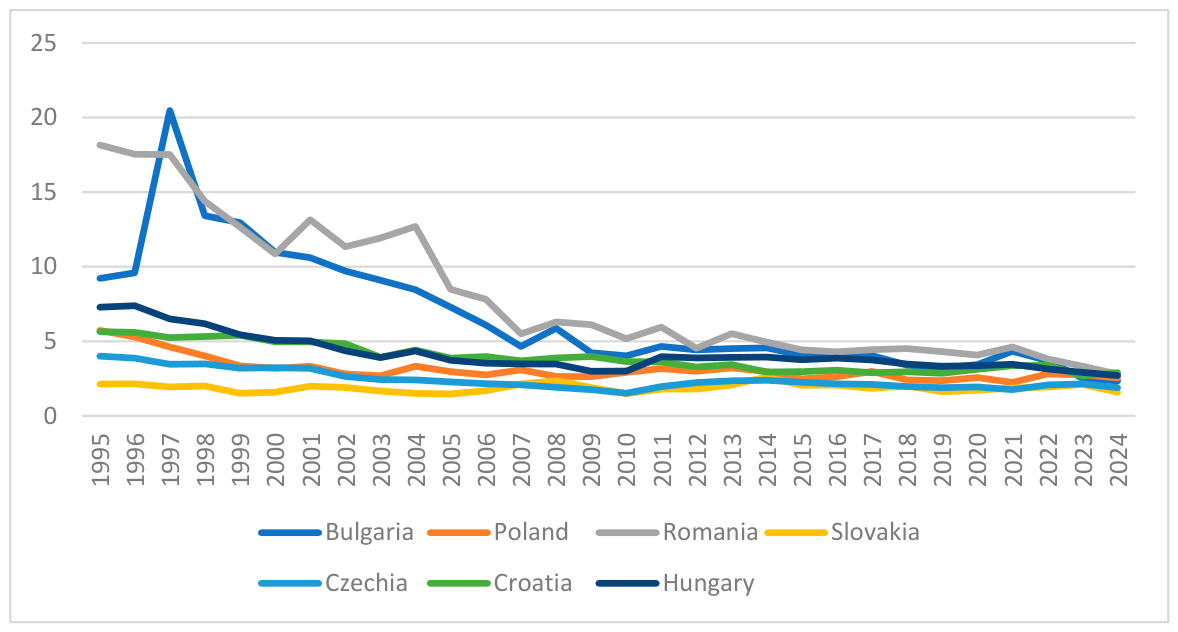
| H1 Over the period 1995–2024, the agricultural share in GDP has followed a significant downward trend across Central and Eastern European countries, starting from significantly different initial structural levels (Downward trend dimension) | Descriptive statistics and time-series trend analysis, β-convergence | All seven countries exhibit a clear declining trajectory; highest values concentrated in the 1990s, followed by sustained decreases, especially in Romania and Bulgaria. | Accepted |
| H1 Over the period 1995–2024, the agricultural share in GDP has followed a significant downward trend across Central and Eastern European countries, starting from significantly different initial structural levels (Structural heterogenity dimension) | Comparative descriptive analysis (mean, min–max, coefficient of variation), β-convergence | Romania (≈8.04%) and Bulgaria (≈6.66%) start from much higher levels than Czechia and Slovakia; very high coefficients of variation (>50%) confirm heterogeneity. | Accepted |
| H2 The agricultural share in GDP exhibits a long-term convergence process across the analyzed economies, accompanied by a strong cross-country synchronization of dynamics that reflects the influence of common regional factors. (Convergence dimension) | Dispersion analysis, Spearman correlations, Ward cluster analysis, σ-convergence | Post-2015 values cluster within ~1.5–3.5% of GDP; strong positive correlations and clear grouping patterns indicate structural convergence. | Accepted |
| H2 The agricultural share in GDP exhibits a long-term convergence process across the analyzed economies, accompanied by a strong cross-country synchronization of dynamics that reflects the influence of common regional factors. (Synchronization dimension). | Spearman correlation matrix and hierarchical clustering, σ-convergence, | Strong and very strong correlations among most countries; however, Slovakia shows near-zero correlations and late clustering, indicating atypical behavior. | Partially accepted |
| H3 (methodological precondition) The time series of the agricultural share in GDP deviates from the normality assumption for the majority of the countries considered and are integrated of order one (I(1)), thereby justifying the use of non-parametric dependence measures and differenced (ARIMA) modelling (Non-normality dimension) | Shapiro–Wilk normality test | p-values < 0.01 for six countries lead to rejection of normality; only Slovakia (p = 0.271) is compatible with normal distribution. | Accepted |
| H3 (methodological precondition) The time series of the agricultural share in GDP deviates from the normality assumption for the majority of the countries considered and are integrated of order one (I(1)), thereby justifying the use of non-parametric dependence measures and differenced (ARIMA) modelling. (integration dimension). | Augmented Dickey–Fuller (ADF) unit root tests | Series are non-stationary in level but stationary after first differencing for all countries (p < 0.05 for D(AGRI)). | Accepted |
| H4 Adequately specified ARIMA models capture the dynamics of the agricultural share in GDP and indicate a continued decline or stabilization of this share across the analyzed economies over the medium term (Modelling adequacy dimension) | Information criteria (AIC, SC), residual diagnostics (B–G, ARCH, DW), forecast accuracy (RMSE, MAPE) | Optimal models pass diagnostic tests and display lower forecast errors compared with alternatives. | Accepted |
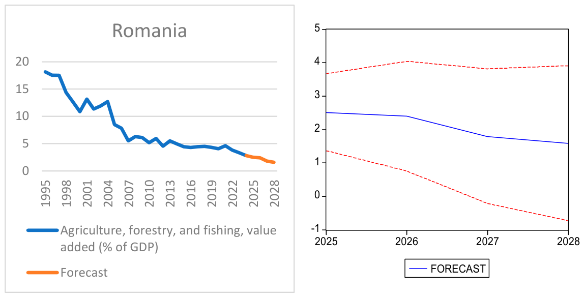
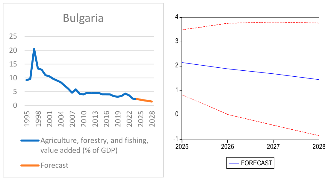
| H4 Adequately specified ARIMA models capture the dynamics of the agricultural share in GDP and indicate a continued decline or stabilization of this share across the analyzed economies over the medium term (Forecasting trajectory dimension). | ARIMA forecasts (2025–2028) | Most countries show gradual decline (Romania, Bulgaria, Czechia) or low-level stabilization (Hungary, Poland, Croatia); Slovakia remains low but more volatile. | Accepted |
Disclaimer/Publisher’s Note: The statements, opinions and data contained in all publications are solely those of the individual author(s) and contributor(s) and not of MDPI and/or the editor(s). MDPI and/or the editor(s) disclaim responsibility for any injury to people or property resulting from any ideas, methods, instructions or products referred to in the content. |
© 2026 by the authors. Licensee MDPI, Basel, Switzerland. This article is an open access article distributed under the terms and conditions of the Creative Commons Attribution (CC BY) license.
Share and Cite
Popescu, L.; Găman, M.; Mihai, L.S.; Drăgan, C.O. Convergence of the Agricultural Share in GDP in Central and Eastern Europe: A Statistical and Econometric Analysis. Economies 2026, 14, 289. https://doi.org/10.3390/economies14070289
Popescu L, Găman M, Mihai LS, Drăgan CO. Convergence of the Agricultural Share in GDP in Central and Eastern Europe: A Statistical and Econometric Analysis. Economies. 2026; 14(7):289. https://doi.org/10.3390/economies14070289
Chicago/Turabian StylePopescu, Liviu, Mirela Găman, Laurențiu Stelian Mihai, and Cristian Ovidiu Drăgan. 2026. "Convergence of the Agricultural Share in GDP in Central and Eastern Europe: A Statistical and Econometric Analysis" Economies 14, no. 7: 289. https://doi.org/10.3390/economies14070289
APA StylePopescu, L., Găman, M., Mihai, L. S., & Drăgan, C. O. (2026). Convergence of the Agricultural Share in GDP in Central and Eastern Europe: A Statistical and Econometric Analysis. Economies, 14(7), 289. https://doi.org/10.3390/economies14070289