From Regime Detection to Decision Rules: A Data-Driven Macro-Financial CVaR Framework for European Multi-Asset Portfolios

Abstract

Weekly macro-financial and financial market data, combined with machine learning methods, offer new possibilities for identifying latent economic states in real time, but the portfolio value of regime detection depends critically on how detected states are translated into allocation rules. This paper develops and evaluates a data-driven macro-financial framework that combines a four-state Gaussian Hidden Markov Model (HMM), estimated on eight weekly macro-financial features, with Conditional Value-at-Risk (CVaR) portfolio optimization across European multi-asset portfolios from January 2000 to April 2026. Using a strictly out-of-sample walk-forward design, we show that naive regime-conditional CVaR allocation generates excessive turnover (approximately 226% per year) that erodes net performance below a simple benchmark under any realistic transaction cost, whereas implementation-aware alternatives recover the gap substantially: regime-constrained weight bands attain a net Sharpe ratio within 0.009 of the static benchmark at roughly 29% annual turnover. Expanding the universe to include sovereign bonds improves drawdown control but introduces duration risk that materializes in rate-hiking episodes. These findings demonstrate that, in data-driven macro-financial systems, the bottleneck is not regime detection but transparent, stable, and cost-aware decision-rule design, with implications for next-generation, AI-assisted macro-financial monitoring and policy surveillance systems.

1. Introduction

The increasing availability of weekly macro-financial and financial market data and the development of machine learning methods for economic analysis have opened new possibilities for identifying latent economic states in real time (Gu et al., 2020). From traditional Hamilton (1989) and Rabiner (1989) Hidden Markov Models for business-cycle identification to data-rich macroeconomic nowcasting frameworks (Bernanke & Boivin, 2003), the common premise is that financial and economic processes cycle through distinct regimes with different statistical properties. In the context of portfolio risk management, such regime information is potentially valuable: an allocation framework that can adapt to changing macroeconomic conditions, such as volatile-stress episodes, sovereign spread crises, or inflation surges, may achieve better risk-adjusted outcomes than a static, regime-unconditional approach.

Yet the empirical evidence on whether regime-conditional portfolio strategies deliver out-of-sample improvements remains mixed, and implementation frictions have received comparatively little systematic attention in the data-driven macroeconomics literature (see Ul-Durar et al., 2025, for a recent review of tail-dependent and distributional approaches in economic analysis). This question is central to the next generation of data-driven and AI-based macroeconomic systems, where the value of a model depends not only on its detection accuracy but also on whether its outputs can be turned into transparent, auditable decisions, an issue of growing relevance for both portfolio risk management and macro-financial policy surveillance.

Regime detection is directly relevant to macro-financial surveillance and systemic risk monitoring (Billio et al., 2012; Adrian & Brunnermeier, 2016). The states identified by Hidden Markov Models (HMMs) estimated on macro-financial features such as implied volatility indices, sovereign credit spreads, yield-curve slope, and inflation measures correspond to recognizable economic episodes: low-volatility expansion phases, broad risk-on regimes, neutral moderate states, and elevated-risk stress periods characterized by financial market distress and widening peripheral spreads. Such classifications provide a transparent, data-driven taxonomy of macro-financial conditions that complements traditional business-cycle dating and can be computed in near-real time. From a systemic risk perspective, the ability to characterize stress regimes and quantify the uncertainty in those labels is a prerequisite for adaptive risk management in next-generation macro-financial systems.

However, regime detection is not equivalent to regime-based decision-making. The central question is not only whether regimes can be detected, but whether detected regimes can be translated into transparent, stable, and low-turnover decision rules. In portfolio optimization, regime transitions can trigger discontinuous changes in the optimization problem, generating excessive rebalancing that erodes any gross performance advantage through transaction costs. This implementation friction is a structural feature of regime-conditional allocation, not an incidental artifact: it arises because the optimal solution for one regime’s scenario set may differ substantially from the optimal solution for an adjacent regime’s set and because the HMM assigns new labels at every rebalance step. Understanding exactly when and why this friction dominates detection quality, and how implementation-aware design can overcome it, is the central methodological contribution of this paper.

The European multi-asset setting provides a particularly demanding test environment. Europe has experienced four structurally distinct macro episodes within the 26-year data sample studied here (January 2000 to April 2026; out-of-sample evaluation begins in 2003 for Panel A and 2010 for Panel B, after the regime-model burn-in): the post-dot-com normalization of 2002 to 2006; the Global Financial Crisis of 2008 to 2009, during which European equity indices lost approximately 50% to 60%; the European sovereign debt crisis of 2011 to 2012, characterized by peripheral spread widening and ECB unconventional policy interventions; and the COVID-19 crash of March 2020, followed by the post-zero-interest-rate transition of 2022, in which the ECB raised its deposit rate by approximately 250 basis points over the course of 2022 (from −0.50% to 2.00%), imposing severe losses on long-duration bonds. Each episode rewarded a different defensive allocation: commodities and gold in 2008, government bonds in 2011, and commodity positions again in 2022. This structural instability in the cross-asset correlation regime (Longin & Solnik, 2001), combined with the presence of rate-shock and sovereign spread dynamics absent in typical US-centric analyses, makes Europe an informative and challenging test bed for evaluating data-driven macro-financial allocation frameworks.

This paper develops and evaluates a transparent data-driven regime framework combining Conditional Value-at-Risk (CVaR) portfolio optimization with a four-state Gaussian HMM estimated on eight weekly macro-financial features, applied to ten risky European assets over January 2000 to April 2026. The HMM generates strictly out-of-sample regime labels via an expanding walk-forward procedure that re-estimates the model at each four-week rebalance step, ensuring no forward-looking information enters portfolio construction. We evaluate naive regime-conditional CVaR (restricting the scenario set to regime-matched historical returns), implementation-aware alternatives (turnover-penalized LP and regime-constrained weight bands), and a 14-asset fixed-income expansion adding sovereign bond indices from Germany, Spain, and Italy.

The results indicate that the main bottleneck is not the identification of regimes but their translation into stable, low-cost allocation rules. The walk-forward HMM produces locally stable, economically interpretable labels, yet naive regime-conditional scenario filtering generates implementation frictions that erode out-of-sample performance. Implementation-aware designs reduce this friction substantially. The fixed-income expansion shows that the defensive channel depends strongly on the asset universe and the prevailing interest-rate environment.

This paper makes three distinct contributions to the literature on next-generation data-driven macroeconomic systems. First, it provides the first strictly out-of-sample evaluation of regime-conditional CVaR specifically designed to isolate the role of implementation friction, extending Guidolin and Timmermann (2007) and Ang and Bekaert (2002, 2004) to the question of decision-rule design, an aspect almost entirely absent from prior empirical regime-portfolio work. Second, it identifies the LP scenario discontinuity as the structural mechanism behind regime CVaR failure: this diagnostic insight directly informs the design of AI-assisted macro-financial monitoring systems, where accurate state detection alone is not sufficient, and the decision layer must be explicitly engineered for cost efficiency and stability. Third, it introduces regime-constrained weight bands as an institutionally viable bridge between macro-state detection and portfolio implementation, achieving near-benchmark risk-adjusted performance at a fraction of the turnover cost. Together, these contributions provide a practical blueprint for the next generation of data-driven allocation frameworks operating under real-world transaction costs and macro-financial regime uncertainty. Relative to the wider literature on tail-sensitive and distributional methods for economic analysis (Ul-Durar et al., 2025), this study is, to our knowledge, the first to embed CVaR tail-risk optimization within a strictly out-of-sample macro-financial regime framework and to identify the LP decision layer—rather than regime detection—as the binding constraint on practical performance.

Recent machine learning approaches to portfolio management, including deep reinforcement learning (Jiang et al., 2017), long short-term memory networks (Fischer & Krauss, 2018), and attention-based sequence models, have demonstrated strong in-sample pattern recognition but typically operate as black-box systems without explicit structural representation of the underlying economic state. Our framework deliberately prioritizes interpretability, auditability, and explicit macro-financial regime labeling over unconstrained predictive capacity, properties that are increasingly required for the responsible deployment of AI-assisted systems in regulated investment management and macro-financial policy surveillance (Gu et al., 2020). The four HMM states can be examined, challenged, and overridden by a risk committee; the decision rules are fully transparent; and the failure mode (excessive turnover under naive regime conditioning) is mechanistically diagnosable, not an opaque output of a gradient-descent optimizer.

The remainder of this paper is organized as follows. Section 2 describes the data, features, model specifications, and backtesting design. Section 3 reports the empirical results across six subsections covering regime characterization, baseline performance, turnover analysis, implementation-aware variants, fixed-income expansion, and robustness checks. Section 4 discusses the findings in relation to data-driven macroeconomics, AI/machine learning systems, systemic risk, and implementation cost transparency. Section 5 concludes.

2. Materials and Methods

2.1. Data and Asset Universe

The baseline investable universe consists of ten risky assets and one risk-free rate, all denominated in or converted to euros. The risky universe spans European equities (six indices: CAC 40, DAX, EuroStoxx 50, FTSE MIB, IBEX 35, and STOXX Europe 600), listed real estate (FTSE EPRA/NAREIT Europe), broad commodities (Bloomberg Commodity Index), energy (Brent crude oil front-month futures), and precious metals (gold spot, EUR-converted from USD). The risk-free instrument is the EURIBOR 3-month rate, used as the cash return benchmark and excluded from risky portfolio optimization. All series are sourced from LSEG Workspace (Refinitiv) as weekly Friday-close prices. Exceptions: Brent is a front-month futures price (RIC: LCOc1); gold is a USD spot price (XAU=) converted at weekly prevailing FX rates; and EURIBOR 3M (EUR3MD=) is a rate series converted to a weekly simple return. A 14-asset FI-expanded universe for robustness adds Germany, Spain, and Italy government bond total-return indices from FTSE Russell.

Table 1. Asset universe.

Asset	Type	RIC	Notes
EURIBOR 3M	Risk-free proxy	EUR3MD=	Rate; weekly simple return; excluded from optimization
Bloomberg Commodity	Commodity (broad)	BCOM	Total-return index
Brent Crude Oil	Energy	LCOc1	Front-month futures price
Gold	Precious metals	XAU=	USD spot; EUR-converted at weekly FX
CAC 40	Equity (FR)	.FCHI	Total return
DAX	Equity (DE)	.GDAXI	Total return
EuroStoxx 50	Equity (Eurozone)	.STOXX50E	Total return
FTSE MIB	Equity (IT)	.FTMIB	Total return
IBEX 35	Equity (ES)	.IBEX	Total return
STOXX Europe 600	Equity (broad EU)	.STOXX	Total return; single-asset benchmark
FTSE EPRA/NAREIT	Listed real estate	.FTEPRAEUR	Total return

The table reports the 11-asset baseline investable universe. RICs are LSEG Workspace identifiers. All return series are in EUR. TR = total-return index. Brent crude oil and gold are price series, not total-return indices. EURIBOR 3M is excluded from the optimized risky portfolio. A 14-asset FI-expanded universe adds Germany, Spain, and Italy government bond TR indices from FTSE Russell; the Italy series (.FTIT_TSYUSDT) is EUR-converted by LSEG.

summarizes the complete universe.

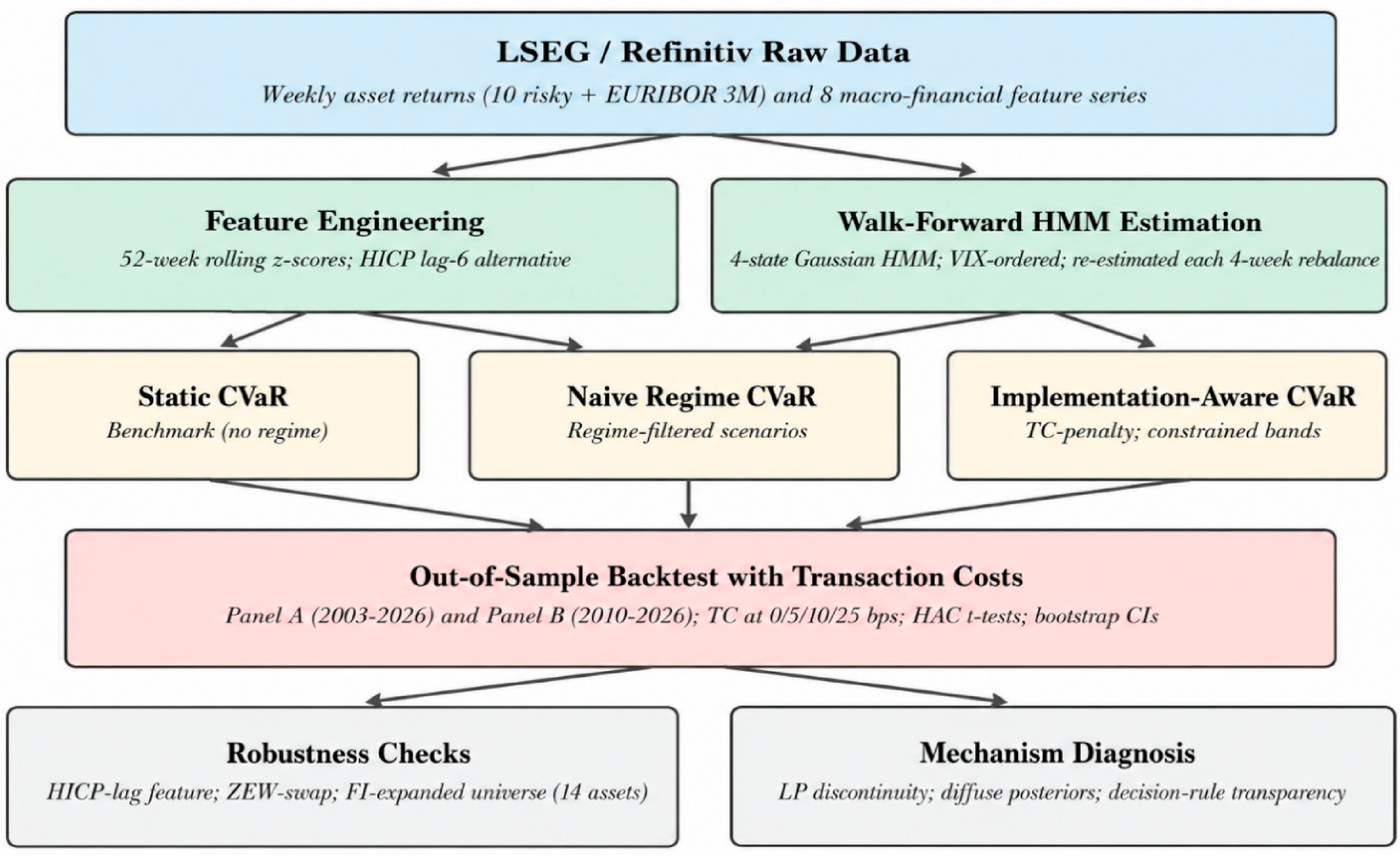
All series are aligned to weekly Friday-close observations over 14 January 2000 to 3 April 2026, yielding 1369 weekly observations before burn-in exclusions. We use simple (arithmetic) weekly returns throughout; all strategy statistics are annualized using a factor of 52. Missing values from national holidays are forward-filled for up to five consecutive business days. Raw source files are subject to LSEG data licensing restrictions and cannot be distributed publicly; all results are reproducible from the processed parquet files accompanying this paper (see Data Availability Statement). Figure 1 summarizes the complete methodological workflow, from raw LSEG/Refinitiv data extraction and return construction to macro-financial regime estimation, portfolio optimization, backtesting, transaction-cost evaluation, and mechanism diagnosis.

2.2. Macro-Financial Regime Features

The HMM is estimated on eight macro-financial features, each transformed to a 52-week rolling z-score to ensure comparable scale. The features are: VIX implied volatility (z52_VIX, primary anchor for state ordering); VSTOXX European implied volatility (z52_VSTOXX); MOVE fixed-income volatility index (z52_MOVE); Germany 10-year yield minus ECB deposit-rate slope (z52_germany_10y_depo_slope); average sovereign spread of Spain, Portugal, and Italy over Germany (z52_peripheral_spread_avg); DXY dollar index (z52_DXY_USD_Index); Eurozone Economic Sentiment Indicator (z52_ESI, monthly, interpolated to weekly); and HICP headline-minus-core inflation gap (z52_hicp_headline_core_gap, approximately 4-week publication lag). Sample coverage ranges from 78% (ESI, HICP) to 100% (VIX). For a given week, the feature vector is constructed using the most recently available observation, with HICP subject to publication-lag risk (see Section 3.6).

This feature set is designed to capture the primary macro-financial dimensions relevant to European multi-asset allocation: volatility and tail-risk sentiment (VIX, VSTOXX, MOVE), fixed-income market stress (sovereign spreads, yield-curve slope), macro growth and inflation pressure (ESI, HICP gap), and global risk appetite (DXY). Together, these features encode the macro-financial information that historically differentiates crisis, recovery, expansion, and stress periods in European markets. Feature selection followed two explicit criteria: First, a minimum 75% weekly coverage over the full 1999–2026 analysis window, ensuring feature availability throughout the walk-forward procedure without excessive imputation. Variables failing this threshold (e.g., raw Germany 10-year government bond yields, which are unavailable after October 2019 in the LSEG series used) were replaced by derived series with full coverage (here, the yield-curve slope constructed using the ECB deposit rate as the short-rate proxy). Second, dimensional coverage: the eight features collectively span five conceptually distinct macro-financial dimensions—volatility and tail-risk sentiment (VIX, VSTOXX, MOVE), fixed-income stress (sovereign spreads, yield-curve slope), macro growth and inflation pressure (ESI, HICP gap), and global risk appetite (DXY)—reducing the risk of a regime classifier dominated by a single factor. A systematic feature-importance analysis lies outside the scope of this paper; the robustness checks in Section 3.6 provide partial empirical evidence that no single feature drives the four-state structure.

2.3. Hidden Markov Model Specification

We model the evolution of market states using a four-state Gaussian Hidden Markov Model (HMM; Hamilton, 1989; Rabiner, 1989; Kim, 1994) with diagonal covariance matrices, estimated via the Expectation–Maximization (EM) algorithm implemented in the hmmlearn library. We use 15 random restarts and up to 500 EM iterations per restart, selecting the solution with the highest log-likelihood. The four-state specification is selected by a Bayesian Information Criterion (BIC) from a grid of two to four states; in all walk-forward windows, four states is consistently preferred. States are ordered post-estimation by ascending mean z52_VIX, so that State 0 has the lowest equity-volatility signature (Low-vol/Subdued) and State 3 the highest (Elevated-risk/Stress).

As an additional robustness check, we subsequently evaluated K = 5 on the full sample. The BIC progression across all candidates is K = 2: 22,912; K = 3: 21,882 (ΔBIC = −1030 vs. K = 2); K = 4: 21,244 (ΔBIC = −638 vs. K = 3); K = 5: 20,769 (ΔBIC = −475 vs. K = 4). The diminishing marginal improvement (−1030 → −638 → −475) indicates a clear elbow at K = 4. The K = 5 solution decomposes the elevated-risk state into two economically distinguishable sub-regimes—a peripheral spread stress state (dominant during the 2010–2012 sovereign debt crisis) and a pure equity-volatility shock state (dominant in 2008 and 2020)—and introduces a strong-USD/inflation transition state capturing the 2022 rate-shock environment. While this decomposition is economically coherent, K = 4 was retained for parsimony: each additional state adds 2K − 1 = 9 transition parameters, and the core finding is invariant to the choice between K = 4 and K = 5. The LP scenario discontinuity driving excess turnover is a structural property of unconstrained regime-conditional CVaR regardless of regime count, and regime-constrained weight bands—our proposed remedy—produce equivalent turnover reductions under either specification.

The K = 4 specification is also consistent across estimation windows: the four macro-financial states retain stable mean-feature signatures and economic interpretations throughout the walk-forward period, confirming that the four-state structure is a persistent feature of the European macro-financial data rather than an artifact of any particular estimation subsample.

All regime labels used in portfolio construction are strictly out-of-sample. We implement an expanding walk-forward procedure: at each four-week rebalance step, the HMM is re-estimated from scratch on all available history up to the rebalance date, subject to a minimum of 156 weeks (three years) of training data. Panel B evaluation begins in October 2010 (full backtesting windows are defined in Section 2.6), which ensures stable four-state estimates. The walk-forward design contrasts with the partial in-sample evaluations common in earlier regime-switching portfolio work (Guidolin & Timmermann, 2007) and ensures that all reported performance metrics reflect genuine predictive content. Posterior state probabilities are soft assignments; the hard-assignment regime label is the argmax state at each week.

2.4. CVaR Portfolio Optimization

For a portfolio weight vector w, the Conditional Value-at-Risk (CVaR) at confidence level α = 0.95 is the expected loss conditional on being in the worst (1 − α) = 5% tail of the return distribution. CVaR is a coherent risk measure (Acerbi & Tasche, 2002) with superior tail sensitivity relative to VaR-based approaches (Engle & Manganelli, 2004). Following Rockafellar and Uryasev (2000) and Krokhmal et al. (2002), CVaR is minimized via a linear program (LP) over a scenario set of $T_s$ = 260 historical weekly returns, as in Equation (1):

$$\underset{w,\zeta ,u}{\mathrm{m}\mathrm{i}\mathrm{n}} \zeta +{\displaystyle \frac{1}{(1-\alpha )·T_s}}·{\displaystyle {\sum }_{t=1}^{T_s}}{u}_t$$

(1)

$$\mathrm{s}.\mathrm{t}. u_t\ge -r_t^{\prime }w-\zeta , u_t\ge 0, {\sum }_i{w}_i=1, 0\le w_i\le 0.25$$

(2)

where ζ is the VaR threshold and $u_t$ are auxiliary loss exceedance variables (Equation (2)). The 25% maximum weight per asset prevents concentration risk. The scenario window is a rolling 260-week (5-year) history.

We solve the LP using scipy.optimize.linprog at each four-week rebalance. As an additional benchmark, a Markowitz (1952) minimum-variance portfolio is estimated with a Ledoit–Wolf shrinkage covariance matrix (Ledoit & Wolf, 2004) and the same 25% weight cap.

2.5. Regime-Conditional and Implementation-Aware Allocation Rules

We evaluate four allocation rules that use the HMM regime signal. Static CVaR uses the full 260-week scenario window without regime conditioning and serves as the primary benchmark. Regime CVaR-A, the naive regime-conditional specification, restricts the scenario set to historical weeks assigned to the current walk-forward regime. If fewer than 30 regime-matched observations are available, the optimizer falls back to the full 260-week window. Weighted CVaR instead retains the full scenario window and weights historical scenarios according to the current HMM posterior probabilities.

Two implementation-aware rules are introduced to address the turnover channel. The first augments the CVaR objective with an L1 penalty on changes relative to the drift-adjusted portfolio from the previous rebalance. The second replaces this penalty with an explicit turnover budget. Both formulations preserve linear-programming tractability through auxiliary variables, as detailed in Appendix A.

A separate regime-constrained CVaR specification keeps the full 260-week scenario window unchanged but allows the HMM state to modify group-level portfolio constraints. In stress states, the equity cap is reduced to 45% and the defensive-asset floor is increased to 30%. In risk-on states, the equity cap is relaxed to 75% and the defensive-asset floor is set at 10%. Defensive assets are defined as gold, the Bloomberg Commodity Index, and Brent crude oil. The complete constraint map across all four states is reported in Appendix A.3. This design translates regime information into transparent investment policy guardrails rather than changing the historical scenario set itself.

2.6. Backtesting Design, Transaction Costs, and Statistical Inference

All strategies are rebalanced every four weeks. Panel A evaluates the long-horizon period from 10 January 2003 to 3 April 2026 (1213 weeks) for non-regime strategies. Panel B evaluates the period from 15 October 2010 to 3 April 2026 (808 weeks) and includes all regime-conditional strategies.

Performance metrics include annualized CAGR, annualized volatility, Sharpe ratio, maximum drawdown, 95% CVaR, Calmar ratio, and annualized turnover. The Sharpe ratio is computed using weekly excess returns over EURIBOR 3M and annualized by multiplying by the square root of 52. CAGR and volatility are annualized from weekly returns using the standard factor of 52.

Turnover is computed at each rebalance as the one-way traded portfolio weight, defined as one half of the sum of absolute changes between the target portfolio and the drift-adjusted portfolio immediately before rebalancing. Annualized turnover is then obtained from the weekly turnover series, with zero turnover assigned to non-rebalance weeks, by multiplying its weekly average by 52. Equivalently, for a four-week rebalance cycle, this corresponds approximately to average turnover per rebalance multiplied by 13. Transaction costs are applied to the lagged turnover series at rates of 0, 5, 10, and 25 basis points. Statistical inference on excess-return differentials relies on heteroskedasticity- and autocorrelation-consistent (HAC) t-statistics computed with Newey–West standard errors (Newey & West, 1987) at a lag of 13 weeks, complemented by circular block-bootstrap confidence intervals for the Sharpe ratios.

3. Results

3.1. Macro-Financial Regime Characterization

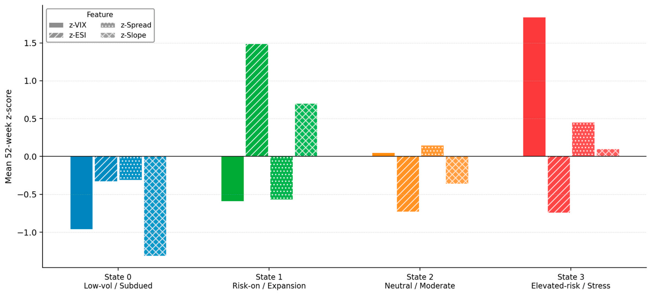
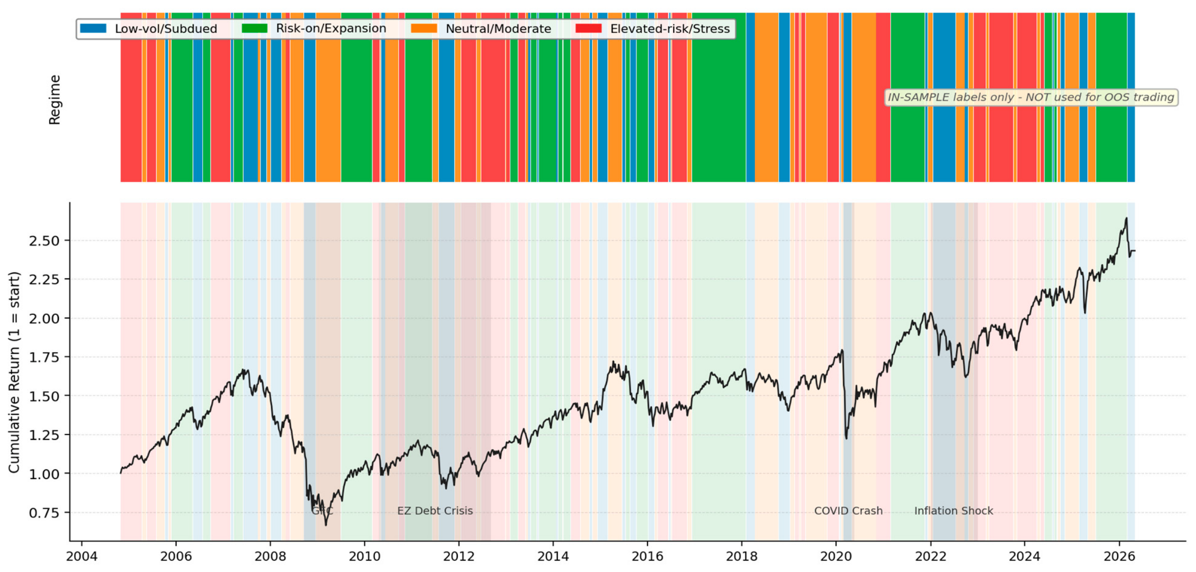
The four HMM states are ordered by ascending mean implied volatility z-scores (z-VIX), yielding an economically intuitive volatility ladder: State 0 (Low-vol/Subdued) to State 3 (Elevated-risk/Stress). Figure 2 displays the mean 52-week z-scores of the four key macro-financial features across states;

Table 2. HMM market-state characteristics.

State	Label	Freq%	Avg Dur (w)	z52 VIX	z52 ESI	z52 Spread	z52 Slope
0	Low-vol/Subdued	24.8	13.3	−0.96	−0.33	−0.31	−1.31
1	Risk-on/Expansion	28.5	18.8	−0.59	+1.49	−0.57	+0.70
2	Neutral/Moderate	26.9	7.9	+0.05	−0.73	+0.15	−0.36
3	Elevated-risk/Stress	19.8	7.2	+1.84	−0.74	+0.45	+0.10

Four-state Gaussian HMM estimated on eight macro-financial z-score features (full-sample descriptive; portfolio construction uses strictly out-of-sample walk-forward labels). States ordered by ascending mean z52_VIX. Freq = share of weekly observations. Avg Dur = average episode duration (weeks). ESI = Economic Sentiment Indicator; Spread = average ES/PT/IT peripheral spread to Germany. HMM: Hidden Markov Model; VIX: CBOE Volatility Index.

provides full descriptive statistics. The state characteristics are consistent with recognizable European macro-financial episodes: State 1 (Risk-on/Expansion) captures broad growth phases, while State 3 identifies the Global Financial Crisis of 2008 to 2009, the European sovereign crisis of 2011 to 2012, and the COVID-19 crash of March 2020. These labels are interpretive, not model constraints; portfolio construction uses exclusively out-of-sample walk-forward labels (Figure 3).

3.2. Static CVaR and Naive Regime Conditioning

Table 3. Panel A Performance: Long-Horizon Evaluation, 2003 to 2026.

Strategy	CAGR%	Vol%	Sharpe	MaxDD%	CVaR95%	Calmar	Ann.TO%
Equal-Weight Risky (1/N)	5.89	15.24	0.368	−50.1	−5.24	0.118	36.3
STOXX Europe 600	4.47	17.50	0.265	−60.2	−5.94	0.074	0.0
Static CVaR	7.05	12.22	0.513	−39.5	−4.19	0.179	24.9
Markowitz (Min-Var)	5.65	12.02	0.409	−45.6	−4.27	0.124	16.8

Weekly simple returns, 1213 observations (10 January 2003 to 3 April 2026). Gross performance at 0 bps transaction costs. Annualization factor 52. CAGR = compound annual growth rate. Vol = annualized standard deviation. Sharpe = (mean excess weekly return/SD excess) × sqrt(52) relative to EURIBOR 3M. MaxDD = maximum drawdown. CVaR 95% = average of worst 5% weekly returns. Ann.TO = annualized one-way portfolio turnover. Bootstrap 95% CI: circular block bootstrap, block = 13 weeks, 5000 draws.

reports Panel A performance (1213 weeks, 2003 to 2026). Static CVaR achieves the highest Sharpe ratio (0.513) and the lowest maximum drawdown (−39.5%) among all non-regime strategies, substantially better than the equal-weight (1/N) benchmark (DeMiguel et al., 2009) (−50.1%) and the STOXX Europe 600 single-asset benchmark (−60.2%). The risk reduction reflects the CVaR LP systematically concentrating in gold and Bloomberg Commodity (approximately 50% combined weight), which function as tail-risk dampeners in the absence of sovereign bonds. No strategy achieves a statistically significant excess-return differential over the equal-weight benchmark (HAC t-statistics below 1).

Table 4. Panel B performance: regime-aware out-of-sample evaluation, 2010 to 2026.

Strategy	CAGR%	Vol%	Sharpe	MaxDD%	CVaR95%	Ann.TO%
Equal-Weight Risky (1/N)	5.65	14.43	0.409	−32.8	−4.81	35.2
STOXX Europe 600	5.28	15.86	0.363	−31.9	−5.33	0.0
Static CVaR	6.03	10.97	0.530	−25.3	−3.60	21.4
Markowitz (Min-Var)	5.03	10.85	0.447	−24.9	−3.64	12.3
Regime CVaR-A	4.35	11.78	0.365	−25.8	−3.96	225.8
Weighted CVaR	4.35	11.62	0.368	−25.4	−3.88	232.5

Weekly simple returns, 808 observations (15 October 2010 to 3 April 2026). Gross performance at 0 bps transaction costs. HMM MIN_TRAIN_OBS = 156 weeks; all regime labels are strictly out-of-sample (walk-forward expanding window). Definitions as in Table 3. CVaR: Conditional Value-at-Risk; HMM: Hidden Markov Model.

presents Panel B results (808 weeks, 2010 to 2026). Static CVaR remains the most robust benchmark with a Sharpe of 0.530. The naive Regime CVaR-A generates a gross Sharpe of only 0.365, and Weighted CVaR 0.368, both below the equal-weight benchmark (0.409). The underperformance is not attributable to poor regime detection but to the implementation friction documented in the next subsection.

3.3. Turnover and the Transaction-Cost Channel

Table 5. Transaction-cost sensitivity, Panel B (net Sharpe ratio).

Strategy	0 bps	5 bps	10 bps	25 bps	Ann.TO%
Equal-Weight Risky (1/N)	0.409	0.407	0.406	0.403	35.2
STOXX Europe 600	0.363	0.363	0.363	0.363	0.0
Static CVaR	0.530	0.529	0.528	0.525	21.4
Markowitz (Min-Var)	0.447	0.446	0.445	0.444	12.3
Regime CVaR-A	0.365	0.355	0.346	0.317	225.8
Weighted CVaR	0.368	0.358	0.348	0.318	232.5

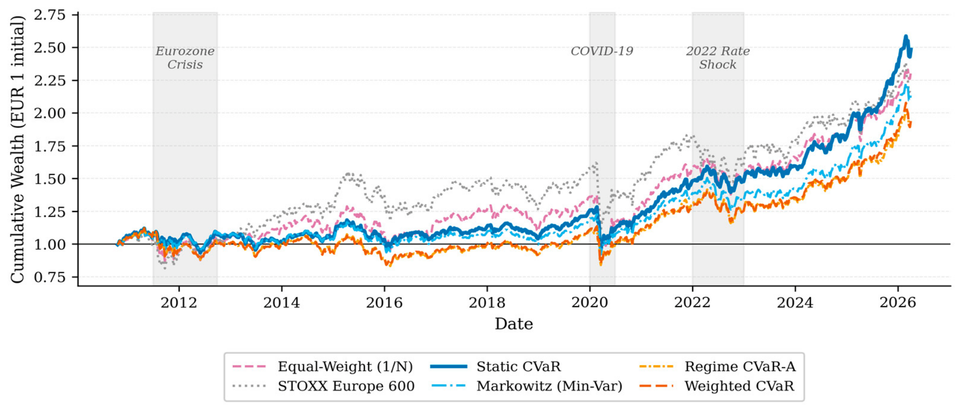
Net Sharpe ratios at four transaction-cost (TC) levels (0, 5, 10, 25 bps per one-way unit of turnover). Annual turnover reported at gross (TC = 0) level. TC is subtracted from gross weekly returns before computing Sharpe. CVaR: Conditional Value-at-Risk.

reports the transaction-cost sensitivity of all strategies. Regime CVaR-A annual turnover is 225.8%, approximately 17.4% per four-week rebalance. Weighted CVaR is similar at 232.5%. By contrast, Static CVaR turns over only 21.4% annually. At 10 basis points of transaction cost, the net Sharpe of Regime CVaR-A falls to 0.346, and Weighted CVaR to 0.348, compared to 0.528 for Static CVaR and 0.406 for equal-weight. At 25 bps, the regime strategies register net Sharpe ratios of 0.317 and 0.318, respectively. The performance degradation is approximately linear in TC_rate times the turnover differential, confirming that turnover, not scenario filtering per se, is the dominant driver of net performance differences, see Figure 4.

The transaction-cost levels considered here (0–25 bps one-way) are consistent with empirical estimates of trading costs for liquid instruments documented in the asset-pricing literature (Frazzini et al., 2015; Novy-Marx & Velikov, 2016).

This tenfold turnover differential arises because each regime transition causes the CVaR LP scenario set to change discontinuously, producing abrupt portfolio reconstitution at every state switch.

Table 6. Statistical tests, Panel B (2010 to 2026).

Strategy	Ann. Diff	t-Stat	p(1-Sided)	Sig	Sharpe	CI Lo	CI Hi
Equal-Weight (1/N)	-	-	-	-	0.409	−0.054	0.926
STOXX Europe 600	−0.13%	−0.096	0.538		0.363	−0.056	0.833
Static CVaR	−0.09%	−0.059	0.523		0.530	+0.068	1.058
Markowitz (Min-Var)	−1.05%	−0.682	0.752		0.447	−0.004	0.962
Regime CVaR-A	−1.60%	−1.227	0.890		0.365	−0.079	0.880
Weighted CVaR	−1.62%	−1.193	0.883		0.368	−0.074	0.891

HAC/Newey–West one-sided t-test on weekly excess-return differentials (strategy minus equal-weight), Newey–West lag = 13 weeks. H_1: strategy mean excess return > benchmark. Panel B: Circular block-bootstrap 95% Sharpe confidence intervals, block = 13 weeks, 5000 draws. Bootstrap CIs report individual strategy Sharpe uncertainty. No test achieves conventional significance. HAC: Heteroskedasticity and autocorrelation consistent.

confirms that no pairwise HAC/Newey–West test achieves conventional significance: bootstrap Sharpe confidence intervals span approximately +−0.4 units for all strategies, so that point estimate differences of 0.1 to 0.2 cannot be conclusively attributed to skill versus sampling variation over the 808-week evaluation window.

3.4. Implementation-Aware Regime Translation

Table 7. TC-aware CVaR and regime-constrained CVaR: selected results2.

Strategy	Gross Sharpe	Net @10bps	Ann.TO%
Panel A: TC-Aware CVaR
Static CVaR, experiment-grid benchmark	0.553	0.551	20.6%
Regime CVaR-A, unconstrained	0.365	0.346	225.8%
Regime CVaR-A, τ = 0.10	0.491	0.486	59.9%
Regime CVaR-A, τ = 0.20	0.449	0.440	101.2%
Weighted CVaR, τ = 0.10	0.492	0.486	61.5%
Weighted CVaR, ZEW + λ = 0.005	0.572	0.567	64.8%
Panel B: Regime-Constrained CVaR (Weight-Band Approach)
Static CVaR, experiment-grid benchmark	0.553	0.551	20.6%
Regime-Constrained CVaR (baseline HMM)	0.522	0.519	29.2%
Regime-Constrained CVaR (ZEW-swap HMM)	0.519	0.517	27.0%
Regime CVaR-A (baseline, for reference)	0.365	0.346	225.8%

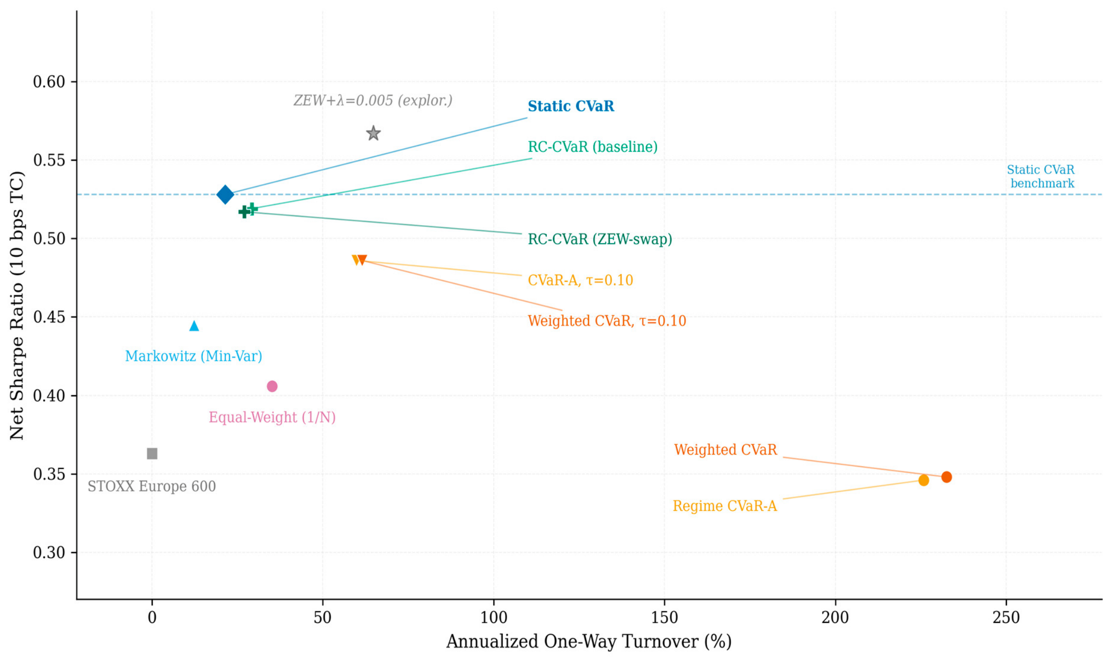
Panel A: TC-aware CVaR with turnover budget (τ) and L1 penalty (λ). Panel B: Regime-constrained CVaR with group-level weight bands varying by HMM state. Evaluation window: 2010 to 2026, 808 weeks. ZEW-swap replaces z52_VSTOXX with z52_ZEW_Germany. Ann.TO = annualized one-way turnover.

1 reports results for the two implementation-aware strategies. Panel A presents TC-aware CVaR specifications. The turnover-constrained specification at τ = 0.10 reduces Regime CVaR-A annual turnover from 225.8% to 59.9%, a reduction of 166 percentage points. Net Sharpe at 10 bps improves from 0.346 to 0.486. Despite these improvements, no TC-aware variant consistently surpasses Static CVaR (net Sharpe 0.551 at 10 bps in this experiment context; see Table 7 note for the scope difference relative to Table 4). The ZEW-swap penalized variant (ZEW + λ = 0.005) produces an exploratory net Sharpe of 0.567, which should not be interpreted as evidence of general outperformance: label agreement with the canonical HMM is only 47.9%, and this result is not confirmed in any other specification.

Panel B of Table 7 presents regime-constrained CVaR results. This approach achieves near-static performance at 0.522 gross Sharpe (baseline HMM) and 0.519 (ZEW-swap HMM), with annual turnover of 29.2% and 27.0%, respectively, a substantial improvement over the 226% turnover of Regime CVaR-A. Net Sharpe at 10 bps reaches 0.519 and 0.517, within 0.009 of Static CVaR. This approach is also more transparent to a risk committee: it encodes a clear investment policy (reduce equity in stress, maintain defensive floor) rather than a less visible adjustment to the LP scenario set. Figure 5 illustrates the turnover versus net Sharpe frontier across all evaluated specifications.

3.5. Sovereign Fixed-Income Expansion

Table 8. FI-expanded universe: performance comparison.

Strategy	Sharpe Base	Sharpe FI-Exp	Delta Sharpe	MaxDD Base	MaxDD FI-Exp	Delta MaxDD
Panel A: 2003 to 2026
Equal-Weight Risky	0.368	0.313	−0.055	−50.1%	−38.9%	+11.2 pp
Static CVaR	0.513	0.547	+0.034	−39.5%	−14.8%	+24.7 pp
Markowitz (Min-Var)	0.409	0.447	+0.038	−45.6%	−14.2%	+31.4 pp
Panel B: 2010 to 2026
Static CVaR	0.530	0.504	−0.026	−25.3%	−14.6%	+10.7 pp
Markowitz (Min-Var)	0.447	0.463	+0.016	−24.9%	−14.4%	+10.5 pp
Regime CVaR-A	0.365	0.430	+0.065	−25.8%	−17.2%	+8.6 pp
Weighted CVaR	0.368	0.378	+0.010	−25.4%	−16.3%	+9.1 pp

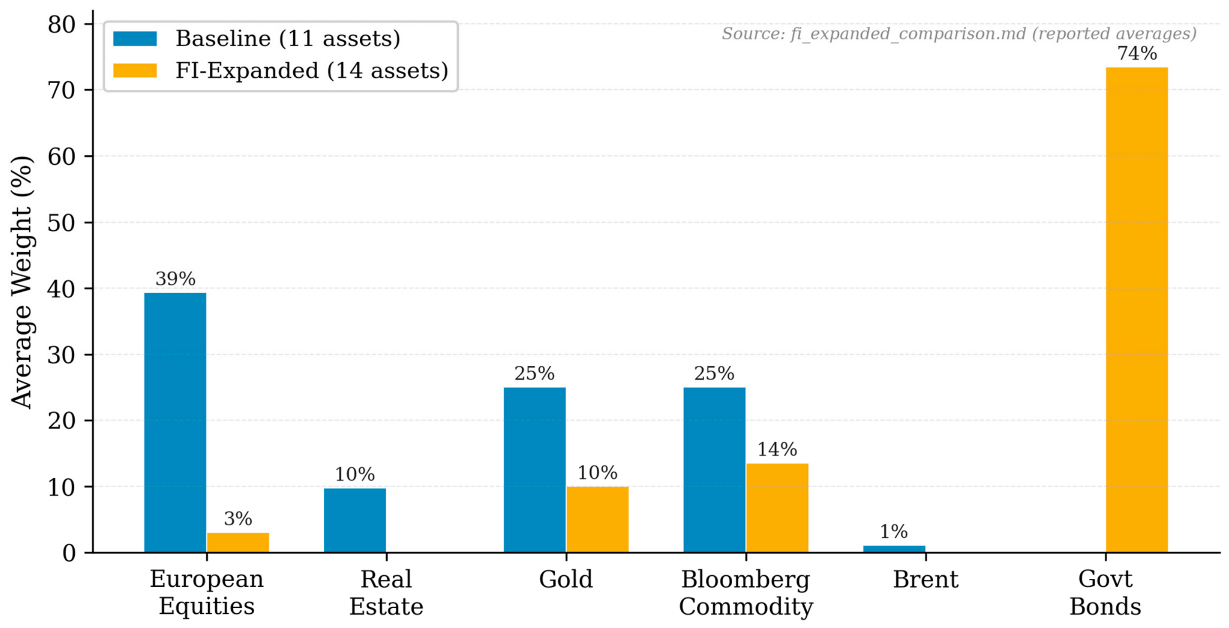
Baseline = 11-asset universe. FI-expanded = 14-asset universe adding Germany, Spain, and Italy government bond TR indices. Gross performance at 0 bps TC. Panel A: 2003 to 2026. Panel B: 2010 to 2026. Delta = FI-expanded minus baseline. The 2022 ECB rate-hiking episode was adverse for FI-expanded portfolios. FI: fixed income; TR: total return; TC: transaction cost.

summarizes FI-expanded results. Panel A (2003 to 2026): adding three government bond total-return indices raises Static CVaR Sharpe from 0.513 to 0.547 (+0.034) while reducing maximum drawdown from −39.5% to −14.8% and annualized volatility from 12.2% to 5.0% (volatility figures computed from the same weekly return series as in Table 3; not tabulated). The bond addition triggers a substantial allocation substitution: the CVaR LP reallocates approximately 73% of the portfolio to sovereign bonds, reducing equity to 3% and gold and commodities combined to 23.5%. This reflects the lower weekly CVaR of government bonds relative to equities and commodities, not a general recommendation to overweight bonds regardless of the rate environment.

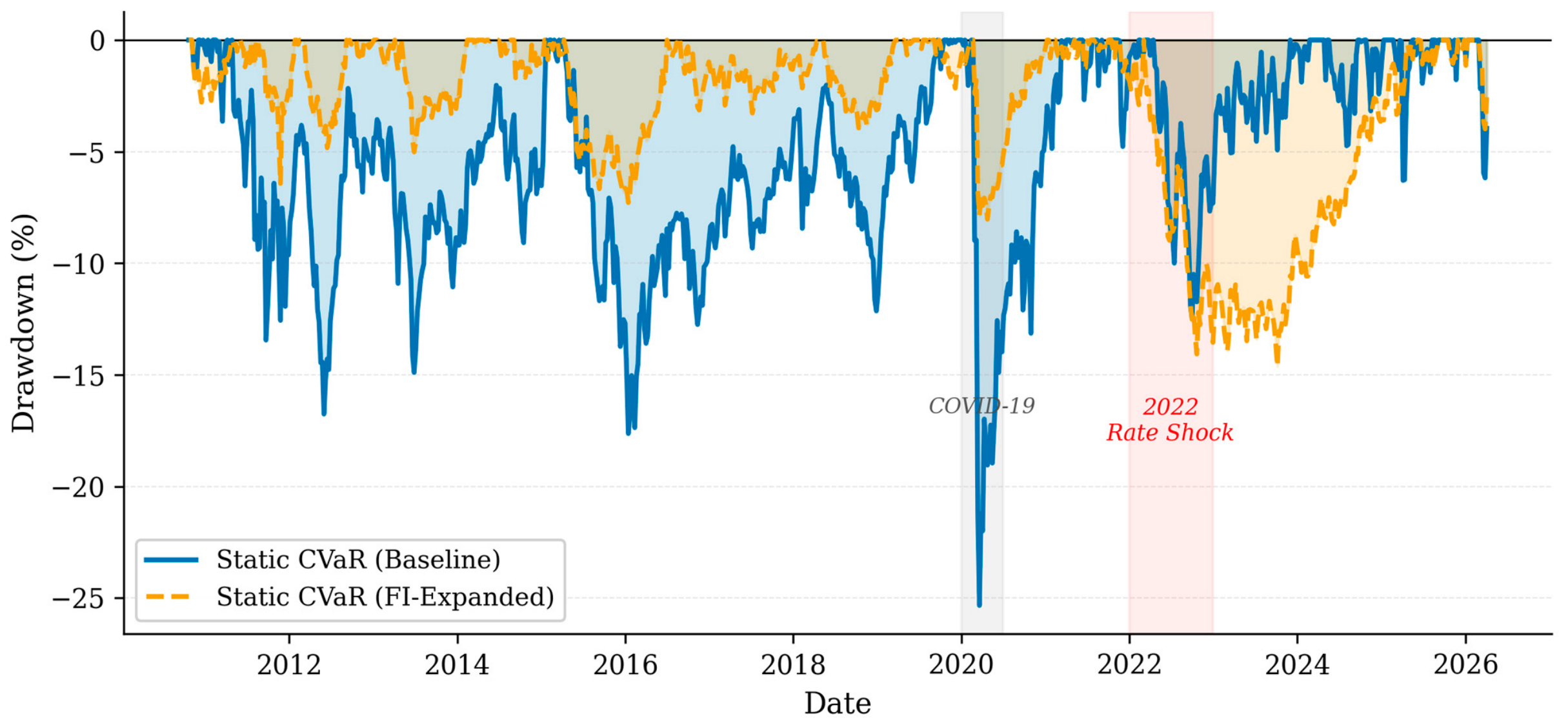
Panel B (2010 to 2026): Static CVaR Sharpe declines slightly (−0.026) despite a material maximum drawdown improvement (−25.3% to −14.6%). The Sharpe decline is explained by the 2022 ECB rate-hiking cycle: with the FI-expanded portfolio holding approximately 75% in sovereign bonds entering 2022, the portfolio recorded losses of approximately −10% while the baseline portfolio held commodities and gold, which rose on energy inflation, see Figure 6 and Figure 7. This illustrates a key practical point: opportunity-set design implicitly takes positions on macro risk factors, and the choice of whether to include fixed income constitutes an implicit bet on rate stability.

3.6. Robustness Checks

We conduct five robustness checks, summarized in

Table 9. Robustness check summary.

Check	Key Finding	Magnitude	Conclusion
HICP lag 6 weeks	Label agreement ~55%; Regime CVaR-A Sharpe changes up to +0.068	Within bootstrap noise	Unchanged
ZEW feature swap	Regime CVaR-A Sharpe: 0.365 to 0.483 (+0.118); label agreement 47.9%; exploratory	No test significance	Unchanged
Rebalance frequency	Lower frequency reduces turnover; 4-week baseline reasonable	No cadence overturns Static CVaR	Unchanged
Turnover smoothing (EWA)	EWA blending reduces turnover ~30%; improves net Sharpe vs. naive regime	Does not surpass Static CVaR	Unchanged
FI-expanded universe	Panel A Sharpe +0.034; Panel B −0.026; MaxDD improved in both panels; 2022 rate-shock adverse	−10% to −13% portfolio loss in 2022	Unchanged

All checks use the Panel B evaluation window (2010 to 2026, 808 weeks). Key metric is net Sharpe at 10 bps for Regime CVaR-A. Delta Sharpe = change vs. baseline. HICP: Harmonized Index of Consumer Prices; ZEW: Zentrum fuer Europaeische Wirtschaftsforschung (In German); EWA: exponential weight averaging; CVaR: Conditional Value-at-Risk.

. First, a 6-week HICP publication-lag correction addresses the risk that HICP data timestamps in LSEG reflect the reference period rather than the release date (approximately 17 days after month-end). Label agreement between baseline and lagged specifications is approximately 55%, confirming that HICP timing is a meaningful but not outcome-determining assumption. The Regime CVaR-A Sharpe changes by up to +0.068, within the bootstrap confidence band.

Second, a ZEW feature swap replaces z52_VSTOXX with z52_ZEW_Germany (unconditional correlation with z52_ESI: r approximately 0.02). This improves Regime CVaR-A point estimates (Sharpe 0.365 to 0.483), but label agreement with the baseline is only 47.9%, and no test achieves statistical significance. These results are exploratory. Third, rebalance frequencies of 1, 2, 4, 8, and 13 weeks are tested; no frequency overturns Static CVaR as the most robust benchmark. Fourth, exponential weight averaging (EWA) blending reduces turnover approximately 30% and improves the net Sharpe versus naive regime baseline but does not surpass Static CVaR. Fifth, the FI-expanded universe robustness is reported in Section 3.5. Across all five checks, the main conclusion is unchanged.

3.7. Mechanism Summary

Table 10. Why Regime CVaR-A fails: mechanism summary.

Mechanism	Root Cause	Empirical Signature	Implementation Fix	Remaining Gap
LP scenario discontinuity	Regime switch replaces entire 260-scenario set with 30–80 matched scenarios	226% annual turnover; tenfold vs. static benchmark	L1 turnover penalty in LP objective reduces TO to 60%	Net SR 0.486 vs. 0.528 for Static CVaR
Small scenario set	CVaR tail estimated from handful of regime-matched observations	Higher OOS estimation error; lower gross Sharpe (0.365 vs. 0.530)	Regime constraints retain full 260-scenario set	Net SR 0.519 vs. 0.528; not statistically significant
Hard label assignment	Argmax discards posterior uncertainty (e.g., 40%/35%/25% spread)	Weighted CVaR soft-weights scenarios but still underperforms static	Soft weighting (Weighted CVaR) partially addresses uncertainty	No improvement over static in any specification
Label sensitivity	HICP-lag6: 55% label agreement; ZEW swap: 47.9% label agreement with baseline	Robustness Sharpe spread <0.02; conclusions unchanged	Feature robustness checks (ZEW swap, HICP lag)	No dominant feature set identified
Macro-portfolio mismatch	Regime signal estimated on macro features; traded assets are financial returns	No asset-level signal decomposition possible with current design	Factor-orthogonal HMM design (not pursued in this paper)	Open research question
Rate-shock exposure (FI)	Bond inclusion changes risk factor profile toward duration	−10% to −13% FI-expanded portfolio losses in 2022 ECB cycle	Explicit duration constraint on bond allocation	Not pursued; opportunity-set design trade-off

Six mechanisms linking regime detection to portfolio implementation failure. Empirical signatures refer to Panel B evaluation window (2010 to 2026, 808 weeks). Net SR = net Sharpe at 10 bps. CVaR: Conditional Value-at-Risk; LP: linear program; HMM: Hidden Markov Model; HICP: Harmonized Index of Consumer Prices; ECB: European Central Bank.

synthesizes the six mechanisms through which naive regime conditional CVaR underperforms the static benchmark, together with the implementation fix pursued in this paper and the remaining performance gap. The table serves as a diagnostic map connecting the theoretical mechanism (LP scenario discontinuity, estimation noise, hard label assignment, label sensitivity, macro-portfolio signal mismatch, and rate-shock exposure) to the empirical evidence and the practical resolution. The formulations underlying each implementation fix are detailed in Appendix A (turnover-penalized and turnover-budgeted LPs) and Appendix A.3 (regime-constrained weight bands).

4. Discussion

4.1. Implications for Next-Generation Macro-Financial Systems

The central result of this paper, that the binding constraint is decision-rule design rather than regime detection, is directly relevant to the theme of ‘Next-Generation Macroeconomics: Data-Driven and Artificial Intelligence Approaches’. The bottleneck is not forecasting or state detection but the design of transparent, auditable, and implementable decision rules. This speaks directly to the transparency and governance of data-driven and AI-based macroeconomic systems: a decision layer that can be audited by a risk committee or a policy authority is a precondition for the responsible deployment of such systems (Gu et al., 2020; Campbell & Viceira, 2002). The European context studied here, spanning the GFC, the sovereign debt crisis, the COVID shock, and the 2022 rate-hiking cycle, provides a stringent real-world test of this principle: detection works, but naive implementation does not.

The HMM states identified here map onto recognizable European macro-financial episodes and are consistent across walk-forward windows, offering interpretability that black-box detectors cannot provide. For systemic risk monitoring, the stress state (State 3) identifies periods of elevated sovereign spread widening, VIX spikes, and deteriorating sentiment, subject to the caveat that state assignments are sensitive to feature construction choices. Three structural mechanisms explain the failure of naive regime conditioning to improve performance. First, restricting to 30 to 80 regime-matched scenarios replaces a well-conditioned optimization with a fragile problem based on a small, historically idiosyncratic sample; estimation error propagates directly to higher turnover. Second, regime transitions cause the entire CVaR scenario set to change discontinuously at each rebalance, generating portfolio reconstitution that is not compensated by return improvements. Third, HMM posteriors are often diffuse in moderate conditions: the hard argmax assignment discards this uncertainty, and even soft-weighted CVaR fails to recover performance, indicating that signal content, not assignment rule, is the binding constraint.

4.2. Implications for Practice and Sovereign Risk Management

The regime-constraints approach is the most practically viable regime-aware mechanism identified in this study. By encoding investment policy beliefs as group-level weight guardrails while keeping the full CVaR scenario set intact, it achieves near-static performance at moderate turnover and produces a policy that can be audited by a risk committee. This approach aligns with how institutional investors use macro views in practice: as overlays on allocation rather than wholesale replacements of the optimization framework, in the spirit of view-based allocation models (Black & Litterman, 1992). The regime-constrained design also generates more stable portfolio sequences over time, reducing operational complexity and capacity constraints that would otherwise further reduce the gross performance advantage of regime-conditional strategies at scale.

The FI-expanded results highlight a second practical implication related to sovereign risk and interest-rate sensitivity. When sovereign bonds are unavailable, the CVaR optimizer concentrates in commodities and gold, which provided effective hedges in the 2022 inflationary episode but performed poorly in the 2008 initial phase of the GFC. Adding bonds produces a more conventional allocation but introduces duration risk that materializes in rate-hiking cycles. Practitioners should be explicit about which macro risk factors their opportunity-set design is implicitly accepting, particularly in a European context where ECB policy and peripheral sovereign spread dynamics create risk exposures absent in typical US-centric frameworks.

A related implication concerns the choice of evaluation benchmark. Static CVaR is a disciplined, systematic strategy with strong risk-control properties; it represents a genuinely demanding bar. Practitioners comparing regime-conditional CVaR to a 60/40 portfolio or an equal-weight benchmark may reach more favorable conclusions, but such comparisons conflate the value of the CVaR optimization framework with the incremental value of regime conditioning, making performance attribution ambiguous.

4.3. Limitations

HMM regime labels are statistical constructs, not causal economic states. The model identifies recurring distributional patterns in the feature vector that need not correspond to structurally distinct regimes in any fundamental sense. The 55% label agreement between baseline and HICP-lagged specifications, and the 47.9% agreement with the ZEW feature swap, suggest that regime assignments are sensitive to feature construction choices in ways that likely reflect measurement uncertainty rather than genuine economic state differences. All downstream portfolio conclusions inherit this uncertainty.

Feature sensitivity is a material concern. The ZEW-swap specification has only 47.9% label agreement with the baseline HMM, indicating that swapping a single feature substantially reorganizes the regime classification. Regime assignments are sensitive to feature construction choices in ways that likely reflect measurement uncertainty rather than genuine economic state differences. Macro release timing introduces potential look-ahead risk for HICP (approximately 4-week publication lag) and ESI (approximately 3-week lag); the HICP-lag6 robustness check addresses HICP specifically, but ESI publication lag is not separately corrected. Practitioners implementing this design should apply publication-lag buffers to all macro features.

The generalizability of these findings beyond European markets deserves discussion. The core mechanism—that LP scenario discontinuity drives excess turnover in naive regime-conditional CVaR, and that regime-constrained weight bands resolve this—is not geographically specific: it is a structural property of the optimization architecture applicable in any multi-asset setting with discrete regime transitions. However, the specific four-state regime structure reflects European institutional features: peripheral sovereign spreads, ECB policy dynamics, and Eurozone-specific growth-inflation cycles. These features have no direct analog in US-centric portfolios, where credit risk is driven by corporate spreads and Federal Reserve policy, or in emerging market contexts, where currency risk and political regimes play a larger role. Applying the framework to other geographies would therefore require recalibrating the macro-financial feature set to the relevant stress channels, and the optimal K may differ. Cross-market validation of the regime-constrained weight-band approach is a natural direction for future research.

The transaction-cost model is simplified: 10 bps one-way covers a range of institutional scenarios but does not model bid–ask spreads on futures contracts, market impact for large trades, or the operational costs of frequent rebalancing. The asset universe excludes corporate credit and inflation-linked bonds, which would add additional dimensions to the diversification and TC modeling. Raw LSEG source data are proprietary. Results are out-of-sample within the 2000 to 2026 European sample but remain sample-specific; generalization to other geographic markets or time periods requires further validation.

The complete Python codebase, including the walk-forward HMM pipeline, CVaR optimization routines, figure-generation scripts, and reproducibility documentation, is publicly available at https://github.com/jorge-grube/PAPER, accessed on 3 June 2026. Raw market data are proprietary (LSEG/Refinitiv) and cannot be redistributed, but the code framework can be applied to any equivalent dataset.

Statistical power is a binding constraint. With 808 weekly observations and a Newey–West HAC lag of 13 weeks, effective degrees of freedom are substantially below nominal. Bootstrap confidence intervals for Sharpe ratios span approximately +−0.4 units, meaning that point estimate differences of 0.1 to 0.2 cannot be conclusively attributed to regime-conditioning skill versus sampling variation. The failure to detect statistically significant outperformance is consistent with both “regime conditioning adds no value” and “the sample is too short to detect realistic Sharpe differences at conventional power.” A longer or geographically diversified replication would sharpen these inferences. The sensitivity of Sharpe ratio inference to estimation error and non-normal returns is itself well documented (Lo, 2002), reinforcing the caution warranted in interpreting these differences.

5. Conclusions

This paper shows that, in data-driven macro-financial systems, the binding constraint is not regime detection but decision-rule design. A four-state Gaussian HMM estimated on eight weekly macro-financial features produces economically interpretable, auditable states over a 26-year European sample, but naive translation of those states into CVaR portfolio allocation fails: regime-conditional scenario filtering generates annual turnover of 226%, eroding net performance below the equal-weight benchmark at any realistic transaction cost.

Implementation-aware design substantially closes the gap. Regime-constrained weight bands achieve a net Sharpe of 0.519 at 29% annual turnover, within 0.009 of the Static CVaR benchmark (0.528 net Sharpe at 10 bps) at a fraction of the rebalancing cost. Expanding the universe to include sovereign bonds improves drawdown control but introduces duration risk that materializes sharply in rate-hiking episodes. Opportunity-set design is itself an implicit macro bet and must be treated as such.

These findings provide a practical blueprint for next-generation AI-assisted allocation frameworks: regime classifiers should be evaluated not only on detection accuracy but on the cost-efficiency and stability of the decision layer they enable. Future research should explore ensemble regime detectors, richer feature engineering, and replication in non-European markets to assess generalizability.

References

1. Acerbi, C., & Tasche, D. (2002). On the coherence of expected shortfall. Journal of Banking and Finance, 26, 1487–1503. [Google Scholar] [CrossRef]
2. Adrian, T., & Brunnermeier, M. K. (2016). CoVaR. American Economic Review, 106, 1705–1741. [Google Scholar] [CrossRef]
3. Ang, A., & Bekaert, G. (2002). International asset allocation with regime shifts. Review of Financial Studies, 15, 1137–1187. [Google Scholar] [CrossRef]
4. Ang, A., & Bekaert, G. (2004). How regimes affect asset allocation. Financial Analysts Journal, 60, 86–99. [Google Scholar] [CrossRef]
5. Bernanke, B. S., & Boivin, J. (2003). Monetary policy in a data-rich environment. Journal of Monetary Economics, 50, 525–546. [Google Scholar] [CrossRef]
6. Billio, M., Getmansky, M., Lo, A. W., & Pelizzon, L. (2012). Econometric measures of connectedness and systemic risk in the finance and insurance sectors. Journal of Financial Economics, 104, 535–559. [Google Scholar] [CrossRef]
7. Black, F., & Litterman, R. (1992). Global portfolio optimization. Financial Analysts Journal, 48, 28–43. [Google Scholar] [CrossRef]
8. Campbell, J. Y., & Viceira, L. M. (2002). Strategic asset allocation: Portfolio choice for long-term investors. Oxford University Press. [Google Scholar] [CrossRef]
9. DeMiguel, V., Garlappi, L., & Uppal, R. (2009). Optimal versus naive diversification: How inefficient is the 1/N portfolio strategy? Review of Financial Studies, 22, 1915–1953. [Google Scholar] [CrossRef]
10. Engle, R. F., & Manganelli, S. (2004). CAViaR: Conditional autoregressive value at risk by regression quantiles. Journal of Business and Economic Statistics, 22, 367–381. [Google Scholar] [CrossRef]
11. Fischer, T., & Krauss, C. (2018). Deep learning with long short-term memory networks for financial market predictions. European Journal of Operational Research, 270, 654–669. [Google Scholar] [CrossRef]
12. Frazzini, A., Israel, R., & Moskowitz, T. J. (2015). Trading costs of asset pricing anomalies. Working Paper, AQR Capital Management. Available online: https://ssrn.com/abstract=2294498 (accessed on 12 April 2026).
13. Gu, S., Kelly, B., & Xiu, D. (2020). Empirical asset pricing via machine learning. Review of Financial Studies, 33, 2223–2273. [Google Scholar] [CrossRef]
14. Guidolin, M., & Timmermann, A. (2007). Asset allocation under multivariate regime switching. Journal of Economic Dynamics and Control, 31, 3503–3544. [Google Scholar] [CrossRef]
15. Hamilton, J. D. (1989). A new approach to the economic analysis of nonstationary time series and the business cycle. Econometrica, 57, 357–384. [Google Scholar] [CrossRef]
16. Jiang, Z., Xu, D., & Liang, J. (2017). A deep reinforcement learning framework for the financial portfolio management problem. arXiv, arXiv:1706.10059. [Google Scholar] [CrossRef]
17. Kim, C.-J. (1994). Dynamic linear models with Markov-switching. Journal of Econometrics, 60, 1–22. [Google Scholar] [CrossRef]
18. Krokhmal, P., Palmquist, J., & Uryasev, S. (2002). Portfolio optimization with conditional value-at-risk objective and constraints. Journal of Risk, 4, 43–68. [Google Scholar] [CrossRef]
19. Ledoit, O., & Wolf, M. (2004). A well-conditioned estimator for large-dimensional covariance matrices. Journal of Multivariate Analysis, 88, 365–411. [Google Scholar] [CrossRef]
20. Lo, A. W. (2002). The statistics of Sharpe ratios. Financial Analysts Journal, 58, 36–52. [Google Scholar] [CrossRef]
21. Longin, F., & Solnik, B. (2001). Extreme correlation of international equity markets. Journal of Finance, 56, 649–676. [Google Scholar] [CrossRef]
22. Markowitz, H. (1952). Portfolio selection. Journal of Finance, 7, 77–91. [Google Scholar] [CrossRef] [PubMed]
23. Newey, W., & West, K. (1987). A simple, positive semi-definite, heteroskedasticity and autocorrelation consistent covariance matrix. Econometrica, 55, 703–708. [Google Scholar] [CrossRef]
24. Novy-Marx, R., & Velikov, M. (2016). A taxonomy of anomalies and their trading costs. Review of Financial Studies, 29, 104–147. [Google Scholar] [CrossRef]
25. Rabiner, L. R. (1989). A tutorial on hidden Markov models and selected applications in speech recognition. Proceedings of the IEEE, 77, 257–286. [Google Scholar] [CrossRef] [PubMed]
26. Rockafellar, R. T., & Uryasev, S. (2000). Optimization of conditional value-at-risk. Journal of Risk, 2, 21–41. [Google Scholar] [CrossRef]
27. Ul-Durar, S., Dimitriadis, K. A., Arshed, N., De Sisto, M., & Harati, H. (2025). Distributional and tail-dependent perspectives in economic relationships: A review of quantile regression application. Journal of Economic Surveys, 40, 1637–1652. [Google Scholar] [CrossRef]
Figure 1. Methodological workflow: from LSEG/Refinitiv raw data to mechanism diagnosis. HMM = Hidden Markov Model; CVaR = Conditional Value-at-Risk; TC = transaction cost; FI = fixed income; LP = linear program.
Economies 14 00268 g001
Figure 2. Mean 52-week z-scores of key macro-financial features by HMM state (full-sample descriptive). States ordered by ascending z-VIX; colors match Figure 3.
Economies 14 00268 g002
Figure 3. Full-sample HMM regime timeline (2000 to 2026); in-sample labels for descriptive characterization only.
Economies 14 00268 g003
Figure 4. Cumulative wealth of 1 EUR invested in October 2010 across all Panel B strategies at 0 bps transaction costs.
Economies 14 00268 g004
Figure 5. Turnover vs. net Sharpe frontier (Panel B, 10 bps) for all evaluated strategies and implementation-aware variants.
Economies 14 00268 g005
Figure 6. Average asset-group weights of Static CVaR over Panel B (2010 to 2026), baseline vs. FI-expanded universe.
Economies 14 00268 g006
Figure 7. Drawdown curves for Static CVaR under the baseline and FI-expanded universes; the 2022 ECB rate-hiking cycle generates approximately −14.6% drawdown for the FI-expanded strategy.
Economies 14 00268 g007