Sustaining Growth Under Demographic Decline: A Minimum AI Investment Threshold for OECD Economies

Abstract

Population aging weakens the research base for growth in Organisation for Economic Co-operation and Development (OECD) economies. This paper develops a balanced-growth benchmark with semi-endogenous knowledge production, human-capital deepening, and artificial intelligence (AI) research capital to derive in closed form the minimum AI-investment share consistent with non-negative per capita growth. Calibrated to an illustrative 15-country OECD sample spanning contrasting demographic regimes and gross expenditure on research and development (GERD)-intensity profiles, using United Nations World Population Prospects 2024 and OECD Main Science and Technology Indicators data, the formula yields midpoint thresholds of 0.236–0.275% of gross domestic product (GDP) when 10% of GERD is assumed to be AI-designated. The midpoint normalization is anchored to the best currently available OECD/European Commission (EC) measurement evidence, which places the AI-designated share of aggregate research and development (R&D) at 8.8% for the EU27, 9.9% for the United States, and 7.9% for Japan—all within the 5–15% window used here. Although this range is narrow in GDP-point terms, it implies research requirements from about 5–7% of GERD in South Korea and the United States to about 18–20% in Italy, Poland, and Spain. The common normalization shifts levels but not the cross-country ranking. These results favor demographically adjusted, country-specific AI-investment benchmarks over an OECD-wide target and imply that migration and research-base expansion can partly substitute for higher AI spending in high-pressure economies.

1. Introduction

Population aging has become a major issue for long-run growth in advanced economies. In many Organisation for Economic Co-operation and Development (OECD) countries, slower population growth, and in some cases population decline, is reducing the size of the working-age population and, with it, the scale of research labor available for knowledge creation. At the same time, advances in artificial intelligence (AI)-based research tools have created the possibility that a smaller research workforce may be partly offset by greater use of AI-oriented research capital. This paper addresses the following question: What minimum level of AI-oriented investment is required, on a balanced-growth path, to prevent per capita growth from turning negative when demographic change exerts downward pressure on the research base?

The purpose of this paper is to derive, within a semi-endogenous growth framework with human-capital deepening and AI research capital, the minimum AI-investment share required to keep per capita growth non-negative under demographic decline, and to quantify its implications for 15 OECD economies.

Three subordinate questions organize the analysis. First, how steep is the demographic gradient of the minimum AI-investment threshold? Second, which country characteristics govern the cross-country ranking under a common normalization? Third, how do migration, crowding out, and capital deepening shift the implied requirement around the maintained benchmark?

Throughout the paper, conditional benchmark denotes the full quantitative mapping under a maintained normalization, threshold or minimum AI-investment threshold denotes the implied value of ${\eta }^{*}$ within that mapping, and spending target is used only as policy shorthand in the discussion section rather than as a claim of optimality or as a point forecast.

This paper studies that question in a reduced-form benchmark framework. The main result is that, in the benchmark, the required AI investment share rises linearly as population growth falls. Economies facing more rapid demographic contraction, therefore, require a larger AI-research effort to maintain non-negative per capita growth. Demographic change, thus, affects not only the direction of adjustment, but also the scale of innovation effort needed to sustain growth. In the quantitative application below, the gross domestic product (GDP)-point range is narrow, but the implied burden is much less compressed once the threshold is read relative to each country’s existing research base.

The paper contributes in three respects. First, it shifts the focus from the direction of adjustment to its required magnitude. Existing work shows that aging societies tend to adopt more automation and that AI can raise long-run growth under appropriate conditions; Section 2 reviews that literature in detail. The scale of AI-oriented investment required for this adjustment to sustain non-negative per capita growth has not yet been pinned down analytically. This paper derives that cutoff and makes its demographic slope explicit: A one percentage-point faster rate of population decline raises the required AI-investment share by a calculable number of GDP points.

Second, the paper provides a cross-country ranking under a common normalization. Empirical threshold studies identify reduced-form breakpoints for AI adoption, but those breakpoints are country-specific and statistical in nature. By contrast, the ranking derived here is driven by cross-country differences in demographic pressure under a common normalization. Under that mapping, Japan and Poland appear at the upper end of the distribution, whereas Australia appears at the lower end. The midpoint thresholds span only $0.236\%$ to $0.275\%$ of GDP, but this still translates into about 5–$20\%$ of current gross expenditure on research and development (GERD) across countries once the cutoff is related to the existing research base. This ordering is preserved across all demographic scenarios and common rescalings of the normalization reported below.

Third, the paper places current AI policy discussions in a demographic-growth framework. Recent policy initiatives have emphasized AI investment mainly in terms of competitiveness. This emphasis is visible in France’s 2025 AI Action Summit, which catalyzed more than EUR 109 billion in announced AI-related infrastructure investments, and in Canada’s Budget 2024 AI package of CAD 2.4 billion (Presidency of the French Republic, 2025; Prime Minister of Canada, 2024). Japan’s 2025 Artificial Intelligence Basic Plan points in the same direction, and at the supranational level, the EU AI Act likewise frames AI policy around safety, governance, and competitiveness (Cabinet Office, Government of Japan, 2025; European Commission, 2024). Much less attention has been paid to AI’s potential role in counteracting demographic headwinds to growth in aging economies. The threshold formula developed here provides a simple way to connect those discussions by relating demographic pressure to the scale of AI-oriented investment required to preserve growth.

The analysis builds on semi-endogenous growth theory and adds two endogenous channels that are especially relevant in the present context: human-capital deepening and AI research capital. Section 2 develops the connection to the existing literature in detail. At the level needed for the introduction, the key point is that this structure is rich enough to produce an explicit threshold formula while remaining transparent about the demographic mechanism.

Section 2 also situates the paper relative to the empirical literature on aging, automation, and AI adoption. The question examined here is narrower than the adoption question itself: Given a particular research-transmission mechanism, what scale of AI investment is required for automation-related research effort to offset the growth effects of demographic decline? The issue is, therefore, not the endogenous adoption decision alone, but the cutoff level of investment needed to stabilize per capita growth under demographic pressure.

The framework is intended as a transparent balanced-growth benchmark rather than a fully closed macroeconomic model. It abstracts from physical-capital accumulation, household Euler equations, and capital-market clearing in order to isolate the demographic threshold logic of AI investment and keep the key comparative statics transparent.

Even with that limited structure, the benchmark remains useful for policy interpretation. Governments in aging economies are already considering AI subsidies, research infrastructure, education policy, and migration policy as possible responses to demographic pressure. What is often missing from these discussions is a simple benchmark linking demographic deterioration to the scale of AI effort needed to maintain growth. The analysis developed here is intended to provide such a benchmark. It does not solve the full policy problem, but it does clarify how the minimum AI investment requirement shifts as demographic conditions worsen or improve.

The remainder of the paper is organized as follows. Section 2 reviews the related literature. Section 3 presents the model. Section 4 derives the main proposition and its comparative statics. Section 5 applies the threshold formula to 15 OECD economies and reports sensitivity exercises. Section 6 discusses the results in relation to the literature, policy interpretation, limitations, and future research; and Section 7 concludes.

2. Related Literature and Contribution

The introduction cites only the closest antecedents needed to position the contribution. This section groups the broader literature by function and adds the empirical strands most relevant for measurement and policy interpretation.

Two strands are most directly relevant. First, a broad literature on demography, human capital, and semi-endogenous growth studies how slower population growth affects both the quantity and the effectiveness of research inputs. Jones (1995) shows that once idea production exhibits diminishing returns, long-run growth depends on the growth rate of research effort rather than its level, so weaker population growth can become a direct drag on innovation. In that class of models, demographic slowdown matters because it can reduce the growth of effective researchers even when per-worker skill rises. Bloom et al. (2020) provide strong empirical support for this congestion mechanism by documenting that increasingly large research teams are required to sustain a given pace of productivity growth. Kortum (1997) supplies a microfounded innovation framework consistent with diminishing returns, while Nelson and Phelps (1966) and Lucas (1988) show why human capital matters for the diffusion, adoption, and productive use of new technologies. In demographic settings, Galor and Weil (2000) place fertility, education, and development in a unified-growth framework, and Strulik (2024) shows that human-capital deepening can partly offset shrinking labor supply when ideas are produced by educated labor. Vollrath (2020), however, argues that education alone is unlikely to reverse the broader slowdown tendencies of mature economies. This creates the natural space for an additional endogenous channel—AI-oriented research capital—that works alongside human capital rather than replacing it. Growiec (2022) pushes this literature one step further by incorporating R&D capital explicitly into a semi-endogenous setting, making it the closest structural antecedent to the AI research-capital block developed in Section 3.

Relative to Growiec (2022), however, the present paper changes both the object of investment and the policy question. Growiec studies R&D capital as a general engine of growth and shows that its accumulation can sustain balanced growth even without population growth. The present framework instead interprets the additional stock as AI-designated research capital, combines it with human-capital deepening, and places it in a demographic setting with exogenous population pressure. The contribution here is, therefore, not another general proof that research capital can support growth, but an explicit cutoff for the minimum AI-designated share of GDP required to keep per capita growth non-negative under demographic decline.

Second, a rapidly growing literature studies aging, automation, and AI as adaptive responses to demographic pressure. Acemoglu and Restrepo (2022) show that aging economies have stronger incentives to automate, and Abeliansky and Prettner (2023) provide complementary cross-country evidence linking weaker population growth to faster robot adoption. These papers are crucial because they establish the direction of adjustment: demographic decline can induce more automation rather than less innovation. But they do not pin down how much automation or AI-oriented investment is needed to stabilize growth. That distinction between direction and scale is central to this paper. Aghion et al. (2019) move closer to that question. They show that, under specific conditions, AI-like automation can augment innovation and raise long-run growth. Cockburn et al. (2019) likewise characterize AI as a general-purpose method of invention, suggesting that AI should be treated as an input into idea production rather than as an ordinary capital good. On the empirical side, Brynjolfsson et al. (2025) find sizable productivity gains from generative AI in field settings, while Brynjolfsson and McAfee (2014) emphasize the organizational complementarities needed for such gains to materialize at scale. Korinek and Stiglitz (2021) broaden the perspective by showing that AI is likely to reshape not only growth but also the distribution of income and opportunity. Taken together, this strand justifies this paper’s maintained assumption that AI-oriented research effort can relax demographic headwinds. Yet it still leaves open the specific question posed here: What is the minimum AI investment share required, on a balanced-growth path, for that adjustment channel to keep per capita growth from turning negative as population growth declines?

An adjacent empirical literature measures AI more directly as a productive asset at the firm level. Babina et al. (2024) construct a firm-level measure of AI investment and show that AI-investing firms grow faster primarily through product innovation. Czarnitzki et al. (2023) find positive productivity associations for AI adoption in German firms, while Acemoglu et al. (2022) document that AI exposure reshapes vacancy demand and task composition in ways consistent with organizational adjustment around AI deployment. These studies strengthen the case for treating AI-oriented expenditure as an economically meaningful input into growth and innovation. But they remain firm-level or labor-market analyses; they do not derive a macro threshold linking demographic decline to the minimum AI-designated research share required to sustain non-negative per capita growth.

A further literature studies whether public support for R&D crowds in or crowds out private research. David et al. (2000) survey the econometric evidence, while Wallsten (2000), Lach (2002), and González and Pazó (2008) show that the private response varies with program design, firm size, and the relevant counterfactual. Bloom et al. (2013) add that knowledge spillovers can make the social returns to research exceed the private returns, reinforcing the importance of how support is transmitted into net innovative effort. This literature matters here because the reduced-form crowding-out parameter c introduced below is best interpreted as a net-transmission wedge between gross AI-designated expenditure and effective AI research capital. Even so, that literature does not provide a demographically grounded threshold formula of the type derived below.

Recent empirical work comes even closer to the present question but differs in method and object. Wen et al. (2025) use a threshold-type empirical approach to study whether AI adoption weakens the adverse growth effects of population aging once AI intensity passes a critical level. This contribution is important because it suggests that the buffering role of AI may be nonlinear in the data. However, the threshold they recover is a reduced-form statistical breakpoint rather than an analytically derived investment cutoff, and it does not express the relevant threshold as an explicit function of demographic dynamics, research elasticity, and depreciation. Nor does it provide a country-comparable formula for the minimum AI-designated research share required to keep per capita growth non-negative.

This paper brings these strands together. It integrates semi-endogenous knowledge production, human-capital deepening, and AI research capital in a tractable framework, and derives in closed form the minimum AI investment share consistent with non-negative per capita growth under demographic decline. To the best of our knowledge, the existing literature does not provide a comparable threshold formula for this question. This paper, therefore, contributes not another qualitative claim that aging economies automate more, but an explicit mapping from demographic pressure to the scale of AI effort required to stabilize growth. The numerical exercise then attaches country names and order-of-magnitude content to that theorem for 15 OECD economies.

3. Model

This section sets out a balanced-growth benchmark with incomplete general-equilibrium closure. Output, knowledge, human capital, and research capital remain endogenous within the reduced system, but this paper does not close a capital market, derive an intertemporal Euler equation, or prove a full general-equilibrium balanced-growth path. This deliberate restriction isolates the AI-research threshold transparently, while abstracting from capital-deepening and intertemporal allocation margins. Closing the model with a Ramsey–Koopmans Euler equation would determine three additional objects: the equilibrium savings rate, the level of physical capital, and the shadow price associated with intertemporal allocation. None of these objects enters the maintained threshold formula directly. Appendix C shows that the benchmark cutoff is unchanged on an exact capital-augmented balanced-growth path, while local capital-deepening relief away from that benchmark enters only through a transparent correction term. The deliberate incompleteness, therefore, reflects a research design choice rather than a technical limitation. To the extent that capital deepening materially cushions shrinking labor forces, as the Solow mechanism predicts, the threshold derived below is an upper-leaning benchmark. Section 4 reports the corresponding reduced-form adjustment, and Appendix C connects it to a capital-augmented extension.

3.1. Household

The household block is deliberately kept in reduced form. Labor income is allocated between consumption and a lump-sum tax that finances the AI research subsidy:

$$c_t+{\tau }_t=w_t{h}_t$$

(1)

where $h_t$ is the stock of human capital per worker and $w_t$ is the wage per unit of effective labor. Equation (1) is a period resource identity rather than the solution to a household optimization problem; saving and intertemporal decisions are suppressed so that the analysis can focus on the knowledge-production margin.

The reduced-form household block is inconsequential for the central result of this paper. The maintained minimum AI-investment threshold in Proposition 1 follows exclusively from two equations: the knowledge-production balanced-growth condition (Equation (11)) and the AI research-capital accumulation equation (Equation (9)). Neither consumption nor the savings rate appears in either equation. The comparative static $\partial {\eta }^{*}/\partial g_L$, therefore, holds under any household optimization structure consistent with balanced growth—whether a Ramsey–Cass–Koopmans setup, an overlapping-generations framework, or the reduced-form identity in Equation (1). Formally, let $\mathcal{H}$ denote any household optimization structure consistent with balanced growth, holding fixed the benchmark production side. Because Proposition 1 is derived entirely from Equations (11) and (9), the threshold ${\eta }^{*}$ is invariant to the choice of $\mathcal{H}$. What requires separate treatment is not household optimization per se, but production-side physical capital: If capital accumulation contributes directly to current per capita growth through capital deepening, the threshold acquires the transparent correction derived in Section 4 and formalized in Appendix C. Along an exact capital-augmented balanced-growth path, however, Appendix C shows that the benchmark formula is recovered. This follows the approach of Jones (1995) and Growiec (2022), who derive their central comparative statics from knowledge-production conditions alone without imposing household Euler equations.

3.2. Final-Good Production

Final output is produced by labor-augmenting technology:

$$Y_t=A_t^{\sigma }{h}_t{L}_t,0<\sigma <1$$

(2)

The exponent $\sigma <1$ on $A_t$ has a natural interpretation as a reduced-form pass-through from frontier knowledge to current production. In variety-expansion models in the spirit of Romer (1990), aggregation over differentiated intermediate inputs yields an effective technology term that enters final output with an elasticity below one; more broadly, $\sigma <1$ captures partial technology adoption, namely the fact that not all frontier knowledge is translated immediately into output because absorptive-capacity constraints, organizational adjustment, and complementary investments slow deployment (Brynjolfsson & McAfee, 2014; Hall & Jones, 1999; Klenow & Rodríguez-Clare, 1997). In the AI context, this means that faster idea creation raises output only gradually as firms reorganize and accumulate the complementary capabilities needed to use new knowledge at scale.

Labor markets are perfectly competitive. The wage per unit of effective labor equals the marginal product of the effective labor composite $h_t{L}_t$:

$$w_t={\displaystyle \frac{\partial Y_t}{\partial \left(h_t{L}_t\right)}}=A_t^{\sigma }$$

(3)

so that total labor income per worker is $w_t{h}_t=A_t^{\sigma }{h}_t$, consistent with Equation (1).

Physical capital is omitted on purpose. This keeps the benchmark focused on the knowledge-production margin, but it also shuts down the standard Solow mechanism through which demographic decline can raise $K/L$ and partly sustain per capita output by capital deepening. To the extent that such capital-deepening effects matter in shrinking OECD economies, the threshold derived below may overstate the AI-investment share needed to keep per capita growth non-negative. As an order-of-magnitude preview, a $0.2$–$0.3$ percentage-point annual contribution of capital deepening would lower Japan’s midpoint threshold from $0.275\%$ of GDP to roughly $0.250$–$0.237\%$; Section 4 derives the corresponding reduced-form adjustment, and Appendix C shows how the same term arises in a capital-augmented extension. The present model should, therefore, be read as isolating the research-capital channel rather than as a complete account of all offsetting forces in aging economies.

3.3. Government Budget

The government balances its budget each period, financing an AI research subsidy $S_t={\eta }_t{Y}_t$ through a uniform head tax:

$$S_t={\tau }_t{L}_t={\eta }_t{Y}_t$$

(4)

$${\tau }_t=\eta A_t^{\sigma }{h}_t$$

(5)

The GDP-proportional rule for $\eta$ is a tractable policy benchmark rather than an optimal-policy result. Although the subsidy rule is modeled as a government expenditure flow, $\eta$ can equivalently be read as the aggregate AI-designated research intensity of the economy, encompassing both public and privately financed AI R&D, provided the transmission from expenditure to net research capital is maintained. It is chosen because a constant subsidy share is easy to compare across countries and keeps fiscal intensity stationary in the benchmark calculations below. The head tax in Equation (5) should likewise be read as a simplifying financing device rather than as a claim about the distributional incidence of the tax burden; it implements the subsidy rule without opening redistributive or heterogeneous-agent margins that the model is not designed to study. In practice, any non-distortionary financing device that keeps the subsidy rule $\eta$ stationary would deliver the same threshold result; the head tax is used purely for tractability.

3.4. Human Capital Accumulation

Rather than adopting the original frontier-gap form proposed by Nelson and Phelps (1966), this paper uses a reduced-form specification in which faster technological progress raises the growth rate of human capital. This reduced-form law abstracts from the direct link between household education expenditure and human-capital accumulation; the parameter $\theta$ summarizes the net sensitivity of human-capital growth to the technological frontier, subsuming both private education effort and learning-by-doing:

$${\dot{h}}_t=\theta \sigma g_{A,t}{h}_t$$

(6)

$$g_{h,t}=\theta \sigma g_{A,t}$$

(7)

This is a local linearisation around a reference balanced-growth path rather than a globally valid motion law; Appendix A provides the full derivation and shows that the central comparative static $\partial {\eta }^{*}/\partial g_L<0$ is robust to alternative local human-capital specifications, including Ben-Porath- and Lucas-type laws (Ben-Porath, 1967; Lucas, 1988). The baseline sets $\theta =0.40$ as an interior benchmark; the sensitivity analysis below varies it.

3.5. AI Research Capital

The research capital stock $R_t$ evolves according to

$${\dot{R}}_t={\eta }_t{Y}_t-{\delta }_R{R}_t$$

(8)

Dividing by $R_t$, the growth rate of research capital is

$$g_{R,t}={\eta }_t{\displaystyle \frac{Y_t}{R_t}}-{\delta }_R$$

(9)

This paper does not assume that $Y_t/R_t$ is exogenously fixed at every date. Instead, Section 4 studies balanced-growth paths along which Y and R share a common growth rate, in which case the ratio $Y/R$ is constant along the path. The symbol $\overline{\chi }$ denotes the benchmark value of that constant ratio used in the quantitative exercise.

In interpretation, R should be read as effective AI-designated research capital generated by public and private AI-designated expenditure. The model deliberately suppresses an explicit decomposition between public and private R&D and does not distinguish AI from non-AI research inside firms or universities. Hence, the mapping from the benchmark flow $S_t=\eta Y_t$ into $R_t$ should be understood as a maintained transmission rule in which a higher aggregate AI-designated research intensity raises effective AI research capital one-for-one on net. When $\eta$ is read more narrowly as public support, the same interpretation requires that public expenditure transmit proportionally into aggregate net AI research capital. The model is, therefore, silent about crowding out, complementarity with conventional R&D, or the optimal portfolio split between AI-designated and other research assets. If public AI spending partly displaced private or non-AI research, the gross fiscal effort required to generate a given net increase in R would be larger than in the benchmark used here. This concern is quantitatively relevant because aggregate GERD in OECD economies is heavily shaped by business-financed research, so the zero-displacement benchmark is mechanically optimistic about transmission into net AI research capital. A simple reduced-form way to represent that possibility is to write

$${\dot{R}}_t=(1-c){\eta }_t{Y}_t-{\delta }_R{R}_t,c\in [0,1),$$

where c is the fraction of the subsidy that is offset elsewhere in the research system. The maintained benchmark sets $c=0$; Section 5.4 reports the resulting mechanical sensitivity ${\eta }^{*}\left(c\right)={\eta }^{*}\left(0\right)/(1-c)$.

3.6. Knowledge Production

The stock of knowledge $A_t$ evolves according to a semi-endogenous production function:

$${\dot{A}}_t=\lambda A_t^{1-\beta }{R}_t^{\psi }{h}_t^{\varphi }{N}_t^{\kappa }$$

(10)

where $\lambda >0$ is research productivity; $\beta >0$ captures the stepping-on-toes effect of existing knowledge; $\psi >0$ is the elasticity of knowledge production with respect to AI research capital; $\varphi >0$ is the human capital elasticity; and $\kappa$ captures the scale effect of the research-relevant demographic base.

To avoid overloading notation, $N_t$ denotes the broad demographic base relevant for idea production. By contrast, $L_t$ denotes the labor/population term in final-good production and the tax base. In the benchmark mapping, the two are assumed proportional, $N_t=\varrho L_t$ for a constant $\varrho >0$, so that $g_N=g_L$. This proportionality keeps the threshold formulas transparent while allowing the empirical discussion to distinguish the production labor base from the research-scale proxy; Appendix B discusses alternative proxies for $N_t$.

The six building blocks set out above—the household budget identity, the production function, the government subsidy rule, the human-capital law of motion, the AI research-capital accumulation equation, and the knowledge-production function—together define the dynamic system studied in the remainder of this paper. Section 4 derives the balanced-growth conditions implied by this system and uses them to obtain the minimum AI investment threshold.

4. Conditional Growth Benchmark

This section derives the main result of this paper. It states the restrictions that must hold on any balanced-growth path along which output and AI research capital grow at the same rate, evaluates the implied threshold at a reference value $\overline{\chi }$, and interprets the result as a neighborhood-BGP comparative static rather than as a global transition theorem.

4.1. Stationary-Ratio Condition

Lemma 1.

Consider a balanced-growth path along which the output–research-capital ratio $Y_t/R_t$ is constant. Then output and AI research capital must grow at the same rate, that is, $g_Y=g_R$.

The logic is immediate: If Y and R grow at different rates, their ratio cannot remain constant.

Proof. 

Let $x_t\equiv Y_t/R_t$. Then

$${\displaystyle \frac{{\dot{x}}_t}{x_t}}={\displaystyle \frac{{\dot{Y}}_t}{Y_t}}-{\displaystyle \frac{{\dot{R}}_t}{R_t}}=g_{Y,t}-g_{R,t}.$$

If $x_t$ is constant, then ${\dot{x}}_t=0$, so $g_Y=g_R$. □

Remark 1

(Interpretation of Lemma 1). Lemma 1 shows that any exact stationary-ratio balanced-growth path requires $g_Y=g_R$, which, in turn, jointly restricts η and $\overline{\chi }$. Since this paper does not close the capital market or solve for a full general-equilibrium balanced-growth path, these two objects cannot be pinned down independently within the model. The quantitative exercise, therefore, treats $\overline{\chi }$ as an external normalization—a benchmark statistic indexing a family of local comparisons—and interprets η as a neighborhood comparative static around that reference value rather than as a globally solved equilibrium spending target.

Using Equations (2) and (7),

$$g_Y=\sigma g_A+g_h+g_L=\sigma g_A+\theta \sigma g_A+g_L=\sigma (1+\theta )g_A+g_L.$$

From Equation (9),

$$g_R=\eta \overline{\chi }-{\delta }_R.$$

Therefore, the stationary-ratio restriction can be written as

$$\sigma (1+\theta )g_A+g_L=\eta \overline{\chi }-{\delta }_R.$$

This condition does not pin down the level of $\overline{\chi }$; it only records the accounting restriction that any constant-$Y/R$ balanced-growth path must satisfy.

4.2. Benchmark Growth Rates

Dividing Equation (10) by $A_t$ gives

$$g_{A,t}=\lambda A_t^{-\beta }{R}_t^{\psi }{h}_t^{\varphi }{N}_t^{\kappa }.$$

Taking logs and differentiating yields

$${\displaystyle \frac{{\dot{g}}_{A,t}}{g_{A,t}}}=-\beta g_A+\psi g_R+\varphi g_h+\kappa g_N.$$

Under the maintained proportionality $N_t=\varrho L_t$, the research-scale growth rate satisfies $g_N=g_L$. Along a balanced-growth path, $g_A$ is constant, so ${\dot{g}}_{A,t}=0$. Hence,

$$0=-\beta g_A+\psi g_R+\varphi g_h+\kappa g_L$$

(11)

Substituting $g_R=\eta \overline{\chi }-{\delta }_R$ from Equation (9) and $g_h=\theta \sigma g_A$ from Equation (7) yields

$$\beta g_A=\psi (\eta \overline{\chi }-{\delta }_R)+\varphi \theta \sigma g_A+\kappa g_L$$

(12)

Solving Equation (12) for $g_A$ gives

$$g_A^{*}={\displaystyle \frac{\psi (\eta \overline{\chi }-{\delta }_R)+\kappa g_L}{\beta -\varphi \theta \sigma }}$$

(13)

If the stationary-ratio condition from Lemma 1 is imposed simultaneously with Equation (13), then $\eta$ and $\overline{\chi }$ must satisfy the additional restriction

$$\left(1-{\displaystyle \frac{\sigma (1+\theta )\psi }{\beta -\varphi \theta \sigma }}\right)(\eta \overline{\chi }-{\delta }_R)=\left(1+{\displaystyle \frac{\sigma (1+\theta )\kappa }{\beta -\varphi \theta \sigma }}\right)g_L.$$

Hence, $\eta$ and $\overline{\chi }$ cannot generally be varied independently along an exact stationary-ratio path. As noted after Lemma 1, the quantitative exercise, therefore, fixes $\overline{\chi }$ at a benchmark value and reads changes in ${\eta }^{*}$ as local comparative-static calculations around that reference ratio.

Per capita output growth in the benchmark system is

$$g_y^{*}=\sigma (1+\theta )g_A^{*}=\sigma (1+\theta ){\displaystyle \frac{\psi (\eta \overline{\chi }-{\delta }_R)+\kappa g_L}{\beta -\varphi \theta \sigma }}$$

(14)

Remark 2

(Stability condition and admissibility). Equation (13) is locally well behaved only if $\beta >\varphi \theta \sigma$. Economically, β captures the congestion force in idea production, while $\varphi \theta \sigma$ is the composite feedback from frontier growth into human-capital accumulation and back into idea production. The admissibility condition, therefore, requires congestion to dominate that feedback. If $\beta =\varphi \theta \sigma$, the denominator of Equation (13) vanishes and the local balanced-growth expression ceases to exist. If $\beta <\varphi \theta \sigma$, the feedback loop dominates congestion, so the reduced-form local law can become self-reinforcing rather than congestion-limited; in that case a finite stable spending cutoff is no longer economically meaningful. Under the baseline calibration,

$$\beta -\varphi \theta \sigma =1.6-\left(0.25\right)\left(0.4\right)\left(0.5\right)=1.55>0,$$

so the condition is satisfied by a wide margin. Proposition 1 is, therefore, stated only for the admissible case $\beta >\varphi \theta \sigma$.

The wide margin $\beta -{\beta }_{min}=1.55$ reflects the model’s deliberate abstraction from physical-capital accumulation. In a richer general-equilibrium closure, capital deepening would feed back into the admissibility threshold and likely narrow this margin. The sensitivity analysis below illustrates that the threshold formula remains well-defined across empirically plausible parameter combinations. A fully closed model would, nevertheless, subject the admissibility condition to more demanding tests.

4.3. Minimum AI Investment Threshold

Proposition 1.

Suppose $0<\sigma <1$, $\theta >0$, $\psi >0$, and $\overline{\chi }>0$. Under the stability condition $\beta >\varphi \theta \sigma$, the minimum AI investment share ${\eta }^{*}$ required to sustain non-negative per capita growth ($g_y^{*}\ge 0$) in the benchmark system is

$${\eta }^{*}={\displaystyle \frac{{\delta }_R-(\kappa /\psi )g_L}{\overline{\chi }}}$$

(15)

Proof. 

From Equation (14),

$$g_y^{*}={\displaystyle \frac{\sigma (1+\theta )}{\beta -\varphi \theta \sigma }}\left[\psi (\eta \overline{\chi }-{\delta }_R)+\kappa g_L\right].$$

Since $0<\sigma <1$, $\theta >0$, and $\beta -\varphi \theta \sigma >0$, the prefactor is positive. Hence,

$$g_y^{*}\ge 0\iff \psi (\eta \overline{\chi }-{\delta }_R)+\kappa g_L\ge 0.$$

Because $\psi >0$ and $\overline{\chi }>0$, rearranging yields

$$\eta \ge {\displaystyle \frac{{\delta }_R-(\kappa /\psi )g_L}{\overline{\chi }}}\equiv {\eta }^{*}.$$

□

Proposition 1 identifies the threshold conditional on the benchmark ratio $\overline{\chi }$.1 This distinction is central to the quantitative contribution of this paper. For any common rescaling ${\overline{\chi }}^{\prime }=a\overline{\chi }$ with $a>0$, each country’s cutoff becomes ${\eta }_i^{*\prime }={\eta }_i^{*}/a$. The level of ${\eta }^{*}$ and the slope magnitude $|\partial {\eta }^{*}/\partial g_L|=\kappa /\left(\psi \overline{\chi }\right)$ are, therefore, normalization-dependent and should not be read as structural policy targets or point predictions of future AI expenditure. By contrast, the sign $\partial {\eta }^{*}/\partial g_L<0$ and the cross-country ranking implied by Equation (18) are invariant to any common normalization. Section 5 returns to this point by showing that the $s_{\mathrm{bench}}^{AI}=5\%,10\%,15\%$ window rescales the levels mechanically while leaving the ranking unchanged.

Equation (15) should, therefore, be read as a conditional benchmark rather than as a forecasting equation. The quantitative exercise fixes $\overline{\chi }$ as the maintained benchmark value of the long-run ratio $Y/R$ and asks how the required AI-investment share changes with demographic conditions around that reference point. In a fully closed capital-augmented general equilibrium, $\overline{\chi }$ would itself be jointly determined by the savings rule, the long-run capital-output ratio, and the transmission from AI-designated expenditure into research capital. In that sense, endogenizing $\overline{\chi }$ is a closure problem for the long-run research-output ratio rather than for the sign of the demographic comparative static itself. The present paper deliberately abstracts from that closure in order to isolate the demographic threshold logic transparently, while Appendix C addresses one important omitted margin by showing how physical capital enters through a capital-deepening correction.

Because Equation (6) is local, Proposition 1 should likewise be read as a neighborhood-BGP comparative static; Appendix A shows robustness to alternative human-capital laws.

Corollary 1.

${\eta }^{*}$ is strictly increasing in the speed of population decline. Since $g_L<0$ in a declining population, the term $-(\kappa /\psi )g_L>0$. A one-unit decrease in $g_L$ (faster decline) raises ${\eta }^{*}$ by $\kappa /\left(\psi \overline{\chi }\right)>0$:

$${\displaystyle \frac{\partial {\eta }^{*}}{\partial g_L}}=-{\displaystyle \frac{\kappa }{\psi \overline{\chi }}}<0.$$

Thus, faster demographic decline (a lower $g_L$) requires a higher conditional AI-investment target.

The slope $\partial {\eta }^{*}/\partial g_L=-\kappa /\left(\psi \overline{\chi }\right)$ is the key comparative static. A one percentage-point faster rate of population decline raises the minimum AI investment share by $\kappa /\left(\psi \overline{\chi }\right)$ percentage points of GDP—a magnitude that Section 5 maps into country-specific values.

• Slope and the maintained AI elasticity.

Under the maintained mapping, a lower AI research elasticity $\psi$ mechanically steepens the threshold schedule because $\kappa /\left(\psi \overline{\chi }\right)$ increases as $\psi$ falls. This is an interpretive observation about the schedule in Equation (15), not a separate theorem.

• Migration relief.

If net migration augments effective labor-force growth by an additive term $g_{migration}$, the comparative static extends immediately by replacing $g_L$ with $g_L+g_{migration}$ in Equation (15). The conditional cutoff becomes

$${\eta }^{*}(g_L,g_{migration})={\displaystyle \frac{{\delta }_R-(\kappa /\psi )(g_L+g_{migration})}{\overline{\chi }}},$$

so that

$${\displaystyle \frac{\partial {\eta }^{*}}{\partial g_{migration}}}=-{\displaystyle \frac{\kappa }{\psi \overline{\chi }}}<0.$$

Thus, immigration that relaxes effective demographic decline lowers the required AI-investment threshold one-for-one through the same linear channel as population growth itself. The extension implicitly treats one unit of net migration as one unit of the broad scale variable L, so it abstracts from migrant skill composition and from any distinction between research labor and other labor. It is, therefore, only a local comparative static, not a full migration model.

• Crowding out of private or non-AI research.

Suppose only a fraction $1-c$ of the public subsidy flow adds to net effective AI research capital, with $c\in [0,1)$ capturing crowding out elsewhere in the research system. Replacing Equation (8) by $\dot{R}=(1-c)\eta Y-{\delta }_{R}R$ changes Equation (9) to $g_R=(1-c)\eta \overline{\chi }-{\delta }_R$. Repeating the steps behind Proposition 1 then yields

$${\eta }^{*}\left(c\right)={\displaystyle \frac{{\delta }_R-(\kappa /\psi )g_L}{(1-c)\overline{\chi }}}={\displaystyle \frac{{\eta }^{*}\left(0\right)}{1-c}}.$$

Hence, any positive crowding out scales up the gross fiscal requirement mechanically. This is a reduced-form accounting extension rather than a structural model of public–private R&D interaction, but it clarifies that the benchmark with $c=0$ is optimistic about subsidy transmission into net AI research capital.

• Capital deepening omitted from the maintained benchmark.

Suppose an omitted Solow-style capital-deepening channel contributes an additive term $d_K\ge 0$ to per capita output growth, so that

$$g_y=\sigma (1+\theta )g_A+d_K.$$

Then the non-negative-growth condition becomes $g_A\ge -d_K/\left[\sigma (1+\theta )\right]$, which implies the modified conditional cutoff

$${\eta }_K^{*}\left(d_K\right)={\displaystyle \frac{{\delta }_R-(\kappa /\psi )g_L-\frac{\beta -\varphi \theta \sigma }{\psi \sigma (1+\theta )}{d}_K}{\overline{\chi }}},$$

and, therefore,

$${\displaystyle \frac{\partial {\eta }_K^{*}}{\partial d_K}}=-{\displaystyle \frac{\beta -\varphi \theta \sigma }{\psi \overline{\chi }\sigma (1+\theta )}}<0.$$

Appendix C shows that $d_K$ can be read as the local capital-deepening contribution of a capital-augmented production block. This is nevertheless not a full structural capital model; it is only an order-of-magnitude allowance for the omitted Solow mechanism. Under the baseline calibration, however, it is informative: A capital-deepening contribution of $0.2$ or $0.3$ percentage points per year would lower Japan’s midpoint threshold from $0.275\%$ of GDP to about $0.250\%$ or $0.237\%$, respectively. The maintained benchmark should, therefore, be read as an upper-leaning threshold whenever capital deepening materially cushions shrinking labor forces.

5. Numerical Illustration of the Threshold Formula

All data are publicly available from United Nations World Population Prospects 2024 (United Nations, 2024) and the OECD Main Science and Technology Indicators (OECD, 2025).

5.1. Empirical Inputs and Normalization

This section applies Proposition 1 to an illustrative sample of 15 OECD economies under explicit external normalizations. The sample is not intended to be exhaustive. It is chosen ex ante to span contrasting demographic regimes, broad regional coverage within the OECD, and a wide range of GERD intensities, while requiring complete UN WPP 2024 demographic projections and OECD MSTI R&D expenditure series. Economies omitted from the sample generally do not reflect missing data; they are left out when they add little new demographic or research-intensity variation relative to countries already included. The exercise is a calibrated reading of Equation (15) that attaches country names and economically meaningful orders of magnitude to the theorem.

The model is calibrated using United Nations World Population Prospects 2024 (United Nations, 2024) and the OECD Main Science and Technology Indicators (OECD, 2025). The baseline demographic term $g_L$ is the annual log growth rate of total population between 2025 and 2050 from the UN WPP 2024 medium variant, and GERD/GDP is taken from OECD MSTI. Under the maintained proportionality $N_t=\varrho L_t$, total population growth serves as the benchmark proxy for the research-scale term in Equation (10); alternative proxies would shift the levels mechanically according to Appendix B. The demographic-scenario calculations below recompute the thresholds under the UN WPP low and high variants while holding the non-demographic calibration fixed.

Before introducing the benchmark normalization, it is useful to distinguish between the observed AI-designated R&D anchors, denoted $s_{\mathrm{obs}}^{AI}$, and the benchmark AI-designated shares used in the quantitative exercise, denoted $s_{\mathrm{bench}}^{AI}$. The most methodologically developed external estimates currently available are those of Fonteneau et al. (2025), whose OECD/European Commission (EC) framework implies $s_{\mathrm{obs}}^{AI}\approx 8.8\%$ for the EU27, $9.9\%$ for the United States, and $7.9\%$ for Japan in 2023. These three observed anchors cluster tightly around $9\%$, providing direct empirical support for the midpoint benchmark $s_{\mathrm{bench}}^{AI}=10\%$ used below. The maintained benchmark scenarios $s_{\mathrm{bench}}^{AI}\in \{5\%,10\%,15\%\}$ should be read as a conservative uncertainty band around that empirical center of gravity rather than as observed values.

The calibration normalizes $\overline{\chi }$ so that the threshold reproduces a benchmark AI-designated share of aggregate R&D at zero population growth:

$$\overline{\chi }\left(s_{\mathrm{bench}}^{AI}\right)={\displaystyle \frac{{\delta }_R}{s_{\mathrm{bench}}^{AI}\overline{m}}},$$

(16)

where $\overline{m}=0.02574$ is the sample mean of GERD/GDP across the 15 economies and $s_{\mathrm{bench}}^{AI}\in \{5\%,10\%,15\%\}$ is the maintained benchmark AI-designated share of aggregate R&D.

This implies the country-level threshold schedule

$${\eta }_i^{*}\left(s_{\mathrm{bench}}^{AI}\right)=s_{\mathrm{bench}}^{AI}\overline{m}\left(1-{\displaystyle \frac{\kappa }{\psi {\delta }_R}}{g}_{L,i}\right).$$

(17)

The midpoint case $s_{\mathrm{bench}}^{AI}=10\%$ implies ${\overline{\chi }}^{\mathrm{bench}}=58.28$.

The calibration of $\beta$ warrants separate clarification. Bloom et al. (2020) report roughly a $23\times$ increase in research effort associated with stable frontier growth. Mapping that long-horizon congestion fact mechanically into this paper’s local stepping-on-toes coefficient using an illustrative frontier growth rate of $g_A\approx 1.5\%$ over an 80-year horizon yields the back-of-the-envelope upper anchor $\beta \approx ln\left(23\right)/(0.015\times 80)\approx 2.6$. This is used only as a heuristic upper anchor rather than as a literal structural estimate for AI-designated research, so the baseline adopts the more conservative value $\beta =1.6$, which also remains comfortably above the admissibility bound ${\beta }_{min}=\varphi \theta \sigma =0.05$.

The benchmark value $\psi =0.30$ is treated as an interior scenario rather than as a direct estimate; the sensitivity exercise below reports $\psi =0.15$ and $\psi =0.45$ as weak- and strong-AI-capital cases.

Table 1. Calibration strategy.

Parameter	Symbol	Value	Source/Interpretation
Stepping-on-toes	$\beta$	1.6	Congestion anchor informed by Bloom et al. (2020); baseline set conservatively below the heuristic upper anchor $\beta \approx 2.6$ and above the admissibility bound ${\beta }_{min}=0.05$
AI capital elasticity	$\psi$	0.30	Midpoint scenario informed by Aghion et al. (2019); sensitivity $0.15$–$0.45$, not a direct estimate
Human capital elasticity	$\varphi$	0.25	Baseline assumption
Population scale effect	$\kappa$	0.50	Baseline scale effect of the broad demographic base in idea production. The value $\kappa =0.50$ is a mid-range benchmark consistent with the semi-endogenous growth literature. Minniti and Venturini (2017) and Jones (2022) both support quantitatively meaningful scale effects of this order of magnitude, while Almeida et al. (2024) provide a recent AI-based reason for allowing the effective research scale to differ from dedicated researcher counts. Since $L_t$ proxies total population rather than dedicated research labor, a value below unity is theoretically appropriate. The sensitivity exercise below confirms robustness for $\kappa \in \{0.25,0.75\}$.
Human-capital–technology feedback	$\theta$	0.40	Reduced-form benchmark; with $\sigma =0.50$ this implies the composite local coefficient $\omega \equiv \theta \sigma =0.20$. Sensitivity is reported mainly to show changes in admissibility rather than changes in the threshold level
Tech share in production	$\sigma$	0.50	Production exponent that also enters the composite local feedback $\omega =\theta \sigma$; it is not a second independent human-capital parameter
R&D capital depreciation	${\delta }_R$	0.15	Perpetual-inventory benchmark
Output/AI-capital ratio	$\overline{\chi }$	58.28	Common benchmark implied by mean GERD/GDP and $s_{\mathrm{bench}}^{AI}=10\%$
GERD/GDP benchmark	$m_i$	Country-specific	OECD MSTI
Population growth	$g_{L,i}$	Country-specific	UN WPP 2024 total-population growth used as a demographic-pressure proxy; not projected researcher growth

Note: All parameters are held fixed across countries except $g_{L,i}$ and $m_i$. The admissibility condition $\beta -\varphi \theta \sigma =1.55>0$ holds by a wide margin under the baseline. The observed anchors and maintained benchmark scenarios underlying the normalization are reported immediately below.

summarizes the full calibration.

The arithmetic behind these observed anchors is as follows. Using the OECD/European Commission (EC) baseline estimate of EUR 257 billion in total EU27 AI investment in 2023 and its reported R&D share of 12.99%, the implied AI-R&D flow is about EUR 33.4 billion (Fonteneau et al., 2025). Relative to EU GDP of EUR 17.2 trillion in 2023 and EU GERD intensity of 2.2% of GDP, this corresponds to an observed AI-designated share of aggregate R&D of about 8.8% and, via the perpetual-inventory identity $R/Y=\eta /{\delta }_R$, to ${\overline{\chi }}^{\mathrm{obs}}\approx 77$ (Eurostat, 2024). The same OECD/EC framework also reports AI-R&D investment of EUR 89.8 billion for the United States and EUR 10.5 billion for Japan in 2023. Combining those flows with official 2023 nominal GDP statistics, the 2023 average ECB USD/EUR exchange rate, and the GERD intensities already used in this paper implies $s_{\mathrm{obs}}^{AI}\approx 9.9\%$ and ${\overline{\chi }}^{\mathrm{obs}}\approx 42$ for the United States, and $s_{\mathrm{obs}}^{AI}\approx 7.9\%$ and ${\overline{\chi }}^{\mathrm{obs}}\approx 55$ for Japan (Bureau of Economic Analysis, 2024; Cabinet Office, Government of Japan, 2024; European Central Bank, 2026).

Table 2. Observed AI-designated R&D anchors and implied ${\overline{\chi }}^{\mathrm{obs}}$ values.

Source/Case	Observed ${\mathit{s}}_{\mathbf{obs}}^{\mathit{AI}}$	Implied ${\overline{\mathit{\chi }}}^{\mathbf{obs}}$
EU27 aggregate anchor (OECD/EC baseline AI investment and R&D share, 2023)	$8.8\%$	$77.3$
United States anchor (OECD/EC AI-R&D estimate, 2023)	$9.9\%$	$42.2$
Japan anchor (OECD/EC AI-R&D estimate, 2023)	$7.9\%$	$55.4$

Note: These entries are external measurement anchors rather than maintained benchmark scenarios. The EU27 anchor combines total AI investment of EUR 257 billion and an R&D share of 12.99% from the OECD/EC methodology with EU GDP of EUR 17.2 trillion in 2023 and EU GERD intensity of 2.2% of GDP. The U.S. and Japan anchors use the OECD/EC third-country AI-R&D estimates (EUR 89.8 billion and EUR 10.5 billion, respectively), official 2023 nominal GDP values, the 2023 average ECB USD/EUR exchange rate, and the GERD intensities already used in this paper.

reports these observed anchors, while

Table 3. Benchmark AI-share scenarios used in the quantitative exercise.

Scenario	Assumed ${\mathit{s}}_{\mathbf{bench}}^{\mathit{AI}}$	Implied ${\overline{\mathit{\chi }}}^{\mathbf{bench}}$	Interpretation
Lower benchmark	$5.0\%$	$116.6$	Conservative lower AI-designated share with a high implied output/AI-capital ratio
Midpoint benchmark	$10.0\%$	$58.3$	Central scenario, close to the observed OECD/EC anchors reported above
Upper benchmark	$15.0\%$	$38.9$	High AI-designated share with a low implied output/AI-capital ratio

Note: These are maintained benchmark scenarios based on the sample mean GERD/GDP ratio $\overline{m}=2.574\%$ and Equation (16). They are centered on the observed anchors reported above but are not themselves observed country-level values.

summarizes the maintained benchmark scenarios used in the quantitative exercise. The midpoint benchmark $s_{\mathrm{bench}}^{AI}=10\%$ is, therefore, close to the best currently available EU27 and U.S. evidence, while the 5–$15\%$ benchmark interval comfortably spans the corroborative Japanese anchor as well.

5.2. Country-Level Thresholds and Demographic Scenarios

Table 4. Country-level threshold illustration under alternative benchmark AI shares $s_{\mathrm{bench}}^{AI}$ (UN WPP 2024 medium variant).

Country	${\mathit{g}}_{\mathit{L}}^{\mathit{med}}$ (Annual log, 2025–2050)	GERD/ GDP	${\mathit{\eta }}_{\mathit{i}}^{*}$ Under ${\mathit{s}}_{\mathbf{bench}}^{\mathit{AI}}$			Req. AI/GERD (%) at ${\mathit{s}}_{\mathbf{bench}}^{\mathit{AI}}=\mathbf{10}\%$
			$\mathbf{5}\mathbf{\%}$	$\mathbf{10}\mathbf{\%}$	$\mathbf{15}\mathbf{\%}$
Japan	$-0.63\%$	$3.41\%$	$0.138\%$	$0.275\%$	$0.413\%$	$8.1$
South Korea	$-0.52\%$	$5.21\%$	$0.136\%$	$0.272\%$	$0.408\%$	$5.2$
Germany	$-0.29\%$	$3.13\%$	$0.133\%$	$0.266\%$	$0.399\%$	$8.5$
Italy	$-0.52\%$	$1.39\%$	$0.136\%$	$0.272\%$	$0.408\%$	$19.6$
Spain	$-0.25\%$	$1.44\%$	$0.132\%$	$0.265\%$	$0.397\%$	$18.4$
France	$+0.10\%$	$2.23\%$	$0.127\%$	$0.255\%$	$0.382\%$	$11.4$
United States	$+0.38\%$	$3.59\%$	$0.123\%$	$0.247\%$	$0.370\%$	$6.9$
United Kingdom	$+0.34\%$	$2.90\%$	$0.124\%$	$0.248\%$	$0.372\%$	$8.5$
Canada	$+0.52\%$	$1.70\%$	$0.121\%$	$0.243\%$	$0.364\%$	$14.3$
Sweden	$+0.24\%$	$3.41\%$	$0.125\%$	$0.251\%$	$0.376\%$	$7.3$
Poland	$-0.61\%$	$1.45\%$	$0.137\%$	$0.275\%$	$0.412\%$	$19.0$
Portugal	$-0.25\%$	$1.70\%$	$0.132\%$	$0.265\%$	$0.397\%$	$15.6$
Australia	$+0.75\%$	$1.66\%$	$0.118\%$	$0.236\%$	$0.354\%$	$14.2$
Netherlands	$+0.15\%$	$2.30\%$	$0.127\%$	$0.253\%$	$0.380\%$	$11.0$
Finland	$-0.19\%$	$3.09\%$	$0.131\%$	$0.263\%$	$0.394\%$	$8.5$

Note: $g_L^{med}$ is the annual log growth rate of total population over 2025–2050 under the UN WPP 2024 medium variant. The required-GERD share $s_i^{\mathrm{req}}\equiv {\eta }_i^{*}/m_i$ is an accounting measure, not a structural spending target.

reports the medium-variant thresholds for $s_{\mathrm{bench}}^{AI}=5\%,10\%,15\%$ together with observed GERD/GDP and the midpoint accounting ratio $s_i^{\mathrm{req}}\equiv {\eta }_i^{*}/m_i$.

Table 5. Demographic-scenario sensitivity under the midpoint benchmark $s_{\mathrm{bench}}^{AI}=10\%$.

Country	Low Variant ${\mathit{g}}_{\mathit{L}}$	Low Variant ${\mathit{\eta }}_{\mathit{i}}^{*}$ (% GDP)	High Variant ${\mathit{g}}_{\mathit{L}}$	High Variant ${\mathit{\eta }}_{\mathit{i}}^{*}$ (% GDP)
Japan	$-0.89\%$	$0.283\%$	$-0.39\%$	$0.269\%$
South Korea	$-0.79\%$	$0.280\%$	$-0.27\%$	$0.265\%$
Germany	$-0.55\%$	$0.273\%$	$-0.05\%$	$0.259\%$
Italy	$-0.77\%$	$0.279\%$	$-0.28\%$	$0.265\%$
Spain	$-0.51\%$	$0.272\%$	$+0.00\%$	$0.257\%$
France	$-0.18\%$	$0.263\%$	$+0.36\%$	$0.247\%$
United States	$+0.09\%$	$0.255\%$	$+0.64\%$	$0.239\%$
United Kingdom	$+0.06\%$	$0.256\%$	$+0.60\%$	$0.240\%$
Canada	$+0.25\%$	$0.250\%$	$+0.79\%$	$0.235\%$
Sweden	$-0.03\%$	$0.258\%$	$+0.50\%$	$0.243\%$
Poland	$-0.87\%$	$0.282\%$	$-0.36\%$	$0.268\%$
Portugal	$-0.51\%$	$0.272\%$	$-0.01\%$	$0.258\%$
Australia	$+0.49\%$	$0.243\%$	$+1.00\%$	$0.229\%$
Netherlands	$-0.14\%$	$0.261\%$	$+0.41\%$	$0.246\%$
Finland	$-0.47\%$	$0.271\%$	$+0.07\%$	$0.255\%$

Note: Non-demographic parameters are held fixed at the midpoint benchmark $s_{\mathrm{bench}}^{AI}=10\%$. The low (high) variant raises (lowers) all thresholds in parallel.

then isolates the UN WPP low and high variants under the midpoint benchmark $s_{\mathrm{bench}}^{AI}=10\%$.

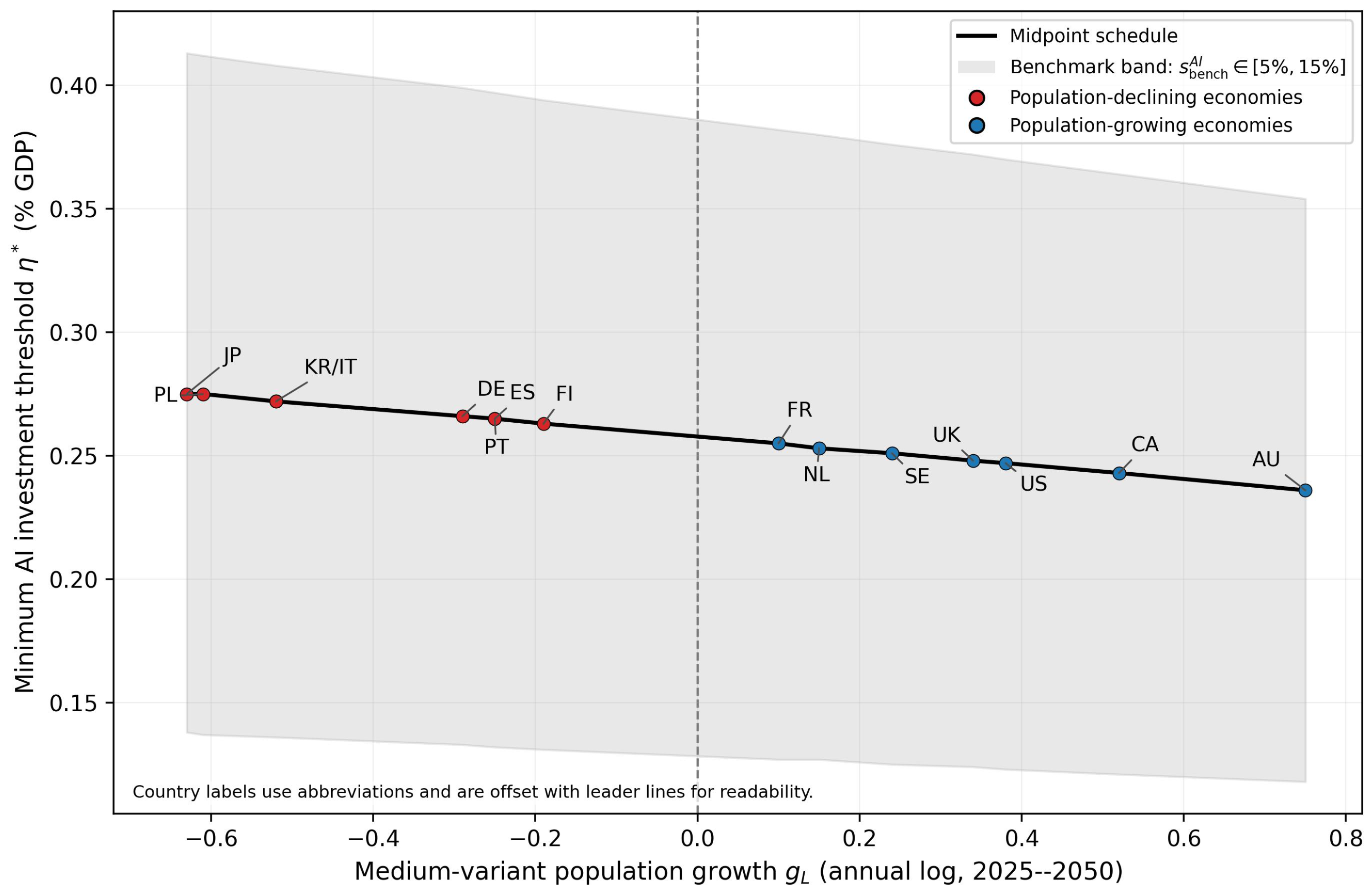
Figure 1 summarizes the cross-country threshold schedule under the midpoint benchmark.

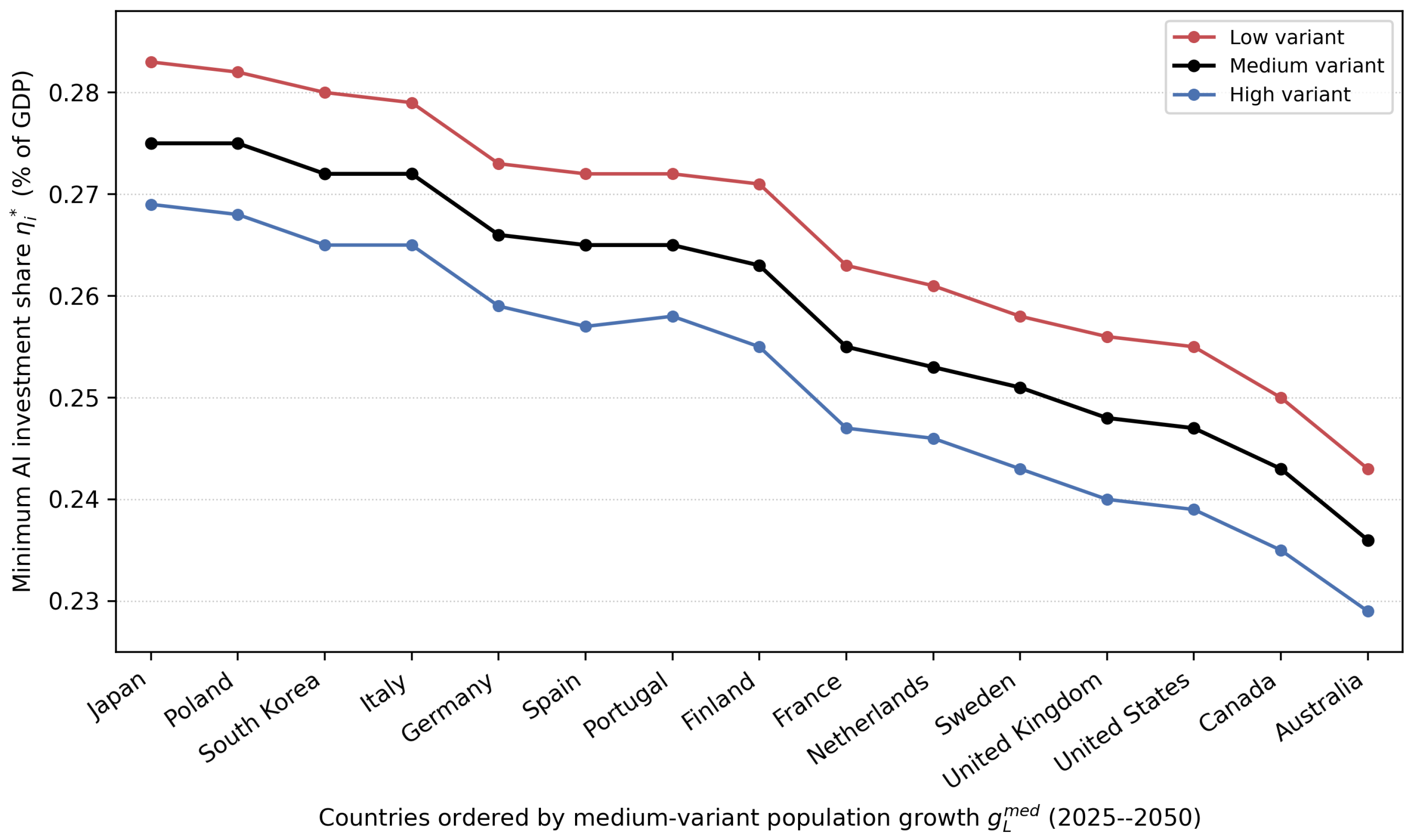
Figure 2 reports the same schedule under alternative UN WPP demographic variants.

5.3. Key Findings and Restricted Interpretation

Before presenting the individual findings, it is useful to clarify the order of robustness among the quantitative results. The most robust object is the cross-country ranking, together with the negative sign of the demographic effect. Because $s_{\mathrm{obs}}^{AI}$ is not directly observable in standard R&D statistics for most countries, the reported country-level thresholds are conditional on the common benchmark scenarios $s_{\mathrm{bench}}^{AI}$ and the associated benchmark ratio ${\overline{\chi }}^{\mathrm{bench}}$. The limited observed anchors and the maintained benchmark scenarios introduced above motivate the full 15-country exercise.

Table 6. Sensitivity analysis for Japan, Australia, and Poland under the midpoint benchmark $s_{\mathrm{bench}}^{AI}=10\%$.

Scenario	Japan ${\mathit{\eta }}^{*}$ (% GDP)	Australia ${\mathit{\eta }}^{*}$ (% GDP)	Poland ${\mathit{\eta }}^{*}$ (% GDP)
Panel A. Level-moving and policy-accounting scenarios
Baseline ($\beta =1.6$, $\varphi =0.25$, $\theta =0.40$, $\psi =0.30$, ${\delta }_R=0.15$, $\overline{\chi }=58.28$)	0.275	0.236	0.275
High AI elasticity ($\psi =0.45$)	0.269	0.243	0.269
Low AI elasticity ($\psi =0.15$)	0.293	0.214	0.292
High depreciation (${\delta }_R=0.20$)	0.361	0.322	0.361
Low depreciation (${\delta }_R=0.10$)	0.190	0.150	0.189
High $\overline{\chi }$ (5% benchmark AI share in mean GERD)	0.138	0.118	0.137
Low $\overline{\chi }$ (15% benchmark AI share in mean GERD)	0.413	0.354	0.412
Weaker population scale effect ($\kappa =0.25$)	0.266	0.247	0.266
Stronger population scale effect ($\kappa =0.75$)	0.284	0.225	0.284
Crowding out ($c=0.25$)	0.367	0.315	0.366
Crowding out ($c=0.50$)	0.551	0.472	0.550
Capital-deepening allowance ($d_K=+0.2$ pp)	0.250	0.211	0.249
Capital-deepening allowance ($d_K=+0.3$ pp)	0.237	0.198	0.237
Migration relief ($g_{migration}=+0.2$ percentage points)	0.270	0.230	0.269
Migration relief ($g_{migration}=+0.5$ percentage points)	0.261	0.222	0.261
Scenario	${\mathit{\beta }}_{\mathbf{min}}=\mathit{\varphi }\mathit{\theta }\mathit{\sigma }$	$\mathit{\beta }-{\mathit{\beta }}_{\mathbf{min}}$	Implication for ${\mathit{\eta }}^{*}$
Panel B. Admissibility diagnostics (country-invariant)
Lower local feedback ($\theta =0.20$, so $\omega =\theta \sigma =0.10$)	0.025	1.58	Unchanged relative to Panel A baseline
Higher local feedback ($\theta =0.80$, so $\omega =\theta \sigma =0.40$)	0.100	1.50	Unchanged relative to Panel A baseline
Higher human-capital elasticity ($\varphi =0.40$)	0.080	1.52	Unchanged relative to Panel A baseline
Lower stepping-on-toes ($\beta =0.40$)	0.050	0.35	Unchanged relative to Panel A baseline
Knife-edge admissibility ($\beta ={\beta }_{min}=0.05$)	0.050	0.00	No finite stable cutoff
Instability illustration ($\beta =0.04$)	0.050	$-0.01$	No finite stable cutoff

Note: Panel A reports country-specific threshold levels for the three contrast cases discussed in the text. Panel B reports admissibility diagnostics that are common across countries because Equation (15) does not depend on $\theta$, $\varphi$, or $\beta$ once the stability condition holds. Poland nearly coincides with Japan in GDP-point space because their projected population-growth rates are very similar; their policy contrast emerges after dividing by country-specific GERD in the country-level threshold comparison.

and Figure 3 show that this normalization remains the largest source of level variation. A common rescaling of $\overline{\chi }$ shifts all country thresholds proportionally, so the level and the slope magnitude in GDP space are not normalization-invariant, whereas the ranking is. Cross-country comparisons of the level of ${\eta }^{*}$ should, therefore, be treated cautiously.

Four results are worth highlighting.

First, the minimum AI investment share is highest in the fastest-declining economies, exactly as Corollary 1 predicts. Under the common benchmark scenario, Japan and Poland sit near the top of the ranking, South Korea and Italy are close behind, and Australia lies near the bottom. For two economies i and j with equal parameters except population growth rates $g_{L,i}<g_{L,j}$,

$${\eta }_i^{*}-{\eta }_j^{*}=-{\displaystyle \frac{\kappa }{\psi \overline{\chi }}}(g_{L,i}-g_{L,j})>0.$$

(18)

Under the common benchmark scenario, the cross-country spread is entirely driven by differences in demographic dynamics—a direct consequence of the theorem rather than an independent empirical finding.

Second, the benchmark normalization $s_{\mathrm{bench}}^{AI}$ matters strongly for the level. The maintained benchmark scenarios define $s_{\mathrm{bench}}^{AI}\in \{5\%,10\%,15\%\}$, and the country-level threshold results show that moving from $s_{\mathrm{bench}}^{AI}=5\%$ to $s_{\mathrm{bench}}^{AI}=15\%$ triples every country’s threshold mechanically, without changing the cross-country ordering because each cutoff is multiplied by the same factor. By construction, these are maintained benchmark scenarios rather than observed country values.

Third, the UN WPP 2024 high and low variants shift all levels in the expected direction. In the low population variant, the required cutoff rises for every country, whereas in the high population variant, it falls for every country. Population-scenario uncertainty, therefore, matters quantitatively, but it does not alter the main qualitative message of this paper.

Fourth, the GDP-point dispersion in ${\eta }_i^{*}$ is numerically modest but economically non-trivial once it is mapped into existing research bases. The midpoint thresholds span only $0.236\%$ to $0.275\%$ of GDP, yet GERD/GDP itself ranges from about $1.39\%$ to $5.21\%$ across the sample. The accounting ratio $s_i^{\mathrm{req}}={\eta }_i^{*}/m_i$, therefore, reflects both the numerator ${\eta }_i^{*}$ and the denominator $m_i$. Under the midpoint benchmark $s_{\mathrm{bench}}^{AI}=10\%$, South Korea and the United States map the conditional threshold into only about 5–$7\%$ of current GERD, whereas Italy, Poland, and Spain map it into roughly 18–$20\%$. The economically relevant contrast is, therefore, better read in $s_i^{\mathrm{req}}$ than in the raw GDP-point range alone. These contrasts are accounting statements about the maintained mapping, not theorem-level claims about the optimal internal composition of R&D.

A complementary perspective on the threshold levels is available for the three economies with direct empirical anchors. Using the observed anchors $s_{\mathrm{obs}}^{AI}$ reported above rather than the common midpoint benchmark $s_{\mathrm{bench}}^{AI}=10\%$ implies ${\overline{\chi }}^{\mathrm{obs}}\approx 42$ for the United States, ${\overline{\chi }}^{\mathrm{obs}}\approx 55$ for Japan, and ${\overline{\chi }}^{\mathrm{obs}}\approx 77$ for the EU27 aggregate. These values shift the zero-demography benchmark component ${\delta }_R/\overline{\chi }$ to approximately $0.36\%$, $0.27\%$, and $0.20\%$ of GDP, respectively. Once each country’s demographic term is added, the U.S. and Japan thresholds remain of the same order of magnitude as under the common benchmark scenario, while the EU27 anchor points to a somewhat lower benchmark level. These levels are conditional on the Fonteneau et al. (2025) measurement framework and carry its limitations, but they suggest that the order-of-magnitude content of the benchmark is not sensitive to whether one uses $s_{\mathrm{bench}}^{AI}$ or the best available observed anchors $s_{\mathrm{obs}}^{AI}$ where those exist.

5.4. Sensitivity Analysis

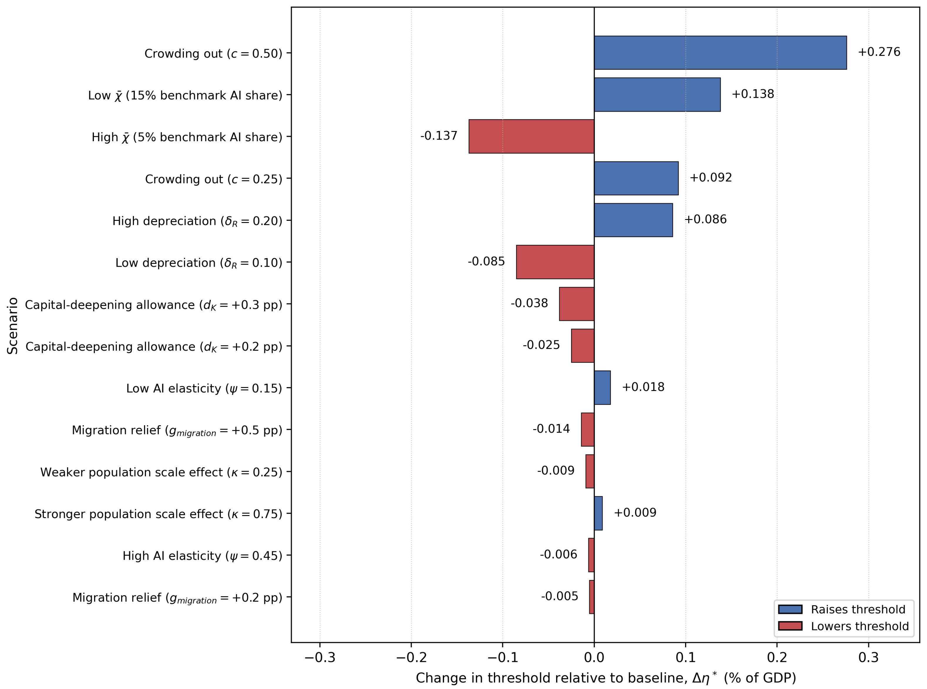
Table 6 extends the sensitivity exercise beyond Japan to Australia and Poland. Australia is the sample’s low-threshold case and still has positive population growth. Poland, by contrast, combines strong demographic pressure with a comparatively thin research base. Together they provide a useful contrast to Japan’s high-R&D benchmark. The table groups the experiments into level-moving parameters ($\psi$, ${\delta }_R$, $\overline{\chi }$, $\kappa$), fiscal transmission (c, $d_K$), local human-capital diagnostics ($\theta$, $\varphi$, $\beta$), and a mechanical demographic extension (migration). Figure 3 retains Japan as the focal visual benchmark and plots the Japan column of Panel A as a tornado chart.

Figure 3 orders the level-moving scenarios by the absolute size of their deviation from Japan’s baseline threshold of $0.275\%$ of GDP; Japan is plotted because it lies near the upper end of the sample distribution, while Table 6 shows the same scenarios for Australia and Poland.

Five points stand out. First, uncertainty about $\overline{\chi }$ remains the largest source of level variation in all three cases, which is why the benchmark window in $s_{\mathrm{bench}}^{AI}$ is shown explicitly in the benchmark-scenario and country-level threshold results, and graphically in Figure 1. Within the maintained range, ${\delta }_R$ is the next most important structural level driver, whereas the fiscal-transmission wedges c and $d_K$ generate sizable but mechanically interpretable shifts.

Second, Poland tracks Japan closely in GDP-point space because the two economies have very similar projected population-growth rates. The sharper policy contrast between them, therefore, comes mainly from the denominator in $s_i^{\mathrm{req}}={\eta }_i^{*}/m_i$: Poland’s lower GERD intensity makes a similar GDP-point threshold much more demanding as a share of existing research expenditure.

Third, Australia shows that the sensitivity exercise is not specific to shrinking economies. Parameters that move only the intercept of Equation (15), such as ${\delta }_R$, $\overline{\chi }$, crowding out, or capital deepening, shift all three cases in the same direction. By contrast, parameters that enter through the demographic term $-(\kappa /\psi )g_L$ have sign-sensitive level effects: Stronger population scale effects or lower AI elasticity raise the threshold in Japan and Poland, where $g_L<0$, but lower it in Australia, where $g_L>0$.

Fourth, migration relief and capital deepening remain quantitatively meaningful but transparent accounting wedges. A common $+0.2$ or $+0.5$ percentage-point migration contribution lowers the threshold by the same absolute amount in all three countries, while a given capital-deepening allowance subtracts the same GDP-point amount from each country’s cutoff. Crowding out works differently: It scales up the gross fiscal requirement proportionally, so high-threshold economies retain higher gross needs in absolute terms.

Fifth, $\theta$, $\varphi$, and $\beta$ matter mainly through admissibility rather than through the level of Equation (15). This is because Equation (15) depends on these parameters only through the admissibility condition $\beta >\varphi \theta \sigma$; once that condition is satisfied, they cancel out of the threshold formula entirely. Panel B shows that once the stability condition is satisfied, these parameters do not alter the conditional spending formula. The local human-capital and congestion parameters, therefore, govern whether the benchmark is well behaved, not the level of the cutoff itself.

6. Discussion

6.1. Relation to the Existing Literature

The quantitative exercise helps position the paper more sharply within the existing literature. Relative to the semi-endogenous growth tradition initiated by Jones (1995), the contribution here is not a new claim that weaker population growth slows idea production in general, but an explicit threshold formula for the AI-designated research intensity required to offset that pressure on a balanced-growth path. Relative to Growiec (2022), the present framework does not treat research capital as a generic engine of growth. Instead, it interprets the additional stock as AI-designated research capital and asks what minimum share is needed when demographic conditions deteriorate. Relative to empirical threshold studies such as Wen et al. (2025), the contribution is structural rather than statistical. Their threshold is a reduced-form breakpoint in observed data, whereas Equation (15) maps demographic pressure, depreciation, and research transmission into a conditional investment cutoff that can be compared across countries under a common normalization.

The numerical findings also clarify what is and is not robust in that contribution. The most stable quantitative objects are the sign of the demographic slope and the resulting cross-country ranking under a common normalization. By contrast, the level of the cutoff in GDP space remains conditional on the maintained benchmark ratio $\overline{\chi }$. This is why the paper interprets the reported levels as conditional benchmarks rather than unconditional policy targets. Appendix C sharpens that interpretation further. It shows that the household Euler structure is not what drives the threshold result, while production-side physical capital matters only to the extent that capital deepening contributes an additional wedge to current per capita growth.

6.2. Policy Interpretation

Four policy implications follow from the benchmark. First, the quantitative results support a differentiated reading across country groups rather than a common OECD-wide target. In research-rich but demographically pressured economies such as Japan, Germany, and South Korea, the midpoint thresholds correspond to roughly 5–$9\%$ of existing GERD, so the immediate priority is less the creation of an entirely new research base than the more efficient redirection and transmission of existing research budgets toward AI-designated capital. In lower-pressure, research-rich economies such as the United States and the United Kingdom, the implied burdens are also moderate, which suggests that incremental top-ups and portfolio shifts may be sufficient. By contrast, in Italy, Poland, and Spain, the same GDP-point thresholds map into roughly 18–$20\%$ of current GERD. For that group, stepwise expansion of the research base itself is likely to be a precondition for meeting the benchmark without excessive displacement of other research activity.

Second, migration policy and AI-research effort act as partial substitutes in the benchmark accounting of Equation (15). In Table 6, a $0.2$ percentage-point improvement in the effective labor-force term lowers the implied threshold by about $0.005$ percentage points of GDP, while a $0.5$ percentage-point improvement lowers it by about $0.014$ percentage points. Interpreted cautiously, this means that policies that durably improve net migration, labor-force attachment, or skill retention can reduce the additional AI effort otherwise required. The relevant lesson is not that migration can replace innovation policy, but that demographic, education, and AI policies should be coordinated because they operate on the same threshold through different margins.

Third, the economically relevant object is net AI research capital rather than gross public outlays alone. Under the reduced-form crowding-out extension in Table 6, a $25\%$ displacement rate raises Japan’s gross requirement from $0.275\%$ to $0.367\%$ of GDP, and a $50\%$ displacement rate raises it to $0.551\%$. This points to a design principle more than a single instrument ranking: Policies that crowd in or preserve private AI-designated R&D are likely to be more effective than schemes that merely relabel existing activity. Tax credits, matching grants, procurement-linked co-investment, and shared research infrastructure may, therefore, be more fiscally effective than stand-alone subsidies when the objective is to maximize net AI research capital.

Fourth, the benchmark points to an institutional role for the OECD. Rather than promoting a single OECD-wide AI-spending ratio, a more useful practice would be to publish country-specific benchmark ranges that combine demographic projections, GERD intensity, and the evolving OECD/EC AI-measurement framework. Such a dashboard would not deliver optimal policy on its own, but it would translate a common methodology into differentiated national benchmarks and make cross-country monitoring more transparent.

These implications are policy-relevant precisely because the benchmark remains transparent. The paper does not solve for an optimal portfolio of subsidies, migration, and education policy. It instead provides a tractable way to translate demographic pressure into an approximate scale of AI-designated research effort and to identify where complementary policies can relax that requirement.

6.3. Limitations

The benchmark is deliberately narrow in scope. It is not a forecasting equation, and it is not a structural estimate of the optimal internal composition of R&D. The quantitative exercise fixes the long-run ratio $\overline{\chi }\equiv Y/R$ externally and uses the current OECD/EC evidence on AI-designated R&D shares to anchor a plausible normalization window. As a result, the reported levels should be read as conditional benchmarks rather than point predictions. The model also uses total population growth as a broad proxy for research scale in the baseline and suppresses transitional dynamics that would matter in a richer quantitative model.

A second limitation is that the present closure remains intentionally incomplete. Although Appendix C shows how physical capital accumulation modifies the threshold logic in a transparent way, the paper does not estimate a fully closed general equilibrium with endogenous savings, capital accumulation, and country-specific research-capital transmission. The benchmark is, therefore, best interpreted as isolating one margin of adjustment—AI-designated research intensity—rather than as a complete quantitative model of growth under aging.

6.4. Directions for Future Research

Four extensions are especially natural. The first is measurement: As the OECD/EC framework of Fonteneau et al. (2025) matures and national statistical offices begin to report AI-designated R&D more systematically, the common normalization used here can be replaced with country-specific values of $\overline{\chi }$. The second is closure: A capital-augmented general equilibrium with explicit household saving would allow the benchmark ratio $Y/R$ to be jointly determined rather than externally fixed. The third is demography: Alternative scale proxies, labor-force composition, and migration dynamics could be incorporated more explicitly than in the current reduced-form mapping. The fourth is empirical validation: Future work could compare the benchmark more directly with observed country-level AI-investment programs, crowding-out patterns, and realized productivity outcomes.

7. Conclusions

This paper derives a transparent threshold formula for the minimum AI-designated research intensity consistent with non-negative per capita growth on a balanced-growth path under demographic decline. In the benchmark, faster population decline raises the required AI share linearly, and the resulting cross-country ranking is stable under common rescalings of the normalization. Applied to 15 illustrative OECD economies, the formula implies a narrow GDP-point range but materially different burdens once the threshold is expressed relative to existing national research bases.

The policy reading is, therefore, differentiated rather than uniform. In research-rich economies under stronger demographic pressure, the main task is to raise the AI-designated share and transmission efficiency of existing research budgets. In lower-pressure research leaders, moderate top-ups may be sufficient. In thinner-base systems such as Italy, Poland, and Spain, expansion of the research base itself is likely to be a necessary complement to AI-targeted spending. Migration and labor-force policies can also relax the implied AI requirement, while subsidy design should focus on maximizing net AI research capital rather than gross outlays alone.

The reported levels remain conditional benchmarks, not forecasts or structural policy optima. Even so, the benchmark is informative because it makes the demographic slope of the minimum AI requirement explicit and portable across countries. Until richer country-specific AI-R&D statistics and a fuller general-equilibrium closure become available, the threshold formula provides a tractable, demographically grounded benchmark for economies confronting both population decline and the transition to AI-intensive growth.

References

1. Abeliansky, A. L., & Prettner, K. (2023). Automation and population growth: Theory and cross-country evidence. Journal of Economic Behavior & Organization, 208, 345–358. [Google Scholar] [CrossRef] [Scilit]
2. Acemoglu, D., Autor, D., Hazell, J., & Restrepo, P. (2022). Artificial intelligence and jobs: Evidence from online vacancies. Journal of Labor Economics, 40(S1), S293–S340. [Google Scholar] [CrossRef] [Scilit]
3. Acemoglu, D., & Restrepo, P. (2022). Demographics and automation. The Review of Economic Studies, 89(1), 1–44. [Google Scholar] [CrossRef] [Scilit]
4. Aghion, P., Jones, B. F., & Jones, C. I. (2019). Artificial intelligence and economic growth. In A. Agrawal, J. Gans, & A. Goldfarb (Eds.), The economics of artificial intelligence: An agenda (pp. 237–282). University of Chicago Press. [Google Scholar] [CrossRef] [Scilit]
5. Almeida, D., Naudé, W., & Sequeira, T. N. (2024). Artificial intelligence and the discovery of new ideas: Is an economic growth explosion imminent? IZA discussion paper, No. 16766. Available online: https://www.iza.org/publications/dp/16766/artificial-intelligence-and-the-discovery-of-new-ideas-is-an-economic-growth-explosion-imminent (accessed on 25 March 2025).
6. Babina, T., Fedyk, A., He, A., & Hodson, J. (2024). Artificial intelligence, firm growth, and product innovation. Journal of Financial Economics, 151, 103745. [Google Scholar] [CrossRef] [Scilit]
7. Ben-Porath, Y. (1967). The production of human capital and the life cycle of earnings. Journal of Political Economy, 75(4), 352–365. [Google Scholar] [CrossRef] [Scilit]
8. Bloom, N., Jones, C. I., Van Reenen, J., & Webb, M. (2020). Are ideas getting harder to find? American Economic Review, 110(4), 1104–1144. [Google Scholar] [CrossRef] [Scilit]
9. Bloom, N., Schankerman, M., & Van Reenen, J. (2013). Identifying technology spillovers and product market rivalry. Econometrica, 81(4), 1347–1393. [Google Scholar] [CrossRef] [Scilit]
10. Brynjolfsson, E., Li, D., & Raymond, L. R. (2025). Generative AI at work. The Quarterly Journal of Economics, 140(2), 889–942. [Google Scholar] [CrossRef] [Scilit]
11. Brynjolfsson, E., & McAfee, A. (2014). The second machine age: Work, progress, and prosperity in a time of brilliant technologies. W. W. Norton & Company. [Google Scholar]
12. Bureau of Economic Analysis. (2024). Gross domestic product, fourth quarter and year 2023 (second estimate). Available online: https://www.bea.gov/news/2024/gross-domestic-product-fourth-quarter-and-year-2023-second-estimate (accessed on 23 June 2025).
13. Cabinet Office, Government of Japan. (2024). Annual report on national accounts for 2023 (flow accounts). Economic and Social Research Institute. Available online: https://www.esri.cao.go.jp/en/sna/data/kakuhou/files/2023/pdf/point_flow_en20241223.pdf (accessed on 18 June 2025).
14. Cabinet Office, Government of Japan. (2025). Artificial intelligence basic plan. Cabinet Decision. Available online: https://www8.cao.go.jp/cstp/ai/ai_plan/aiplan_eng_20260116.pdf (accessed on 2 January 2026).
15. Cockburn, I. M., Henderson, R., & Stern, S. (2019). The impact of artificial intelligence on innovation: An exploratory analysis. In A. Agrawal, J. Gans, & A. Goldfarb (Eds.), The economics of artificial intelligence: An agenda (pp. 115–146). University of Chicago Press. [Google Scholar] [CrossRef] [Scilit]
16. Czarnitzki, D., Fernández, G. P., & Rammer, C. (2023). Artificial intelligence and firm-level productivity. Journal of Economic Behavior & Organization, 211, 188–205. [Google Scholar] [CrossRef] [Scilit]
17. David, P. A., Hall, B. H., & Toole, A. A. (2000). Is public R&D a complement or substitute for private R&D? A review of the econometric evidence. Research Policy, 29(4–5), 497–529. [Google Scholar] [CrossRef] [Scilit]
18. European Central Bank. (2026). ECB data portal: US dollar/Euro ECB reference exchange rate, annual average. Available online: https://data.ecb.europa.eu/data/concepts/united-states-dollar?tags_array%5B0%5D=United+States+dollar (accessed on 31 March 2026).
19. European Commission. (2024). European artificial intelligence act comes into force. Available online: https://digital-strategy.ec.europa.eu/en/news/european-artificial-intelligence-act-comes-force (accessed on 28 February 2026).
20. Eurostat. (2024). EU spent EUR 381.4 billion on R&D in 2023. Available online: https://ec.europa.eu/eurostat/web/products-eurostat-news/w/ddn-20241211-2 (accessed on 12 July 2025).
21. Fonteneau, F., Mollins, J., Marchi, S., Russo, L., Gentaz, A., Daoud, M., & André, A.-A. (2025). Advancing the measurement of investments in artificial intelligence. OECD Artificial intelligence papers, No. 47. OECD. [Google Scholar] [CrossRef] [Scilit]
22. Galor, O., & Weil, D. N. (2000). Population, technology, and growth: From malthusian stagnation to the demographic transition and beyond. American Economic Review, 90(4), 806–828. [Google Scholar] [CrossRef] [Scilit]
23. González, X., & Pazó, C. (2008). Do public subsidies stimulate private R&D spending? Research Policy, 37(3), 371–389. [Google Scholar] [CrossRef] [Scilit]
24. Growiec, J. (2022). R&D capital: An engine of growth. Economics Letters, 217, 110703. [Google Scholar] [CrossRef] [Scilit]
25. Hall, R. E., & Jones, C. I. (1999). Why do some countries produce so much more output per worker than others? The Quarterly Journal of Economics, 114(1), 83–116. [Google Scholar] [CrossRef] [Scilit]
26. Jones, C. I. (1995). R&D-based models of economic growth. Journal of Political Economy, 103(4), 759–784. [Google Scholar] [CrossRef] [Scilit]
27. Jones, C. I. (2022). The past and future of economic growth: A semi-endogenous perspective. Annual Review of Economics, 14(1), 125–152. [Google Scholar] [CrossRef] [Scilit]
28. Klenow, P. J., & Rodríguez-Clare, A. (1997). The neoclassical revival in growth economics: Has it gone too far? In B. S. Bernanke, & J. J. Rotemberg (Eds.), NBER macroeconomics annual 1997 (Vol. 12, pp. 73–114). MIT Press. [Google Scholar] [CrossRef]
29. Korinek, A., & Stiglitz, J. E. (2021). Artificial intelligence, globalization, and strategies for economic development. NBER working paper, No. 28453. NBER. [Google Scholar] [CrossRef] [Scilit]
30. Kortum, S. S. (1997). Research, patenting, and technological change. Econometrica, 65(6), 1389–1419. [Google Scholar] [CrossRef] [Scilit]
31. Lach, S. (2002). Do R&D subsidies stimulate or displace private R&D? Evidence from Israel. The Journal of Industrial Economics, 50(4), 369–390. [Google Scholar] [CrossRef] [Scilit]
32. Lucas, R. E., Jr. (1988). On the mechanics of economic development. Journal of Monetary Economics, 22(1), 3–42. [Google Scholar] [CrossRef] [Scilit]
33. Minniti, A., & Venturini, F. (2017). The long-run growth effects of R&D policy. Research Policy, 46(1), 316–326. [Google Scholar] [CrossRef] [Scilit]
34. Nelson, R. R., & Phelps, E. S. (1966). Investment in humans, technological diffusion, and economic growth. American Economic Review, 56(1/2), 69–75. [Google Scholar]
35. OECD. (2025). Main science and technology indicators (MSTI database). Available online: https://www.oecd.org/en/data/datasets/main-science-and-technology-indicators.html (accessed on 31 March 2026).
36. Presidency of the French Republic. (2025). Make France an AI powerhouse. Available online: https://www.elysee.fr/en/emmanuel-macron/2025/02/11/make-france-an-ai-powerhouse (accessed on 31 March 2026).
37. Prime Minister of Canada. (2024). Securing Canada’s AI advantage. Available online: https://www.pm.gc.ca/en/news/news-releases/2024/04/07/securing-canadas-ai (accessed on 3 April 2025).
38. Romer, P. M. (1990). Endogenous technological change. Journal of Political Economy, 98(5), S71–S102. [Google Scholar] [CrossRef] [Scilit]
39. Strulik, H. (2024). Long-run economic growth despite population decline. Journal of Economic Dynamics and Control, 168, 104943. [Google Scholar] [CrossRef] [Scilit]
40. United Nations, Department of Economic and Social Affairs, Population Division. (2024). World population prospects 2024. Available online: https://population.un.org/wpp/ (accessed on 15 May 2025).
41. Vollrath, D. (2020). Fully grown: Why a stagnant economy is a sign of success. University of Chicago Press. [Google Scholar] [CrossRef] [Scilit]
42. Wallsten, S. J. (2000). The effects of government-industry R&D programs on private R&D: The case of the small business innovation research program. The RAND Journal of Economics, 31(1), 82–100. [Google Scholar] [CrossRef] [Scilit]
43. Wen, H., Shang, J., & Nghiem, X.-H. (2025). Does artificial intelligence matter for the population aging-inclusive growth nexus? International evidence. Telecommunications Policy, 49(4), 102932. [Google Scholar] [CrossRef] [Scilit]
Figure 1. Minimum artificial intelligence (AI) investment threshold η * against population growth g L (2025–2050). Country points are plotted under the midpoint benchmark s bench A I = 10 % ; the shaded band spans s bench A I ∈ [ 5 % , 15 % ] . Labels use country abbreviations and colors distinguish population-declining from population-growing economies. Labels are offset for readability, but data points are not jittered; South Korea and Italy coincide under the midpoint benchmark and are, therefore, labeled jointly as KR/IT.
Economies 14 00176 g001
Figure 2. United Nations World Population Prospects (UN WPP) demographic-scenario sensitivity of η i * . Countries are ordered by medium-variant population growth g L m e d ; the low, medium, and high variants shift the schedule in parallel under the midpoint benchmark s bench A I = 10 % . For policymakers, this means that alternative demographic scenarios mainly move the level of the benchmark rather than the overall demographic pattern it encodes. This statement concerns changes in the UN WPP scenario holding the total-population scale proxy fixed; Appendix B shows that changing the scale proxy itself can alter some mid-table rankings.
Economies 14 00176 g002
Figure 3. Sensitivity of Japan’s conditional threshold η * to the level-moving scenarios in Panel A of Table 6. Bars show Δ η * relative to the baseline of 0.275 % of GDP, ordered by absolute magnitude. The κ range captures how stronger or weaker population-scale effects steepen or flatten the demographic threshold schedule.
Economies 14 00176 g003