Article

The Interaction Between Fiscal and Monetary Policy Under Political Turmoil in Myanmar: New Keynesian DSGE Model

Faculty of Economics, Chiang Mai University, Chiang Mai 50200, Thailand
*
Author to whom correspondence should be addressed.
Economies 2026, 14(5), 157; https://doi.org/10.3390/economies14050157
Submission received: 24 February 2026 / Revised: 19 March 2026 / Accepted: 2 April 2026 / Published: 4 May 2026

Abstract

This paper examines the interaction between fiscal and monetary policies in Myanmar under ongoing political and economic uncertainty. We estimate a small open-economy New Keynesian DSGE model using Bayesian methods, combining the Kalman filter with Markov Chain Monte Carlo sampling on quarterly data from 2013Q1 to 2022Q1. The results show a persistent regime of monetary and fiscal policy conflict. While the central bank follows an active anti-inflationary interest rate rule that satisfies the Taylor principle, fiscal policy shows weak responsiveness to public debt, providing limited fiscal backing for monetary stabilization. As a result, monetary tightening aimed at controlling inflation exacerbates fiscal stress through the debt-service channel, undermining the overall effectiveness of macroeconomic stabilization. Political instability emerges as a key structural driver of macroeconomic fragility. Political shocks are highly persistent and are transmitted primarily through increases in the country risk premium, accounting for more than 50% of real exchange rate volatility and generating exchange rate depreciation, higher inflation, and output contraction. Overall, the findings indicate that monetary tightening alone is insufficient to restore macroeconomic stability in fragile and conflict-affected economies. Credible fiscal adjustment and improvements in political stability are necessary to contain external vulnerabilities and restore the effectiveness of monetary policy.

1. Introduction

Myanmar’s macroeconomic environment experienced a profound structural break in 2021. Following nearly a decade of gradual economic liberalization and reintegration into the global economy between 2011 and 2020, the country was hit by two exceptional shocks: the COVID-19 pandemic and the military-led political transition in February 2021. The macroeconomic consequences were immediate and severe. Real output declined sharply, the domestic currency depreciated rapidly, and inflation rose above 10 percent. While international institutions attribute this downturn to social unrest, trade disruptions, capital outflows, and economic sanctions (World Bank, 2022), the structural mechanisms governing Myanmar’s post-2021 macroeconomic dynamics remain poorly understood.
In particular, the interaction between fiscal and monetary policies under heightened political uncertainty has not been systematically analyzed. Existing studies on Myanmar tend to examine fiscal or monetary policy in isolation, abstracting from their joint determination and from the role of political instability. This omission is especially consequential in fragile and conflict-affected economies, where weak institutions and limited policy credibility may fundamentally alter standard policy transmission mechanisms. Understanding how fiscal and monetary authorities interact—and how political turmoil disrupts that interaction—is therefore not merely an academic question but a precondition for any credible stabilization strategy in Myanmar.
The fiscal–monetary interaction literature establishes that macroeconomic stability requires regime consistency between the two policy authorities. Leeper (1991) demonstrates that intertemporal budget balance must be ensured by at least one authority, and that when fiscal adjustment is weak, monetary policy may remain formally active yet become constrained in practice. Empirical evidence from emerging and transition economies supports this view. Vasiljev (2018) finds that weak and unpredictable fiscal behavior in Serbia forces the central bank into a defensive stabilization stance, limiting policy effectiveness despite formal adherence to inflation-targeting principles. Applying these frameworks to low-income and fragile states requires further adaptation, as fiscal policy in such economies is often acyclical or procyclical due to institutional constraints (Talvi & Végh, 2005), while monetary transmission is weakened by shallow financial markets and bank-dependent credit systems, conditions that are particularly pronounced across the CLMV region (Fan & Lynn, 2024b). Within Myanmar specifically, existing studies focus primarily on the long-run growth and poverty-reducing effects of public investment, abstracting from political instability and short-run stabilization dynamics (Fan & Lynn, 2024a).
Fiscal and monetary factors alone, however, do not fully explain the sudden-stop nature of Myanmar’s 2021 crisis. The growing literature links political instability to macroeconomic volatility through financial channels. Reduced-form evidence shows that political conflict depresses growth and raises volatility (Acemoglu et al., 2003), while structural models demonstrate that political instability increases sovereign risk premia and external financing costs (Cuadra & Sapriza, 2008; Singh et al., 2015). Concurrently, recent structural analyses document that heightened political and institutional uncertainty significantly amplifies country risk premia, generating severe capital outflows and exchange rate volatility in frontier economies (Caldara et al., 2019; Hammoudeh, 2024). Recent DSGE evaluations further show that when fiscal authorities act passively toward debt stabilization, the full burden of inflation control falls on monetary policy, often producing destabilizing stagflationary consequences (Barrie & Jackson, 2022; Lakhchen, 2025).
Despite these parallel advances, the two strands of the literature have remained largely separate. Studies of fiscal–monetary conflict treat country risk premia as exogenous stochastic processes (Justiniano & Preston, 2010; Schmitt-Grohé & Uribe, 2003), while studies of political risk rely predominantly on reduced-form methods that cannot identify structural transmission mechanisms (Acemoglu et al., 2003; Cuadra & Sapriza, 2008). No existing study—to our knowledge—has structurally endogenized political instability within a monetary–fiscal conflict framework and estimated it on data spanning an acute political crisis in a frontier economy. This paper closes that gap.
The main contribution of this paper is methodological: we endogenize the country risk premium by mapping an observed, high-frequency political instability index directly into the risk premium process via a structural parameter χ, estimated through Bayesian methods within a small open-economy New Keynesian framework, building on Galí and Monacelli (2005) and Justiniano and Preston (2010). Unlike standard applications that treat the risk premium as a black-box exogenous shock, our specification in Equation (9) establishes a disciplined, theory-consistent link between the political process and external financing costs. This allows, for the first time in the Myanmar context, a structural quantification of how political turmoil propagates through the exchange rate into inflation and output—a transmission channel that reduced-form approaches cannot separately identify. The posterior estimate of χ is strictly positive across all robustness specifications, providing clear empirical validation of this channel rather than merely assuming its existence.
Building on this methodological foundation, the paper delivers two further contributions. Empirically, we provide the first Bayesian DSGE estimation for Myanmar spanning both the pre- and post-2021 transition, producing quantitative evidence that the post-coup collapse was driven overwhelmingly by aggregate demand contraction—consistent with a sudden stop in consumption and investment—rather than a supply-side productivity slowdown. This finding directly advances the nascent empirical literature on CLMV economies (Fan & Lynn, 2024b) by providing a structurally identified decomposition of the crisis that existing reduced-form studies cannot offer. From a policy perspective, the paper jointly identifies a regime of active monetary policy and weak fiscal discipline—a configuration that Leeper (1991) defines as placing the full burden of price-level determination on the fiscal authority—and demonstrates that this regime, when amplified by persistent political risk, generates a self-reinforcing stagflationary spiral. Political instability is thus not merely a background condition but a quantitatively dominant structural driver of macroeconomic fragility, accounting for over 52 percent of real exchange rate variance in our baseline estimates.
The remainder of the paper is organized as follows. Section 2 presents the theoretical model. Section 3 describes the data, estimation strategy, and empirical results, including calibration (Section 3.1), Bayesian estimation (Section 3.2), structural parameter estimates (Section 3.3), shock volatilities and crisis dynamics (Section 3.4), impulse response analysis (Section 3.5), robustness checks (Section 3.6), and forecast error variance decomposition (Section 3.7). Section 4 discusses policy implications and limitations, and contains the conclusion.

2. Methodology

2.1. Households

The representative household maximizes expected lifetime utility (Galí, 2015), E 0 t = 0 β t C t 1 σ 1 σ N t 1 + φ 1 + φ , where C t denotes consumption, N t hours worked, β 0 , 1 the discount factor, σ > 0 the coefficient of relative risk aversion (inverse of the intertemporal elasticity of substitution), and φ > 0 the inverse Frisch elasticity. The household’s intertemporal budget constraint is as follows:
P t C t + B t 1 + i t 1 B t 1 + W t N t + Π t T t ,
where P t is the price level, B t represents one-period nominal bond holdings purchased at t and paying 1 + i t 1 at t + 1, W t the nominal wage, Π t profits rebated to households, and T t lump-sum taxes. Gross inflation is denoted as π t + 1 P t + 1 / P t . The first-order condition with respect to bond holdings yields the standard consumption Euler equation, then we get the consumption Euler equations, 1 = β E t C t + 1 C t σ 1 + i t Π t + 1 , where σ denotes the inverse of the intertemporal elasticity of substitution, i t is the nominal interest rate (Woodford, 2003), and π t + 1 is the inflation rate. The intratemporal condition equating the marginal rate of substitution to the real wage is W t P t = C t σ N t φ .
Log-linearizing this condition around a zero-inflation steady state produces the dynamic relationship for consumption demand: c t ^ = E t c t + 1 ^ 1 σ i t ^ E t π t + 1 ^ + ε c , t , where hats denote log deviations from steady state and ε c , t captures exogenous shifts in desired intertemporal consumption growth (Clarida et al., 1999). Current consumption depends on expected future consumption minus the real interest rate gap, scaled by the elasticity 1 / σ .

2.2. Aggregate Demand (IS Curve)

In a small open-economy setting, goods market clearing maps aggregate demand to output via Y t =   C t +   G t . Following Galí and Monacelli (2005), we substitute the consumption Euler equation into the log-linearized market clearing condition to derive the open-economy IS curve:
y t ^ = E t y t + 1 ^ 1 σ i ^ t E t π t + 1 ^ + ψ q t ^ + ε y , t ,
where y ^ t denotes the output gap, i ^ t the deviation of the nominal interest rate from its steady-state value, E t π ^ t + 1 the rationally expected inflation rate one period ahead, q ^ t the real exchange rate (an increase denotes a real depreciation), ψ > 0 captures the sensitivity of aggregate demand to external conditions via the real exchange rate channel, and ε y , t is an exogenous aggregate demand shock. Note that i ^ t enters here through the real interest rate term i ^ t E t π ^ t + 1 , which governs intertemporal consumption decisions; its full characterization as a policy instrument is given by the monetary policy rule in Equation (3).

2.3. Aggregate Supply (Firms)

The supply side of the economy is characterized by a continuum of monopolistically competitive firms, indexed by j 0 , 1 ,   Y t j = A t N t j where A t is aggregate productivity. Prices are sticky à la Calvo (1983). In each period, a fraction 1 θ of firms can reset prices optimally, while the remaining fraction θ keep prices unchanged.

2.4. Open-Economy New Keynesian Phillips Curve

Solving the price-setting problem and log-linearizing around a zero-inflation steady state yields a forward-looking Phillips curve. In an open-economy environment—where CPI inflation is influenced by external prices and exchange rate movements (Galí & Monacelli, 2005)—domestic inflation dynamics can be written as
π t ^ = β E t π t + 1 ^ + κ y t ^ + α q q t ^ + ϵ π , t ,
where κ > 0 measures the sensitivity of inflation to domestic economic activity, α q > 0 captures exchange rate pass-through to CPI inflation, and ε π , t is a cost-push (markup) shock capturing non-demand supply disturbances.

2.5. Monetary Policy

Monetary policy follows an interest rate feedback rule of the inertial (smoothed) Taylor type. The central bank adjusts the short-term nominal policy rate in response to deviations in inflation and real activity from their targets, while allowing for partial adjustment in the policy instrument (Taylor, 1993; Clarida et al., 1999; Woodford, 2003; Galí, 2015). In log-linear form, the rule is
i t ^ = ρ i i t 1 ^ + 1 ρ i ϕ π π t ^ + ϕ y y t ^ + ϵ i , t ,
where i ^ t denotes the deviation of the nominal policy rate from its steady-state value, π ^ t is inflation (deviation from target), and y ^ t is the output gap. The parameter ρ i [ 0 , 1 captures interest-rate smoothing; ϕ π and ϕ y govern the policy response to inflation and the output gap, respectively; and ε i , t is an exogenous monetary policy shock.

On the Monetary Policy Rule and Fear of Floating in Myanmar

An important consideration in applying a standard Taylor-type rule to Myanmar concerns the phenomenon of “fear of floating,” documented by Calvo and Reinhart (2002) for developing economies. Fear of floating refers to the tendency of developing countries’ central banks to resist exchange rate fluctuations by adjusting policy interest rates in response to currency movements, effectively targeting exchange rate stability alongside or in lieu of inflation and output stabilization. Under this behavior, the central bank raises the policy rate not only when inflation exceeds its target but also when the exchange rate depreciates sharply, with the aim of preventing capital flight and currency crises. This mechanism creates an additional channel through which exchange rate movements affect interest rates and, consequently, debt-servicing costs through the debt-service channel in Equation (6).
There are three reasons why the standard Taylor rule in Equation (3) remains an appropriate specification for this paper despite Myanmar’s developing economy context. First, the Central Bank of Myanmar’s statutory mandate emphasizes inflation control as its primary objective throughout the sample period. As shown in the estimation results in Section 3.3, the posterior inflation response coefficient lies strictly above unity, consistent with this anti-inflationary orientation and satisfying the Taylor principle, indicating that the central bank systematically prioritized inflation stabilization. Second, exchange rate dynamics are not absent from the model’s monetary transmission mechanism; they enter explicitly through the UIP condition in Equation (7), the exchange rate pass-through term α q in the NKPC in Equation (2), and the country risk premium channel in Equation (9), which captures how political instability affects the exchange rate and feeds back into inflation and output. The Taylor rule therefore operates within a model environment where exchange rate pressures are transmitted through multiple structural channels, even if the rule itself does not include an explicit exchange rate term. Third, augmenting the Taylor rule with an exchange rate response term would require identifying an additional parameter ϕ q from Myanmar’s short and structurally broken data sample. The augmented rule would take the form:
i ^ t = ρ i i ^ t 1 + ( 1 ρ i ) ( ϕ π π ^ t + ϕ y y ^ t + ϕ q q ^ t ) + ε i , t
Given that the sample contains only 36 quarterly observations spanning two structurally distinct political regimes, identifying the additional parameter ϕ q risks severe identification problems and would further strain the already limited degrees of freedom available for posterior estimation.
Nevertheless, we fully acknowledge the fear of floating concern as an important limitation. To the extent that the Central Bank of Myanmar did respond to exchange rate pressures during the post-2021 depreciation episode, the estimated monetary policy shock volatility σ i = 0.163 may partly capture discretionary exchange rate-motivated rate adjustments that are not accounted for by the systematic rule. Furthermore, the financial repression environment discussed in Section 4.2, characterized by directed lending and interest rate ceilings, may have limited the central bank’s ability to implement the kind of aggressive rate increases that a pure fear of floating response would imply, providing additional justification for the standard specification. Future research incorporating a longer post-transition data sample could productively test an augmented Taylor rule with an explicit exchange rate response term to evaluate whether fear of floating behavior characterizes Myanmar’s post-2021 monetary policy more precisely.

2.6. Fiscal Policy and Debt Dynamics

Fiscal policy is modeled through systematic feedback rules governing government spending and tax revenues, following the empirical fiscal reaction function literature (Blanchard & Perotti, 2002; Leeper, 1991; Fabris & Galić, 2015). This framework allows fiscal behavior to respond endogenously to macroeconomic conditions while providing a basis for identifying the prevailing fiscal regime.

2.6.1. Government Spending Rule

Government spending is specified as an inertial process that responds to both the business cycle and the level of public debt:
g ^ t = ρ g g ^ t 1 ϕ g , y y ^ t ϕ g , b b ^ t 1 + ε g , t ,
where g ^ t denotes the deviation of real government spending from its steady state, y ^ t is the output gap, and b ^ t 1 is the lagged deviation of public debt. The parameter ρ g 0 , 1 captures fiscal persistence arising from budgetary rigidities and implementation delays. The coefficient ϕ g , y > 0 reflects countercyclical fiscal behavior, while ϕ g , b > 0 measures the degree of fiscal consolidation in response to rising debt. The shock ε g , t captures discretionary or unanticipated fiscal disturbances.

2.6.2. Tax Revenue Rule

Tax revenues are assumed to follow a similar feedback structure:
τ ^ t = ρ τ τ ^ t 1 + ϕ t , y y ^ t + ϕ τ , b b ^ t 1 + ε τ , t ,
where τ ^ t represents deviations of lump-sum tax revenues from their steady-state level. The parameter ϕ τ , y > 0 captures the procyclical response of tax collections to economic activity, while ϕ τ , b > 0 reflects debt-stabilizing adjustments on the revenue side. The term ε τ , t denotes an exogenous tax revenue shock, capturing unanticipated changes in tax policy or collection capacity, and is notationally distinguished from the time subscript t by the use of the Greek subscript τ .

2.6.3. Debt Dynamics

Public debt dynamics are modeled as a persistent process driven by the primary fiscal balance. Following common empirical specifications in DSGE models for emerging and frontier economies, where debt-to-GDP ratios exhibit mean-reverting behavior, we specify the evolution of real public debt as
b t ^ = ρ b b t 1 ^ + η b ( i ^ t 1 π ^ t ) + g ^ t τ ^ t   + ϵ b , t ,
where b ^ t denotes the deviation of the real public debt stock from its steady-state level, and η b > 0 is a parameter capturing the sensitivity of public debt accumulation to changes in the real interest rate. Crucially, the term η b ( i ^ t 1 π ^ t ) captures the debt-service channel: a rise in the real interest rate increases the burden of servicing existing debt, requiring larger primary fiscal adjustments to ensure intertemporal sustainability (Leeper, 1991). The term g ^ t τ ^ t represents the primary fiscal balance, where a positive value indicates a primary deficit that adds directly to the public debt stock. Finally, ε b , t denotes an exogenous debt accumulation shock, capturing discretionary or off-budget fiscal operations such as contingent liabilities, state-owned enterprise bailouts, or emergency spending commitments that affect the stock of public debt independently of the reported primary balance. This shock is particularly relevant in the Myanmar context, where fiscal transparency is limited and off-budget expenditures have played a significant role in debt dynamics during and after the 2021 political transition.
The one-period lag on the nominal interest rate, i ^ t 1 , reflects the standard timing convention in discrete-time debt accumulation models whereby interest obligations on debt issued at t 1 are settled at period t . This timing is consistent with the budget constraint presented in Section 2.1, where bonds purchased at t 1 pay 1 i t 1 at period t , and follows the empirical fiscal DSGE specifications of Leeper (1991) and Blanchard and Perotti (2002).

2.7. The External Sector and Uncovered Interest Parity

The interaction between the domestic economy and international financial markets is governed by the Uncovered Interest Parity (UIP) condition. Under imperfect international capital mobility, the no-arbitrage condition equates the expected real return on domestic assets to the foreign real interest rate, adjusted for expected movements in the real exchange rate and a time-varying country risk premium (Schmitt-Grohé & Uribe, 2003). The log-linearized real UIP condition is given:
q ^ t = E t q ^ t + 1 i ^ t E t π ^ t + 1 i ^ t * + Γ t ,
We define the real exchange rate as q t = l o g ( E t P t * / P t ) , so that an increase in q t corresponds to a real depreciation. The term i ^ t E t π ^ t + 1 is the domestic ex ante real interest rate, while i ^ t * denotes the exogenous foreign interest rate, assumed constant for simplicity. The variable Γ t captures deviations from parity arising from country-specific risk.

2.8. Political Instability Process

To capture the persistence and stochastic nature of political turmoil in Myanmar, political instability is modeled as an exogenous first-order autoregressive process. This specification is consistent with empirical evidence from political risk indices and the broader literature on uncertainty and political shocks (Bloom, 2009). The evolution of political instability is as follows:
instab t = ρ instab instab t 1 + ε t instab ,
where instab t denotes the log-deviation of the political instability index from its steady-state level. The parameter ρ instab 0 , 1 governs the persistence of political uncertainty, capturing the tendency of political crises to cluster over time. The innovation ε t instab represents unexpected political events, such as abrupt regime changes or sudden policy reversals.

Measurement Validity and Structural Identification of Political Instability

A critical methodological question concerns whether the observed political instability index credibly maps onto the structural shock process in Equation (8) and, through Equation (9), into the country risk premium. We address this concern through three considerations: measurement validity, structural identification, and external consistency.
On measurement validity, the political instability index is constructed from the International Country Risk Guide (ICRG) political risk indicators (PRS Group, 2021), supplemented by event-based information including documented protest activity and regime transition events. The ICRG political risk composite has been extensively validated in the empirical macroeconomics literature as a reliable, high-frequency proxy for political uncertainty in emerging and frontier economies. Specifically, Cuadra and Sapriza (2008) employ ICRG-based political risk measures to identify sovereign default risk in emerging markets, while Acemoglu et al. (2003) demonstrate that institutional and political risk indicators of this class capture economically meaningful variation in macroeconomic outcomes rather than merely reflecting noise. Critically, the ICRG index is constructed by country risk analysts using standardized assessment criteria applied consistently across time, which minimizes the measurement inconsistency that would otherwise arise from aggregating heterogeneous event-based data over a sample spanning two structurally distinct political regimes. For Myanmar specifically, the index captures the sharp and persistent deterioration in political conditions following February 2021 in a manner that is both quantitatively large and temporally precise, making it well suited for structural identification of political shock transmission.
On structural identification, the mapping from the observed instability index to the risk premium in Equation (9) is not an ad hoc statistical correlation but a theoretically grounded transmission mechanism. The Uncovered Interest Parity condition in Equation (7) requires that deviations from parity be attributable to country-specific risk factors, and the sovereign finance literature provides a well-established theoretical basis for linking political instability to those risk factors. When political uncertainty rises, investors demand higher compensation for holding domestic assets due to increased perceived default risk, reduced institutional credibility, and heightened capital control risk, all of which are captured within the ICRG composite index. The structural parameter χ in Equation (9) therefore has a precise economic interpretation: it measures the elasticity of external financing costs with respect to a one-unit deterioration in the political risk environment, a quantity that is separately identified in the Bayesian estimation through the joint dynamics of the real exchange rate, interest rate spread, and the observed instability index. The fact that the posterior estimate of χ is strictly positive and statistically significant across all robustness specifications, including under a diffuse uniform prior that removes any distributional assumptions about its magnitude, confirms that this identification is driven by the data rather than by prior choices.
On external consistency, the estimated persistence of political instability ( ρ i n s t a b ≈ 0.90) and the high persistence of the risk premium ( ρ Γ ≈ 0.92) are consistent with the empirical observation that Myanmar’s post-2021 political crisis did not resolve quickly. The prolonged nature of the political transition, the sustained imposition of international sanctions, and the continued fragmentation of governing authority all support the interpretation that the identified shock process captures a genuine structural feature of Myanmar’s political economy rather than a transitory statistical artifact. Taken together, these three considerations—measurement validity, theoretical grounding, and external consistency—provide a credible basis for the structural identification of political instability as a driver of country risk premium dynamics in the estimated model.

2.9. Endogenous Country Risk Premium

Unlike standard small open-economy DSGE models that treat the country risk premium as an exogenous stochastic process (Justiniano & Preston, 2010), a key methodological contribution of this paper is to endogenize the risk premium by directly linking it to political uncertainty:
Γ t = ρ Γ Γ t 1 + χ instab t + ε Γ , t
where Γ t denotes the deviation of the country risk premium from its steady state. The parameter ρ Γ 0 , 1 captures the persistence of financial risk, while χ > 0 measures the sensitivity of the risk premium to political instability. The innovation ε Γ , t represents non-political financial disturbances, such as changes in global risk appetite. By endogenizing the risk premium, the model establishes a direct link between political instability and external financing conditions. As implied by the Uncovered Interest Parity condition, an increase in political instability raises the risk premium and induces an immediate real exchange rate depreciation, which subsequently propagates to inflation and output through exchange rate pass-through. This channel plays a central role in explaining the stagflation dynamics observed in the data.
There are several ways to estimate and evaluate DSGE models. In this study, we examine how political instability and policy interactions affect Myanmar’s economy by estimating a log-linearized DSGE model using Bayesian methods (An & Schorfheide, 2007). This method is well suited for emerging and conflict-affected countries like Myanmar, where data are limited and the economy often experiences structural breaks. Bayesian estimation combines prior information from economic theory and past research with the information in the data, producing reliable estimates (posterior distributions) of key structural parameters and policy regimes.

3. Estimation Results

The model is estimated using quarterly data for Myanmar spanning 2013Q1–2022Q1. Given the severe macroeconomic data constraints and the major structural break in 2021, Bayesian estimation is specifically utilized because it is highly robust to small sample sizes; it uses prior distributions to anchor the likelihood surface where frequentist methods would typically suffer from degrees-of-freedom constraints. The sample period reflects the availability of consistent macroeconomic and fiscal data following Myanmar’s economic liberalization, while also encompassing the post-2021 period of heightened political instability. Data sources include the Central Bank of Myanmar (policy interest rates and exchange rates), the Ministry of Planning and Finance (government spending, tax revenues, and public debt), the Central Statistical Organization (real GDP and CPI), and supplementary series from the World Bank, CEIC and IMF. Real variables are detrended using a one-sided Hodrick–Prescott filter (Hodrick & Prescott, 1997) with smoothing parameter λ = 1600 to construct gap measures. This approach is standard in DSGE applications for emerging and frontier economies and avoids the use of future information in real-time filtering. The model is estimated using nine observable variables, augmented with measurement errors to avoid stochastic singularity. The vector of observables is given by: O b s t = [ y ^ t o b s , π ^ t o b s , i ^ t o b s , q ^ t o b s , g ^ t o b s , τ ^ t o b s , b ^ t o b s , d e f ^ t o b s , i n s t a b t o b s ] .
We organize the observable variables into four blocks. In the real sector, the output gap y ^ t o b s is measured using detrended real GDP, and inflation π ^ t o b s is computed as the quarterly change in the CPI. In the financial sector, the nominal interest rate i ^ t o b s corresponds to the central bank’s short-term policy rate, while the real exchange rate q ^ t o b s is constructed as the log nominal exchange rate adjusted for relative CPI movements. For the fiscal sector, we include government spending g ^ t o b s , tax revenue τ ^ t o b s , public debt b ^ t o b s (as a share of GDP), and the primary deficit d e f ^ t o b s . The tax revenue variable is denoted as τ ^ t throughout, using the Greek subscript τ to distinguish it unambiguously from the time subscript t . These series help identify fiscal reaction functions and debt dynamics, and they reflect Myanmar’s post-2011 fiscal reforms as well as more recent episodes of instability.
Finally, political instability is measured by an observed index i n s t a b t o b s , constructed from ICRG political risk indicators (PRS Group, 2021) and event-based information (e.g., protests and coups). This allows the structural identification of political instability shocks ϵ i n s t a b , t and their transmission to the economy through the parameter χ .

3.1. Calibration

Table 1 shows a limited subset of parameters that are calibrated rather than estimated, either because they are weakly identified in short samples or because they are standard in the small open-economy DSGE literature (Galí & Monacelli, 2005; Justiniano & Preston, 2010).
The discount factor is set to β = 0.99 , implying an annualized steady-state real interest rate of approximately 4 percent. The inverse of the intertemporal elasticity of substitution is set to σ = 1 , consistent with log utility in consumption. The slope of the New Keynesian Phillips curve is calibrated to κ = 0.10 , reflecting moderate nominal price rigidity. The steady-state foreign interest rate is normalized to zero, while the exchange rate pass-through elasticity in the IS curve is set to ψ = 0.05 , consistent with limited short-run trade elasticity in small open and emerging economies. To capture the debt-service channel emphasized in the analysis, the sensitivity of public debt to the real interest rate is calibrated to η b = 0.30 , implying that changes in borrowing costs have economically meaningful effects on debt dynamics. Interest rate smoothing in the monetary policy rule is calibrated at ρ i = 0.85 , in line with empirical evidence on gradual policy adjustment (Smets & Wouters, 2007). Persistence parameters for selected exogenous processes, including government spending and public debt, are also calibrated to standard values where estimation precision is limited.
While several baseline parameter calibrations draw upon the standard New Keynesian literature, they are specifically adapted to reflect the macroeconomic realities of a low-income, emerging economy. For instance, the limited exchange rate pass-through elasticity ( ψ =   0.05 ) and the heightened debt-service sensitivity η b = 0.30 are calibrated to reflect the shallow financial markets, trade frictions, and severe external vulnerabilities characteristic of fragile states like Myanmar. Furthermore, to prevent advanced-economy structural assumptions from dominating the Bayesian estimation, we assign intentionally diffuse (wide) prior variances to the estimated parameters. This unrestrictive approach allows the limited information contained within Myanmar’s short data sample to drive the posterior distributions.

3.2. Bayesian Estimation Strategy

The remaining structural parameters are estimated using Bayesian methods (Table 2). The likelihood of the log-linearized model is evaluated using the Kalman filter, and posterior distributions are obtained via the Metropolis–Hastings (MH) algorithm. Prior distributions follow standard practice in the New Keynesian small open-economy literature. Parameters constrained to lie between zero and one—such as persistence parameters ρ i ρ g ρ b ρ instab ρ Γ —are assigned Beta distributions to ensure the stationarity of shock processes. The prior mean for the persistence of the risk premium is set relatively high ( ρ Γ = 0.90 ) to reflect the empirical persistence of financial stress in emerging markets. Policy reaction coefficients that are expected to be positive, such as the Taylor rule responses to inflation and output ( ϕ π , ϕ y ) and fiscal feedback parameters, are assigned normal distributions. The prior for the inflation response coefficient ϕ π is centered at 1.5, consistent with the Taylor principle (Taylor, 1993). The key parameter governing the political and financial transmission channel, χ , which measures the sensitivity of the country risk premium to political instability, is assigned a Normal prior with mean 0.5 and standard deviation 0.3. This relatively diffuse prior allows the data to determine the strength of the political instability channel. Standard deviations of structural and measurement shocks are assigned Inverse Gamma distributions, which impose weak prior information on volatility. Posterior distributions are obtained using two parallel Markov Chain Monte Carlo chains with 20,000–50,000 draws each, depending on the specification. The first 50 percent of draws are discarded as burn-in. Convergence diagnostics and prior–posterior comparisons indicate satisfactory convergence and strong data informativeness, particularly for parameters governing monetary policy behavior, fiscal feedback, political instability, and the country risk premium.

3.3. Estimation Bayesian Result

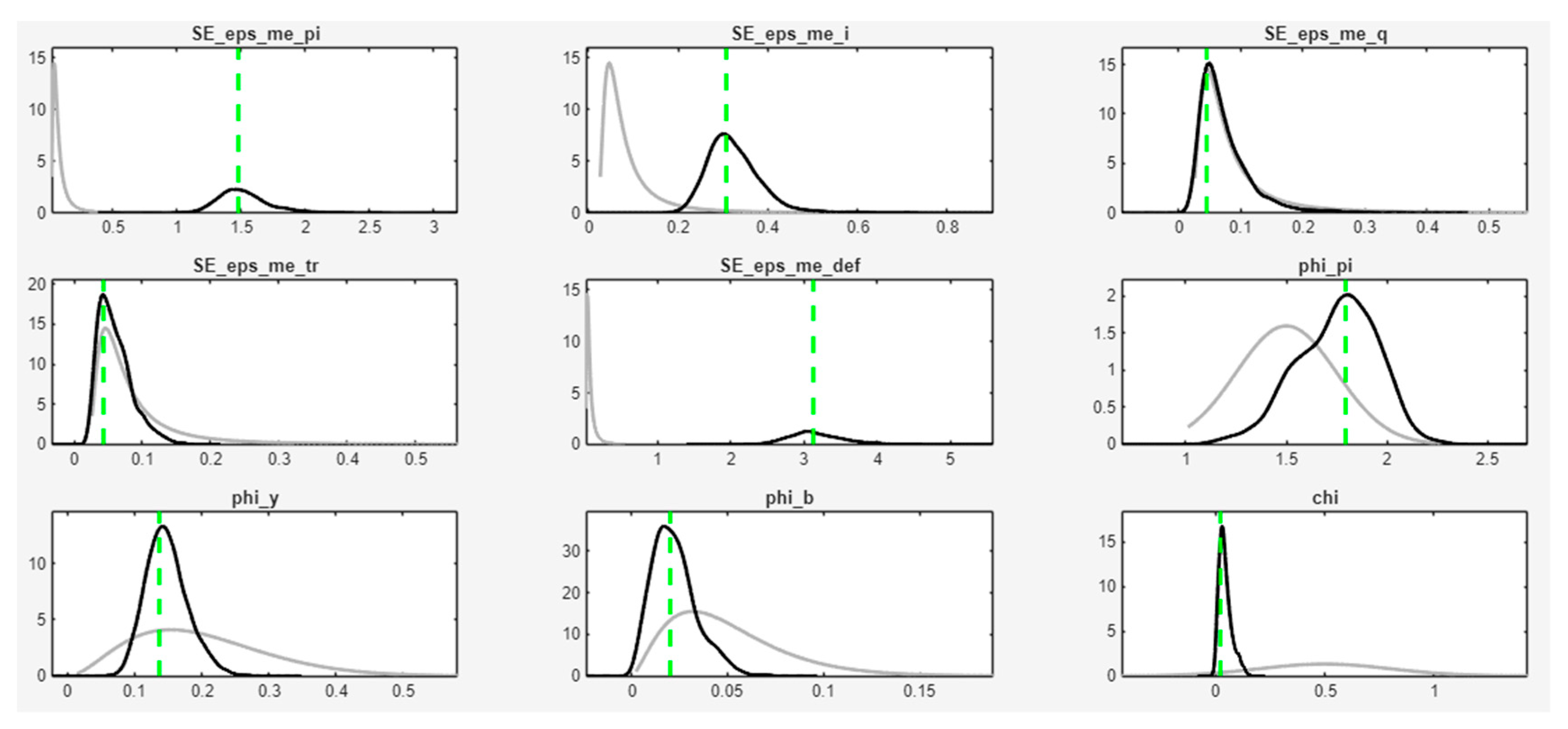
Table 2 presents the Bayesian estimation results of the DSGE model for Myanmar. We report posterior means and 90 percent Highest Posterior Density (HPD) intervals for the baseline specification. Overall, the data are highly informative, as posterior distributions are substantially tighter than their corresponding priors for most structural parameters.

3.3.1. Monetary Policy Behavior

The estimated Taylor rule indicates an active monetary policy stance, consistent with the Central Bank of Myanmar’s statutory emphasis on price stability. The posterior mean of the inflation response coefficient, ϕ π , is estimated at 1.75, with a 90 percent HPD interval of [1.43, 2.06], which lies entirely above unity. This result satisfies the Taylor principle and implies that the central bank systematically increased nominal interest rates by more than one-for-one in response to inflation deviations. In contrast, the estimated response to the output gap, ϕ y , is positive but modest (0.15), suggesting that monetary policy placed relatively limited weight on output stabilization. Taken together, these estimates indicate that monetary policy in Myanmar remained predominantly anti-inflationary, even amid substantial macroeconomic and political disruptions.

3.3.2. Fiscal Policy and Weak Discipline

The estimated government spending feedback coefficient on lagged debt, ϕ g , b , is small (0.022), with the lower bound of the HPD interval approaching zero. This suggests that fiscal authorities did not systematically reduce spending in response to rising debt levels. Complementarily, the tax revenue response to debt, ϕ τ , b , is estimated at −0.006 with a 90 percent HPD interval of [−0.026, 0.015] that includes zero, indicating that tax revenues also did not systematically adjust upward to stabilize rising debt. Taken together, both fiscal instruments exhibit negligible debt-stabilizing responses, reinforcing the characterization of fiscal policy as passive in the sense of Leeper (1991).

3.3.3. Political Instability and the Risk-Premium Channel

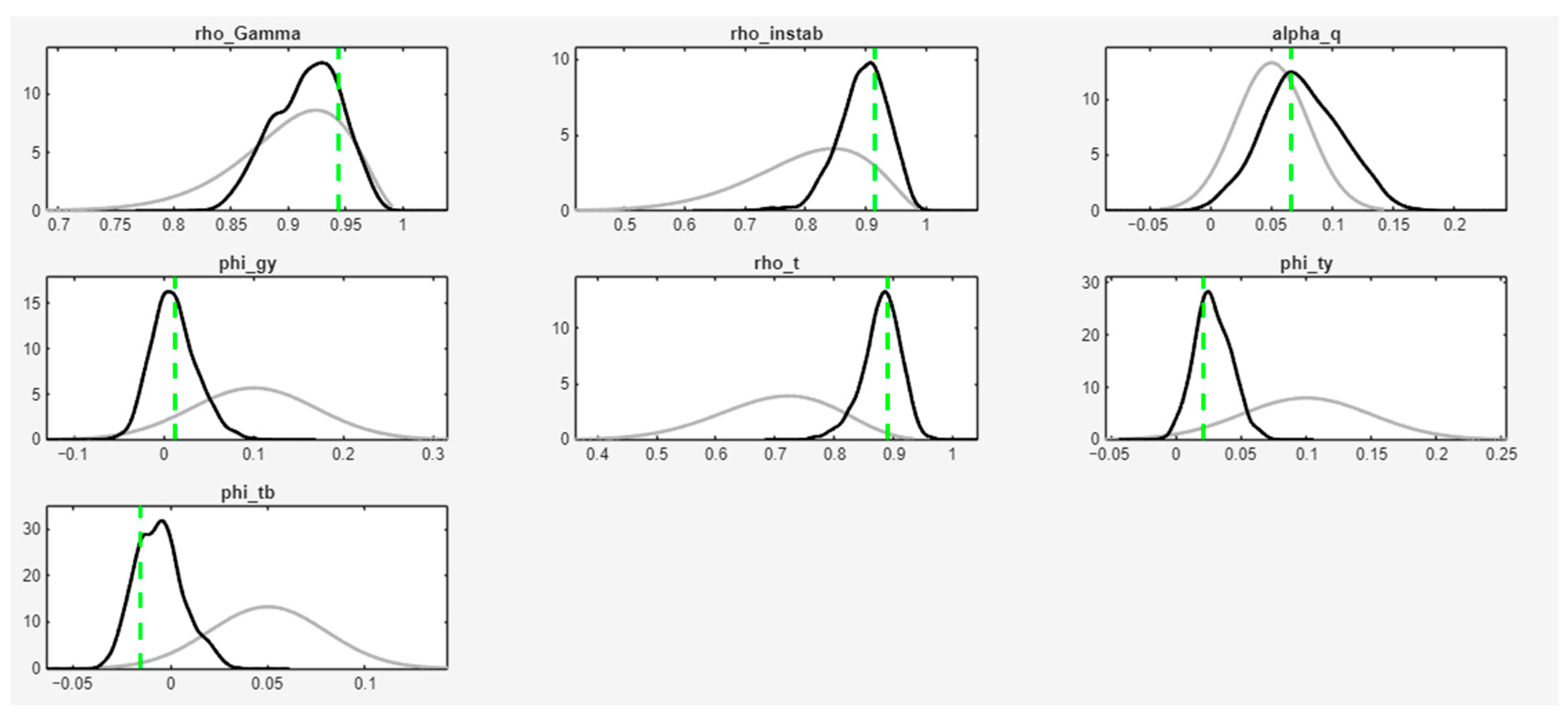
A central contribution of this paper is the identification of a political risk transmission mechanism. The sensitivity of the country risk premium to political instability, χ , is estimated to be positive and statistically significant, with a posterior mean of 0.046. Although this estimate is lower than the diffuse prior mean, the 90 percent HPD interval lies strictly in the positive domain, providing clear empirical evidence that political instability is associated with higher external financing costs. Political instability itself is highly persistent, with ρ instab estimated at approximately 0.90, while the persistence of the risk premium process is even higher, with ρ Γ 0.92 . These estimates imply that political shocks are not transitory events but instead generate long-lasting macroeconomic effects, primarily through sustained increases in perceived country risk that affect exchange rate and inflation dynamics. Visual plots of the prior and posterior distributions for all structural parameters are provided in Appendix A.

3.4. Shock Volatilities and Crisis Dynamics

The estimated volatility of the aggregate demand shock is exceptionally large, with σ y 11.3 , far exceeding typical business-cycle magnitudes. This result characterizes the post-2021 period as a severe demand-driven contraction, consistent with a sudden stop in private organization and investment driven by heightened uncertainty and confidence loss (Calvo, 1998). The Forecast Error Variance Decomposition (FEVD) further underscores the quantitative importance of the political risk channel. At the infinite horizon, risk premium shocks which are structurally linked to political instability account for approximately 33 percent of real exchange rate volatility and about 10 percent of inflation variability. These findings indicate that political instability constitutes a quantitatively important source of macroeconomic fluctuations in Myanmar, operating primarily through the exchange rate channel and contributing to imported inflation.

3.5. Impulse Response Analysis

To examine the dynamic transmission of macroeconomic shocks and assess the interaction between fiscal and monetary policy under political instability, we analyze impulse response functions (IRFs) generated from the estimated DSGE model. The IRFs trace the responses of key macroeconomic variables to one-standard-deviation structural shocks, holding all other innovations constant. Responses are reported over a 20-quarter horizon and are computed using posterior mean parameter estimates. Throughout this section, an increase in the real exchange rate denotes a real depreciation of the domestic currency. Tax revenue is denoted as τ ^ t in all figures, consistent with the notation adopted in Equation (5), where the Greek subscript τ distinguishes the tax variable from the time subscript t .

3.5.1. Political Instability Shock

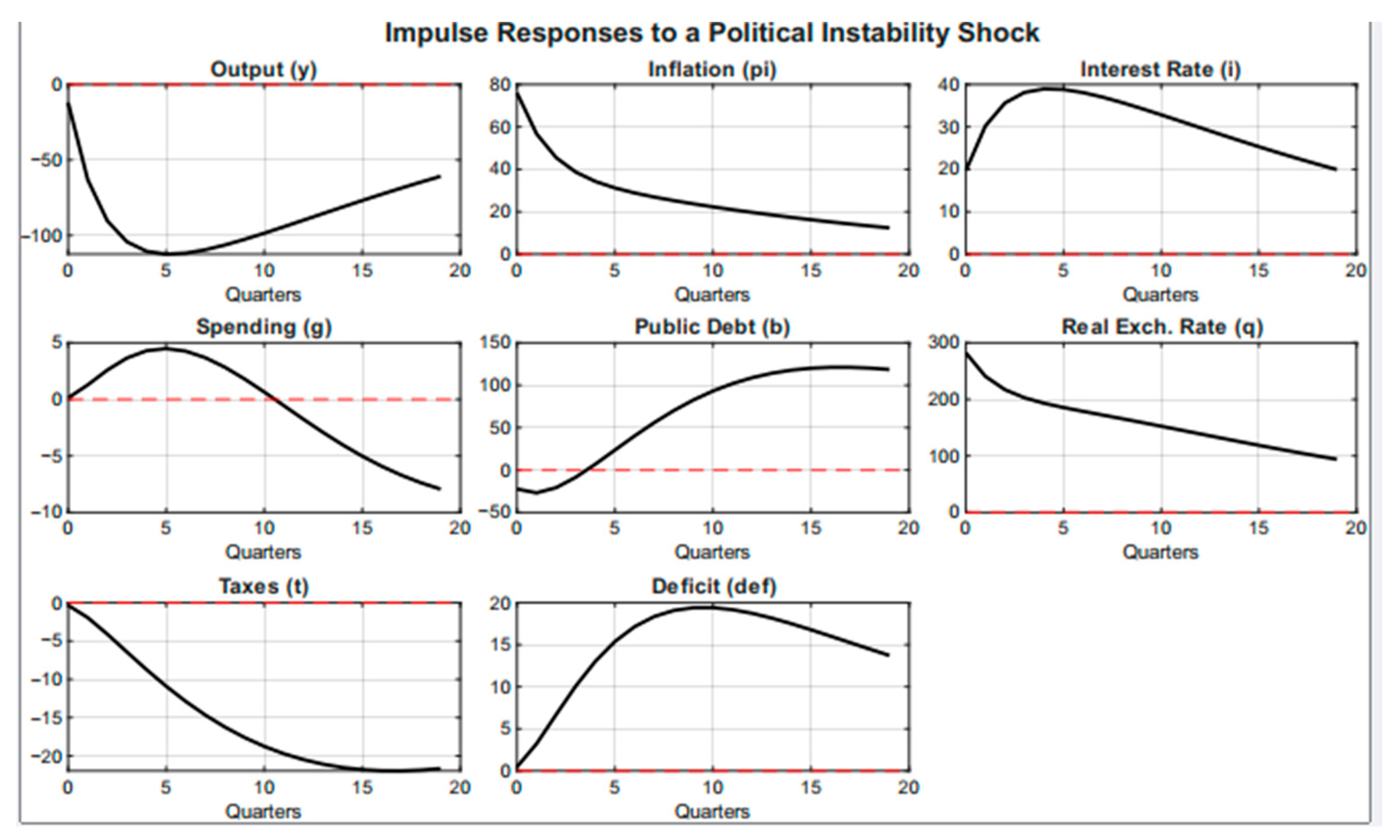
Figure 1 reports the responses to a positive shock to political instability. The shock generates a persistent increase in the country risk premium, reflecting heightened investor uncertainty and capital outflows. Because of Uncovered Interest Parity condition, the higher risk premium leads to an immediate and large depreciation of the real exchange rate. Through exchange rate pass-through, this depreciation leads to an increase in inflation. Output falls sharply after the shock because private consumption and investment decline under tighter external financing conditions and greater uncertainty. The output response is highly persistent, indicating that political instability has long-lasting negative effects on economic activity rather than temporary ones. Monetary policy responds by raising the policy interest rate in reaction to inflationary pressures. While this tightening contributes to inflation stabilization, it further reduces output and does not fully balance inflationary pressures caused by currency depreciation. Overall, the IRFs highlight that political instability leads to stagflation, characterized by simultaneously lower output and higher inflation.

3.5.2. Monetary Policy Shock

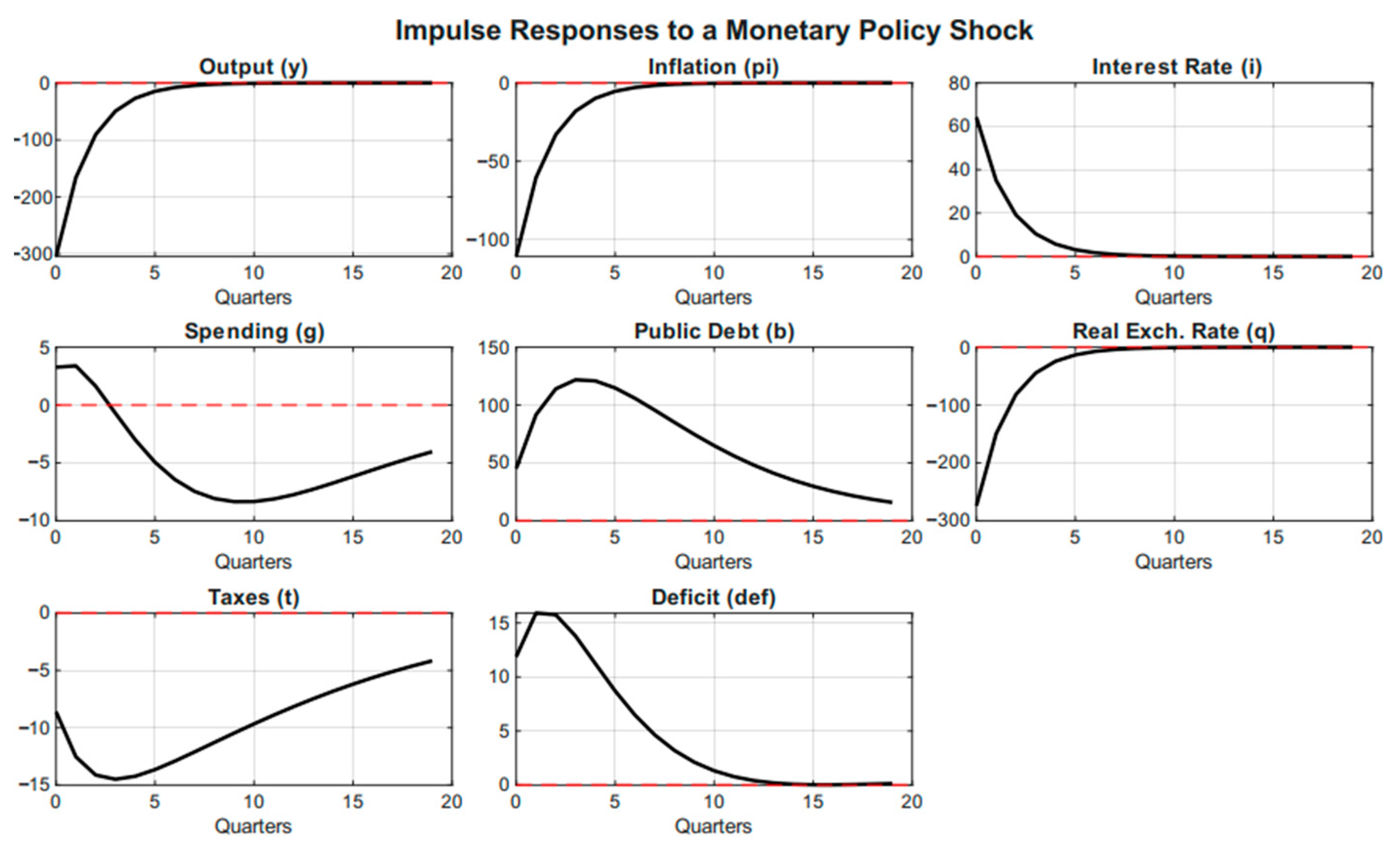
Figure 2 presents the responses to a contractionary monetary policy shock. An exogenous increase in the policy interest rate leads to an immediate decline in output and inflation, consistent with standard New Keynesian transmission mechanisms. A higher interest rate leads to a real exchange rate appreciation, which reduces external demand and deepens the decline in output. The fiscal consequences of monetary tightening are substantial. Through the debt-service channel ( η b ), higher interest rates raise debt-servicing costs and, at the same time, lower output reduces government tax revenues. As a result, public debt increases sharply in the short run. Given the weak fiscal response to debt (low ϕ g , b ), fiscal authorities do not sufficiently adjust spending or taxation to balance these pressures. Consequently, although monetary tightening lowers inflation in the short run, it leads to a temporary but significant rise in public debt. These dynamics highlight the high fiscal cost of monetary stabilization when fiscal discipline is weak.

3.5.3. Government Spending Shock

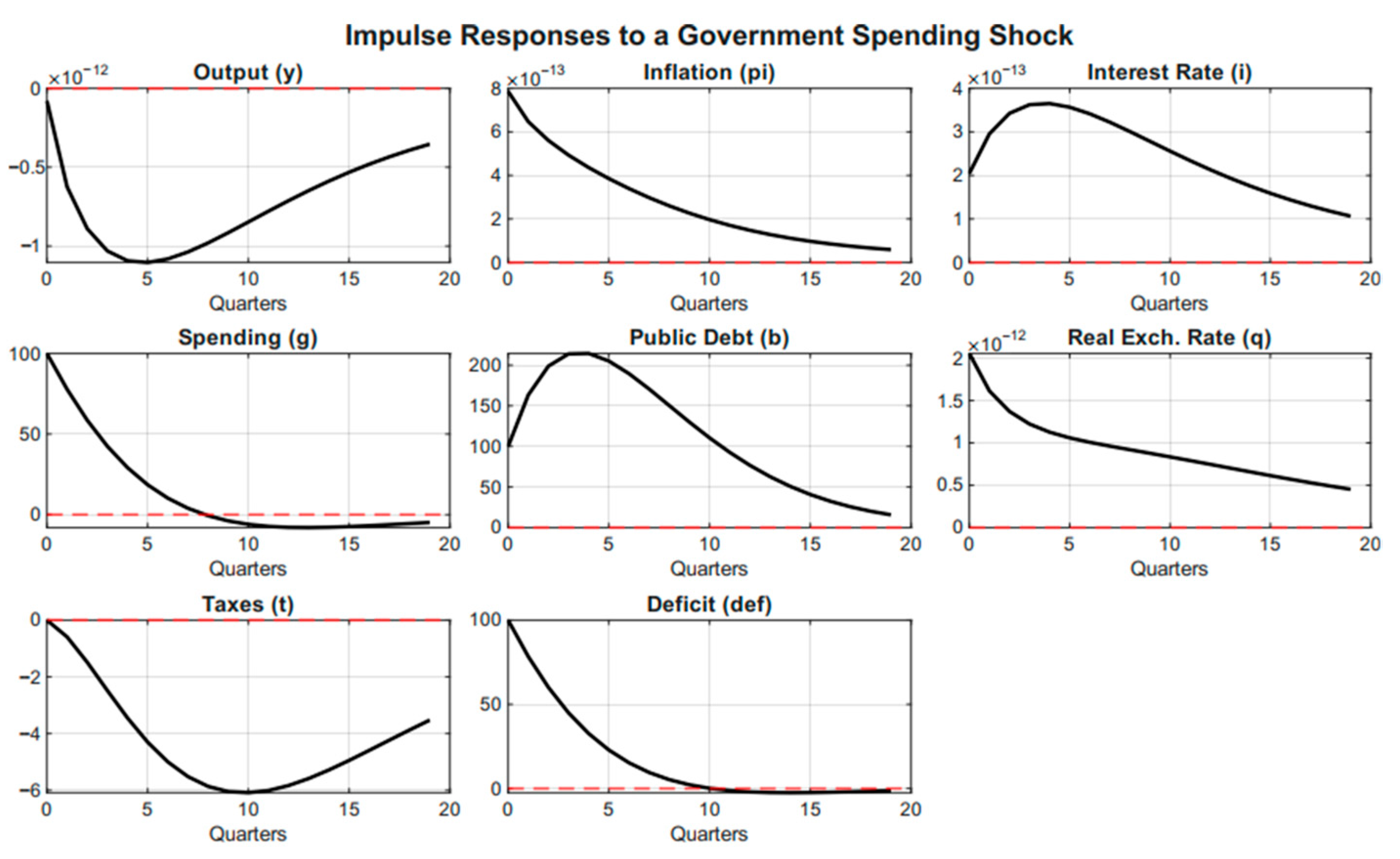
Figure 3 illustrates the effects of an expansionary government spending shock. The increase in public spending raises output in the short run through direct demand effects. However, this expansion is accompanied by a weaker fiscal balance and a sustained increase in public debt. In the absence of a strong debt-stabilizing fiscal response, the fiscal expansion places upward pressure on inflation and induces a real exchange rate depreciation. The central bank responds by tightening monetary policy, which crowds out private investment and partially balances the initial gains in output. Importantly, the interaction between higher interest rates and weak fiscal feedback amplifies debt accumulation dynamics over time. These responses highlight the destabilizing effects of fiscal expansion when fiscal credibility is low and public debt is weakly anchored.

3.5.4. Policy Interaction and Regime Implications

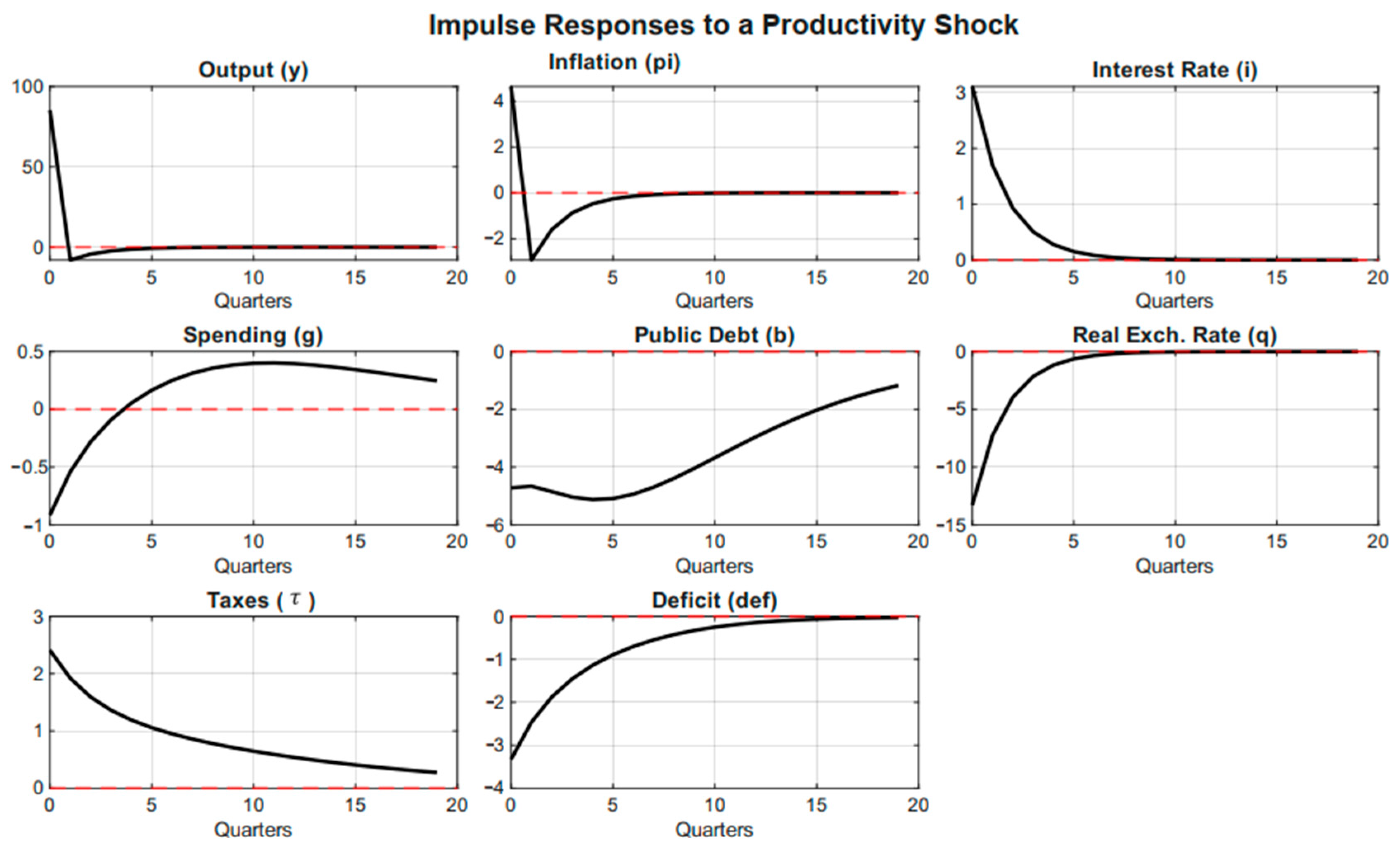
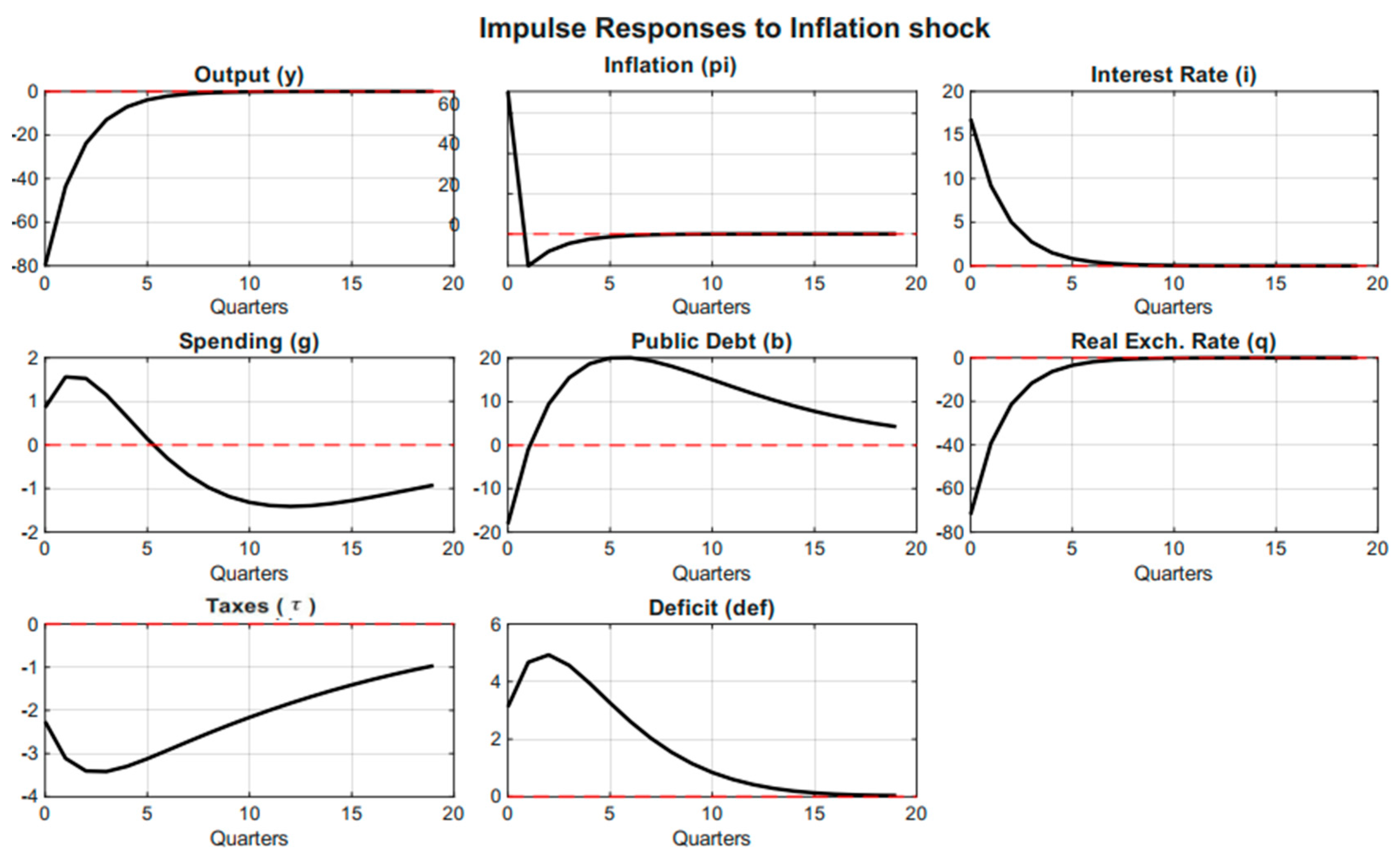
Monetary policy behaves actively in response to inflationary pressures, consistent with the Taylor principle, while fiscal policy remains largely passive with respect to debt stabilization. This asymmetry undermines the overall coherence of the macroeconomic policy framework. In particular, the interaction between political instability and weak fiscal discipline generates a reinforcing feedback loop. Political instability increases the risk premium and inflation which lead to monetary tightening, while higher interest rates further worsen fiscal imbalances by raising debt-servicing costs. Within the estimated model, these dynamics explain why post-2021 macroeconomic outcomes in Myanmar are driven by tensions between strict monetary policy and weak fiscal capacity, which are amplified by persistent political instability. While this section focuses on the primary shocks of interest, additional impulse response functions for productivity, inflation, public debt, country risk premium, and tax shocks are provided in Appendix A (Figure A4, Figure A5, Figure A6, Figure A7 and Figure A8).

3.6. Robustness Analysis

3.6.1. Numerical Stability and MCMC Convergence

We first evaluate the numerical stability of the posterior estimates by re-estimating the baseline model using a substantially longer Markov Chain Monte Carlo (MCMC) sequence. While the baseline results are obtained using 20,000 Metropolis–Hastings replications, this robustness exercise extends the chain length to 50,000 replications. The resulting posterior estimates remain highly stable. In particular, the sensitivity of the country risk premium to political instability, χ , is estimated at 0.047, compared to 0.046 in the baseline specification. Likewise, the monetary policy response to inflation, ϕ π , remains firmly above unity at approximately 1.87, confirming an active monetary policy stance. Standard convergence diagnostics (Brooks & Gelman, 1998) indicate well-behaved chains and stable posterior moments, providing confidence that the baseline estimation adequately approximates the related distribution.

3.6.2. Structural Robustness: Acyclical Fiscal Policy

We next examine whether the baseline results depend on the assumption that government spending responds to cyclical economic conditions. In the baseline specification, government spending reacts to both lagged public debt and the output gap. However, in many developing and conflict-affected economies, fiscal policy may lack the institutional capacity to conduct discretionary countercyclical stabilization (Frankel et al., 2013). To capture this possibility, we impose a cyclical fiscal spending rule by restricting the output gap feedback coefficient to zero: ϕ g , y = 0 . Under this restricted specification, government spending responds only to debt dynamics and exogenous fiscal shocks. The estimation results confirm that the main conclusions are unaffected. The fiscal response to public debt, ϕ g , b , remains statistically negligible (approximately 0.022), reinforcing the characterization of fiscal policy as passive. At the same time, the political risk transmission parameter, χ , remains positive and statistically significant at 0.046, indicating that political instability continues to raise the country risk premium even in the absence of countercyclical fiscal spending.

3.6.3. Sensitivity to Alternative Priors

To address concerns regarding the influence of baseline prior selections on a short data sample, we conducted a sensitivity analysis utilizing alternative prior distributions. Specifically, we tested the robustness of the central political risk transmission parameter χ by substituting the baseline Normal prior with a diffuse Uniform distribution, thereby removing any advanced-economy distributional assumptions. Under this uninformative prior, the posterior mean for χ remains strictly positive and quantitatively stable (approximately 0.045), confirming that the empirical data rather than the selected prior drives the conclusion that political instability significantly raises the country risk premium. Similar stability is observed when widening the prior variances for the monetary and fiscal feedback rules, confirming the external validity of the estimated policy conflict regime.
Table 3 reports posterior estimates for key structural parameters across the baseline model and two robustness specifications. The inflation response coefficient Φ π remains well above unity in all cases, confirming that the central bank maintains an active anti-inflationary stance regardless of the fiscal specification. Conversely, fiscal policy consistently exhibits a negligible response to public debt ϕ b 0.02 , a finding that is robust across all scenarios. This persistence of weak fiscal feedback, combined with active monetary policy, corroborates the existence of a policy conflict regime rather than standard fiscal dominance (Leeper, 1991). Crucially, the transmission of political instability to the country risk premium χ remains positive and stable, confirming that political turmoil acts as a structural and exogenous driver of external financial stress. The high persistence of both political instability and the risk premium implies that these shocks generate prolonged macro-financial cycles. Overall, the robustness analysis confirms that the twin drivers of Myanmar’s macroeconomic instability, weak fiscal discipline and politically driven risk premia, are structural features of the economy rather than artifacts of specific modeling assumptions or numerical settings.

3.7. Forecast Error Variance Decomposition

To quantify the relative importance of structural shocks in driving macroeconomic fluctuations, we conduct a forecast error variance decomposition (FEVD) at the infinite horizon. This analysis provides a systematic assessment of the dominant sources of variability in output, inflation, and the real exchange rate in Myanmar. The results reported in Table 4 indicate that aggregate demand shocks overwhelmingly dominate real economic activity, accounting for approximately 99% of output variance across all model specifications. This finding reinforces the interpretation of the post-2021 contraction as a severe demand-driven collapse consistent with a sudden stop in consumption and investment rather than a supply-side productivity slowdown (Calvo, 1998). In contrast, inflation and exchange rate dynamics are strongly shaped by external financial conditions and political instability. The combined political risk channel, defined as shocks to the country risk premium ( ε Γ , t ) and to political instability ( ε instab , t ), accounts for approximately 18% of inflation variability. This highlights the importance of politically driven external pressures in shaping domestic price dynamics.
Most strikingly, the political risk channel emerges as the dominant driver of real exchange rate fluctuations. Together, risk premium and political instability shocks explain over 52% of real exchange rate variance in the baseline specification, with contributions of 33.1% and 19.0%, respectively. This result underscores the central role of political turmoil in driving currency depreciation, which subsequently feeds into inflation through the exchange rate pass-through mechanism. Monetary policy shocks contribute only modestly to inflation variability (7.3%) and to interest rate fluctuations (5.3%), while fiscal shocks primarily affect government spending and public debt dynamics, with limited spillovers to aggregate output or inflation. These patterns are consistent with a regime of policy conflict (Leeper, 1991), in which the effectiveness of monetary policy is constrained by weak fiscal discipline and the predominance of politically driven external shocks.
Importantly, the FEVD results are highly robust across alternative fiscal policy specifications. The dominance of demand shocks in explaining output volatility and the critical role of the political risk channel in driving exchange rate fluctuations remain stable across models. Taken together, these findings provide further support for the paper’s central conclusion that political instability constitutes a distinct and quantitatively significant source of macroeconomic volatility in Myanmar.

4. Conclusions and Implications

This paper examines the interaction between fiscal and monetary policy in Myanmar within a small open-economy New Keynesian DSGE framework, explicitly incorporating political instability as a structural driver of macroeconomic dynamics. Using Bayesian estimation on quarterly data from 2013 to 2022, the analysis provides quantitative evidence on the mechanisms underlying Myanmar’s post-2021 stagflation episode. Three central findings emerge.
First, the post-transition economic collapse is driven by aggregate demand contraction rather than a conventional supply-side downturn. Forecast error variance decomposition shows that aggregate demand shocks account for approximately 99 percent of output volatility, consistent with a sudden stop in consumption and investment driven by uncertainty and a collapse in confidence rather than by productivity or supply-side disruptions. Second, the results identify a regime of policy conflict rather than standard fiscal weakness. While the Central Bank of Myanmar is estimated to have maintained an active anti-inflationary stance satisfying the Taylor principle, the fiscal authority does not systematically respond to rising public debt ( ϕ g , b 0.02 ). This asymmetry generates a structural inconsistency: monetary tightening aimed at stabilizing inflation raises debt-servicing costs through the debt-service channel, worsening fiscal stress and undermining the overall coherence of macroeconomic stabilization. Third, political instability plays a quantitatively dominant role through the external sector. Shocks to political instability and the country risk premium together explain more than 52 percent of real exchange rate volatility, confirming that political turmoil is not merely a background condition but a structural driver of currency depreciation and imported inflation, operating independently of standard macroeconomic fundamentals.
The core policy conclusion is clear: without fiscal discipline and political stabilization, monetary policy alone cannot deliver macroeconomic stability in fragile and conflict-affected economies. Future research could extend this framework to incorporate regime-switching behavior, explicit financial sector channels, non-linear crisis dynamics, and the role of informal markets. It is important, however, to acknowledge the specific limitations of the present study explicitly, as they define both the boundary conditions of our findings and productive avenues for future research.

4.1. On the Representative-Agent Framework

Due to the severe lack of high-frequency household microdata in Myanmar, this paper relies on a representative-agent New Keynesian (RANK) framework. The recent literature has increasingly moved toward heterogeneous-agent New Keynesian (HANK) models, which incorporate household heterogeneity, liquidity constraints, and distributional channels of policy transmission. Seminal contributions by Kaplan et al. (2018) demonstrate that monetary policy operates primarily through indirect general equilibrium income effects rather than the direct intertemporal substitution channel emphasized in RANK models, while Auclert (2019) formalizes redistribution channels through which interest rate changes affect aggregate consumption via heterogeneous balance sheet exposures. We are fully aware of these developments. However, HANK models require granular household-level microdata on wealth distributions and portfolio composition to discipline their key structural parameters—data that are effectively unavailable for Myanmar. Furthermore, as Acharya and Dogra (2020) note, the gains from HANK over RANK are most pronounced in economies with deep and accessible financial markets, precisely the conditions absent in Myanmar’s bank-dependent, cash-based economy. Future research could productively incorporate HANK structures to evaluate distributional consequences of the identified policy conflict regime once granular household data become available.

4.2. On the Informal Economy, External Sector Dynamics, and Financial Repression

A further important limitation concerns the paper’s abstraction from three structural features that are quantitatively significant in Myanmar’s economy: the informal sector, dual exchange rate dynamics, and financial repression. Each represents a channel through which the estimated policy transmission mechanisms may differ from those operating in practice.
Regarding the informal economy, Myanmar has one of the largest informal sectors in Southeast Asia, with informal economic activity accounting for a substantial share of total output, employment, and household income. In fragile and conflict-affected states, the informal sector constitutes an active parallel economy with its own price-setting dynamics, credit channels, and responses to fiscal and monetary policy (Loayza, 1996; Elgin & Oztunali, 2012). The standard New Keynesian transmission mechanisms—which operate through formal credit markets, interest-sensitive investment, and observable price indices—therefore capture only a partial picture of aggregate dynamics. In particular, the CPI-based inflation measure used in our estimation reflects primarily formal sector prices, potentially understating the inflationary impact of exchange rate depreciation on households whose shopping basket is disproportionately sourced from informal markets. Future research incorporating a dual-sector framework with explicit informal economy dynamics, along the lines of Batini et al. (2010), would enrich the characterization of monetary policy transmission in Myanmar’s fragile institutional environment.
Regarding dual exchange rate dynamics, Myanmar operated a managed official exchange rate alongside a widely used parallel market rate throughout the sample period, with the spread between the two rates widening dramatically following the 2021 political transition. The real exchange rate series used in our estimation is constructed from the official rate, which may not accurately reflect the effective exchange rate faced by private agents conducting transactions through informal currency markets. This measurement discrepancy has direct implications for the estimated exchange rate pass-through coefficient α q and the UIP-based risk premium channel in Equation (7), both identified partly through observed exchange rate movements. To the extent that the official rate was administratively managed and partially disconnected from market conditions during the post-2021 period, our estimates of the political risk transmission channel may understate the true magnitude of pass-through to domestic prices. Incorporating a dual exchange rate structure would provide a more accurate characterization of external sector dynamics and represents a productive avenue for future research once sufficiently long parallel market rate series become available.
Regarding financial repression, Myanmar’s banking sector is characterized by directed lending, interest rate ceilings, and significant state ownership of financial institutions, which collectively suppress the normal market-based transmission of monetary policy through the credit channel. In an environment of financial repression, central bank interest rate changes may have limited traction over private sector borrowing costs, as state-owned banks are not fully responsive to policy rate signals and informal lenders operate entirely outside the regulatory perimeter. This implies that the estimated monetary policy transmission coefficients, which assume a standard interest rate channel operating through competitive financial markets, may overstate the effective reach of monetary tightening in practice. Acknowledging these constraints is consistent with the broader literature on monetary policy effectiveness in financially repressed emerging economies (McKinnon, 1973; Shaw, 1973; Giovannini & De Melo, 1993) and reinforces our central conclusion that monetary tightening alone is insufficient to restore macroeconomic stability without accompanying structural reforms to the financial system and fiscal framework.
Taken together, these limitations—informal sector dynamics, dual exchange rate markets, and financial repression—suggest that the quantitative estimates presented in this paper should be interpreted as characterizing the formal economy’s response to the identified shocks, rather than capturing the full general equilibrium effects across all segments of Myanmar’s complex economic structure. Importantly, these considerations do not undermine the paper’s central findings regarding the policy conflict regime and the political risk transmission channel, which are identified through structural variation in observable macroeconomic aggregates and remain robust across all alternative specifications. Rather, they define a clear and productive agenda for future structural empirical work on fragile and conflict-affected frontier economies.


Author Contributions

Conceptualization, A.K.P. and C.S.; methodology, A.K.P. and C.S.; software, A.K.P.; validation, A.K.P., C.S. and N.P.; formal analysis, A.K.P.; investigation, A.K.P.; resources, A.K.P.; data curation, A.K.P.; writing—original draft preparation, A.K.P.; writing—review and editing, A.K.P. and C.S.; visualization, A.K.P.; supervision, C.S. and N.P.; project administration, C.S. and N.P.; funding acquisition, C.S. and N.P. All authors have read and agreed to the published version of the manuscript.

Funding

This research received no external funding.

Institutional Review Board Statement

Not applicable.

Informed Consent Statement

Not applicable.

Data Availability Statement

The macroeconomic data supporting this study are derived from public domain resources, including the World Bank, the IMF, the Central Bank of Myanmar, and the Ministry of Planning and Finance. The political instability index data and supplementary macroeconomic series were obtained from CEIC Data. These proprietary datasets are subject to third-party restrictions and are not publicly available. The data and Dynare replication files that support the findings of this study are available from the corresponding author upon reasonable request, subject to permission from CEIC.

Acknowledgments

The author wishes to thank senior candidate Htwe Ko for invaluable support when it comes to submitting the journal, formatting and research and feedback throughout the development of this research. The author also gratefully acknowledges the helpful comments and suggestions from the participants of the Spring International 5th Conference, which greatly improved this manuscript. Finally, the author extends thanks to the Faculty of Economics, Chiang Mai University for their institutional support.

Conflicts of Interest

The authors declare no conflicts of interest.

Appendix A

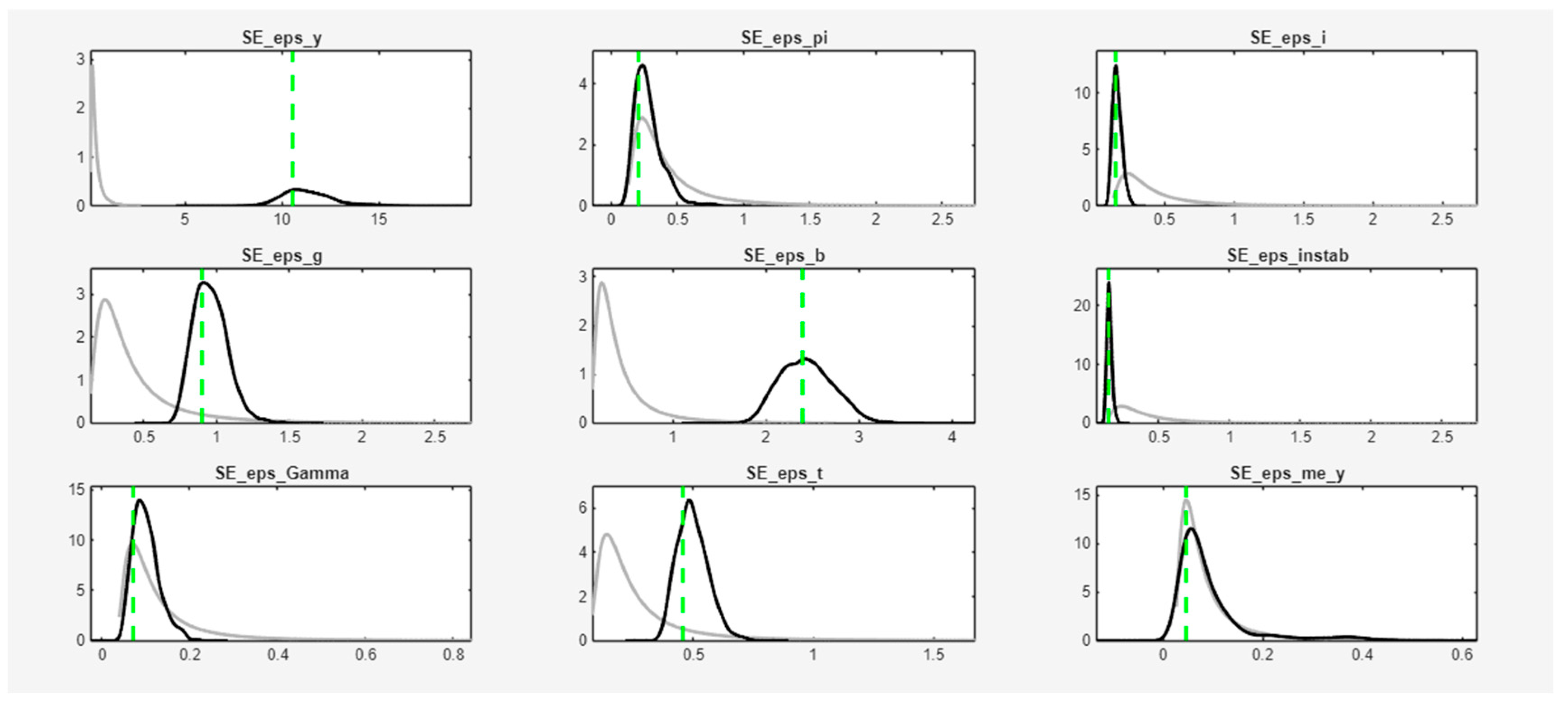
Figure A1. Prior and posterior distributions of structural parameters. Note: The gray solid line represents the prior distribution, the black solid line represents the posterior distribution, and the green dashed line indicates the posterior mode obtained from the numerical optimization.
Economies 14 00157 g0a1
Figure A2. Prior and posterior distributions of structural parameters. Note: The gray solid line represents the prior distribution, the black solid line represents the posterior distribution, and the green dashed line indicates the posterior mode obtained from the numerical optimization.
Economies 14 00157 g0a2
Figure A3. Prior and posterior distributions of structural parameters. Note: The gray solid line represents the prior distribution, the black solid line represents the posterior distribution, and the green dashed line indicates the posterior mode obtained from the numerical optimization.
Economies 14 00157 g0a3
Figure A4. Impulse responses to a productivity shock. Note: Impulse responses of key macroeconomic variables to a one-standard-deviation positive productivity shock. The horizontal axis represents quarters following the shock, and the vertical axis shows the percentage deviation from the steady state. Solid lines denote the posterior mean estimates.
Economies 14 00157 g0a4
Figure A5. Impulse responses to an inflation shock. Note: Impulse responses of key macroeconomic variables to a one-standard-deviation positive inflation (cost-push) shock. The horizontal axis represents quarters following the shock, and the vertical axis shows the percentage deviation from the steady state. Solid lines denote the posterior mean estimates.
Economies 14 00157 g0a5
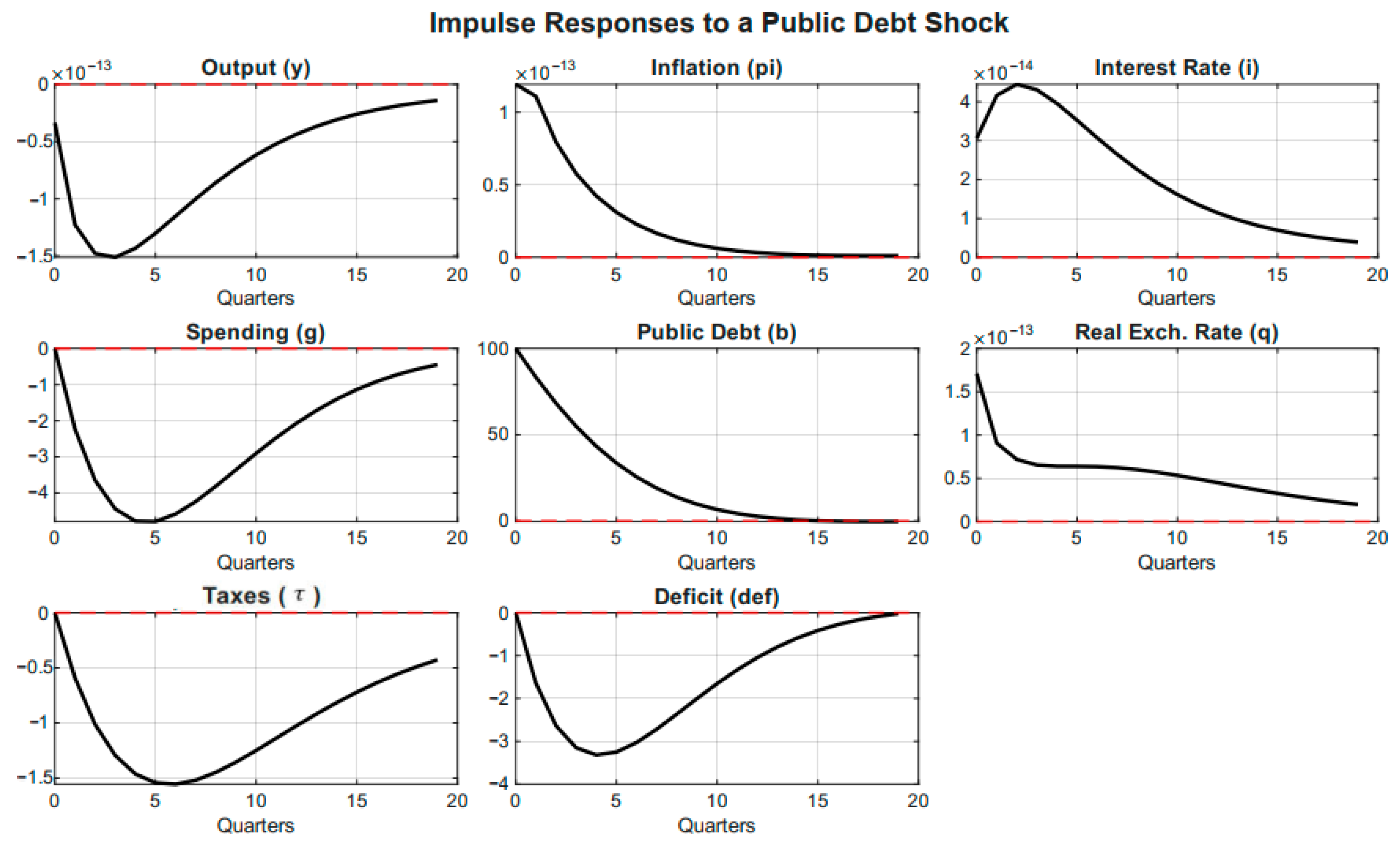
Figure A6. Impulse responses to a public debt shock. Note: Impulse responses of key macroeconomic variables to a one-standard-deviation positive public debt shock. The horizontal axis represents quarters following the shock, and the vertical axis shows the percentage deviation from the steady state. Solid lines denote the posterior mean estimates.
Economies 14 00157 g0a6
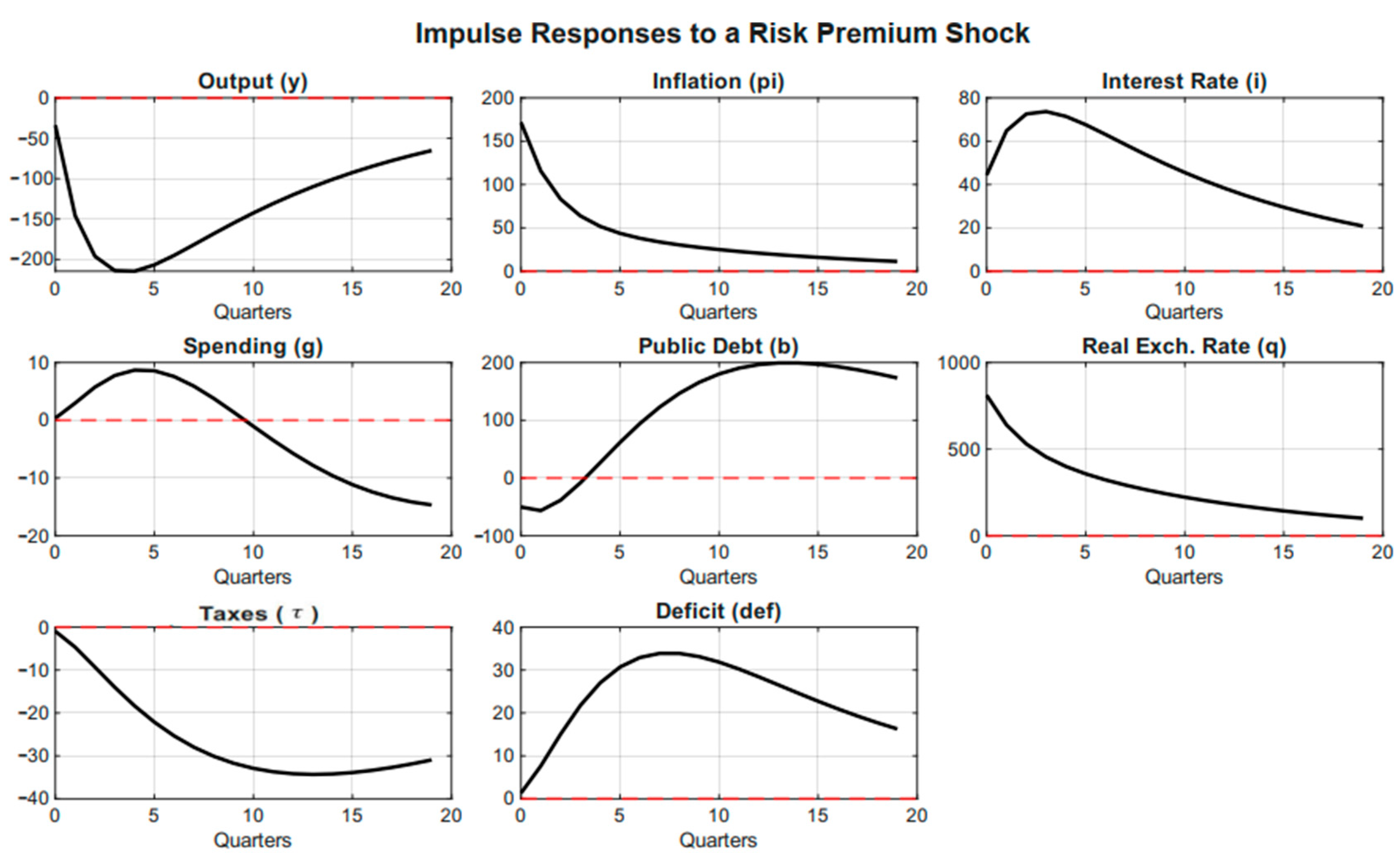
Figure A7. Impulse responses to a country risk premium shock. Note: Impulse responses of key macroeconomic variables to a one-standard-deviation positive country risk premium shock. The horizontal axis represents quarters following the shock, and the vertical axis shows the percentage deviation from the steady state. Solid lines denote the posterior mean estimates.
Economies 14 00157 g0a7
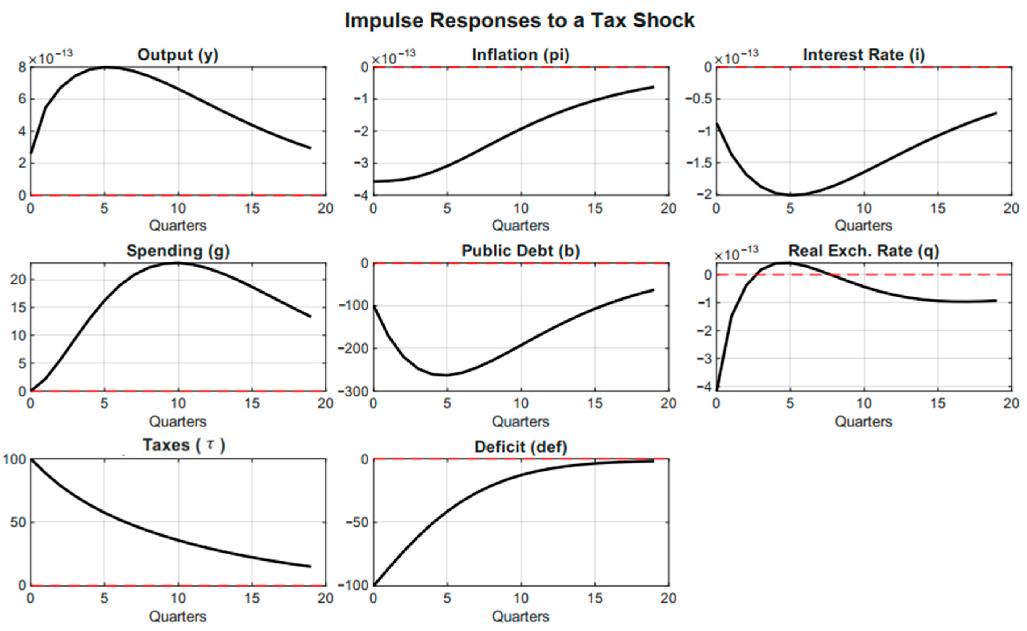
Figure A8. Impulse responses to a tax policy shock. Note: Impulse responses of key macroeconomic variables to a one-standard-deviation positive tax shock. The horizontal axis represents quarters following the shock, and the vertical axis shows the percentage deviation from the steady state. Solid lines denote the posterior mean estimates.
Economies 14 00157 g0a8

Appendix B. Theoretical Model Derivations

This appendix provides the full log-linearized derivations for all structural equations of the small open-economy New Keynesian (SOE-NK) model estimated in this paper, building upon the frameworks of Galí and Monacelli (2005) and Justiniano and Preston (2010). Hats (^) denote log-deviations from the deterministic steady state. All derivations proceed by taking a first-order Taylor expansion around a zero-inflation, deterministic steady state in which the real interest rate equals the inverse of the discount factor, r = 1 β 1 .

Appendix B.1. The Household’s Consumption Euler Equation

The representative household maximizes expected lifetime utility subject to the intertemporal budget constraint. The first-order condition with respect to nominal bond holdings yields the standard nonlinear Euler equation:
1 = β E t C t + 1 C t σ 1 + i t Π t + 1
Taking the natural logarithm of both sides:
0 = l o g β + E t σ ( c t + 1 c t ) + l o g ( 1 + i t ) l o g Π t + 1
Linearizing around the steady state where Π = 1 , i = ρ = 1 β 1 , and using the approximations l o g ( 1 + i t ) i t and l o g Π t + 1 π t + 1 :
0 = E t σ ( c ^ t + 1 c ^ t ) + i ^ t π ^ t + 1
Rearranging for current consumption yields, the log-linearized consumption Euler equation:
c ^ t = E t c ^ t + 1 1 σ ( i ^ t E t π ^ t + 1 ) + ε c , t
where σ > 0 is the inverse of the intertemporal elasticity of substitution and ε c , t is an exogenous preference shock capturing structural shifts in desired intertemporal consumption growth. Current consumption depends on expected future consumption minus the ex ante real interest rate gap, scaled by the intertemporal elasticity 1 σ .

Appendix B.2. The Open-Economy IS Curve

In a small open economy, domestic output Y t must satisfy the goods market clearing condition, equating production to domestic absorption and net exports. Following Galí and Monacelli (2005), domestic consumption deviates from domestic output proportionally to the real exchange rate q t , reflecting substitution between domestic and foreign goods:
c ^ t = y ^ t ψ q ^ t
where ψ > 0 captures the degree of trade openness and sensitivity of domestic demand to external competitiveness. Substituting this open-economy consumption–output relationship into the household Euler equation derived in Appendix B.1:
y ^ t ψ q ^ t = E t [ y ^ t + 1 ψ q ^ t + 1 ] 1 σ ( i ^ t E t π ^ t + 1 ) + ε y , t
Rearranging and assuming that real exchange rate expectations are sufficiently persistent so that E t q ^ t + 1 enters the current-period IS relationship through the contemporaneous real exchange rate term yields the open-economy IS curve estimated in Equation (1):
y ^ t = E t y ^ t + 1 1 σ ( i ^ t E t π ^ t + 1 ) + ψ q ^ t + ε y , t
where y ^ t is the output gap, i ^ t the nominal interest rate deviation from the steady state, E t π ^ t + 1 expected inflation, q ^ t the real exchange rate, and ε y , t an exogenous aggregate demand shock. The real exchange rate channel ψ q ^ t captures the expenditure-switching effect: a real depreciation raises the relative price of foreign goods, stimulating domestic demand.

Appendix B.3. The Open-Economy New Keynesian Phillips Curve

The supply side consists of a continuum of monopolistically competitive firms indexed by j [ 0 , 1 ] , each producing with technology Y t ( j ) = A t N t ( j ) . Prices are set on a staggered basis à la Calvo (1983). In each period, a fraction 1 θ of firms optimally reset their prices while the remaining fraction θ keep prices unchanged. The optimal reset price P t * solves:
k = 0 ( β θ ) k E t Y t + k ( j ) P t * ϵ ϵ 1 Ψ t + k = 0
where ϵ is the elasticity of substitution across varieties and Ψ t + k is the nominal marginal cost. Log-linearizing the optimal price-setting condition and aggregating across firms yields the domestic inflation equation:
π ^ H , t = β E t π ^ H , t + 1 + λ m c ^ t
where λ = 1 θ ) ( 1 β θ θ is the slope of the Phillips curve and m c ^ t denotes real marginal costs expressed as log-deviations from the steady state. In an open economy, real marginal costs depend on the domestic output gap and the real exchange rate, reflecting both domestic factor costs and the price of imported intermediate inputs. Furthermore, overall CPI inflation π ^ t is a weighted average of domestic inflation π ^ H , t and imported inflation, which is driven by movements in the real exchange rate. Substituting the expression for marginal costs in terms of the output gap and the real exchange rate, and mapping domestic inflation to CPI inflation through the import price channel, yields the open-economy NKPC estimated in Equation (2):
π ^ t = β E t π ^ t + 1 + κ y ^ t + α q q ^ t + ε π , t
where κ > 0 is the composite slope parameter measuring the sensitivity of inflation to domestic economic activity, α q > 0 captures exchange rate pass-through to CPI inflation, and ε π , t is an exogenous cost-push shock capturing non-demand supply disturbances such as commodity price movements or markup shocks.

Appendix B.4. The Monetary Policy Rule

The monetary policy rule in Equation (3) is specified as an empirical interest rate feedback rule of the inertial Taylor type, following the extensive literature on estimated monetary policy rules (Taylor, 1993; Clarida et al., 1999; Woodford, 2003). Rather than being derived from an explicit central bank optimization problem, this rule represents a reduced-form characterization of systematic monetary policy behavior. In log-linear form:
i ^ t = ρ i i ^ t 1 + ( 1 ρ i ) ( ϕ π π ^ t + ϕ y y ^ t ) + ε i , t
The smoothing parameter ρ i [ 0 , 1 captures the empirically well-documented tendency of central banks to adjust policy rates gradually, avoiding large discrete changes that could destabilize financial markets. The parameters ϕ π and ϕ y govern the systematic response to inflation deviations and the output gap, respectively. The Taylor principle requires ϕ π > 1 , ensuring that the nominal interest rate rises by more than one-for-one with inflation, thereby raising the real interest rate and providing a stabilizing force against inflationary pressures. This condition is necessary for nominal determinacy under active monetary policy (Leeper, 1991; Woodford, 2003). The Bayesian posterior estimate of ϕ π = 1.75 with a 90 percent HPD interval of 1.43 2.06 , lying entirely above unity, confirms that the Central Bank of Myanmar maintained an active anti-inflationary monetary policy stance throughout the sample period. The term ε i , t captures exogenous monetary policy shocks reflecting discretionary deviations from the systematic rule.

Appendix B.5. The Uncovered Interest Parity Condition

Under imperfect international capital mobility, the relationship between domestic and foreign assets is governed by a risk-adjusted no-arbitrage condition. Let E t denote the nominal exchange rate (domestic currency per unit of foreign currency). The nominal UIP condition is:
1 + i t = ( 1 + i t * ) E t E t + 1 E t Φ t
where i t * is the foreign interest rate and Φ t is the gross country risk premium. We define the real exchange rate as Q t = E t P t * P t , so that an increase in Q t denotes a real depreciation. Taking logs and linearizing around the steady state where Φ = 1 :
i ^ t = i ^ t * + E t q ^ t + 1 q ^ t + E t π ^ t + 1 E t π ^ t + 1 * + Γ t
where Γ t = l o g Φ t denotes the log-deviation of the country risk premium from its steady-state value. Assuming a constant foreign price level such that E t π ^ t + 1 * = 0 and rearranging for the current real exchange rate q ^ t yields the log-linearized real UIP condition estimated in Equation (7):
q ^ t = E t q ^ t + 1 ( i ^ t E t π ^ t + 1 i ^ t * ) + Γ t
This expression states that the current real exchange rate equals its expected future value minus the real interest rate differential between domestic and foreign assets, adjusted for the country risk premium. An increase in Γ t , reflecting higher perceived country risk, induces an immediate real depreciation, which is the key transmission channel through which political instability affects the exchange rate and subsequently inflation.

Appendix B.6. Fiscal Policy Rules

The government spending and tax revenue rules are specified as empirical fiscal reaction functions following Leeper (1991) and Blanchard and Perotti (2002). These rules represent reduced-form characterizations of fiscal behavior that are standard in the empirical DSGE literature for emerging economies, capturing the systematic response of fiscal instruments to macroeconomic conditions.
Government spending responds inertially to its own lagged value, the current output gap, and the lagged public debt level:
g ^ t = ρ g g ^ t 1 ϕ g , y y ^ t ϕ g , b b ^ t 1 + ε g , t
The negative sign on ϕ g , y > 0 implies countercyclical spending behavior—government spending falls when output rises above potential—while the negative sign on ϕ g , b > 0 implies fiscal consolidation in response to rising debt. The persistence parameter ρ g ( 0 , 1 ) captures budgetary rigidities and implementation lags that prevent immediate adjustment of spending plans.
Tax revenues follow an analogous feedback structure:
τ ^ t = ρ τ τ ^ t 1 + ϕ τ , y y ^ t + ϕ τ , b b ^ t 1 + ε τ , t
The positive sign on ϕ τ , y > 0 captures the procyclical nature of tax collections—revenues rise automatically when output expands—while ϕ τ , b > 0 reflects debt-stabilizing adjustments on the revenue side. The fiscal regime is characterized by the estimated magnitudes of ϕ g , b and ϕ τ , b . When both are small—as estimated in this paper with ϕ g , b 0.022 —fiscal policy is passive in the sense of Leeper (1991), placing the full burden of price-level determination on the monetary authority and generating the policy conflict regime identified in the main results.

Appendix B.7. Government Budget Constraint and Debt Dynamics

The evolution of real public debt follows from the government’s flow budget constraint. In each period, the real value of outstanding debt evolves according to debt service on existing obligations, the primary fiscal balance, and off-budget shocks. Log-linearizing the flow budget constraint around the steady state where the debt-to-GDP ratio is stationary yields:
b ^ t = ρ b b ^ t 1 + η b ( i ^ t 1 π ^ t ) + ( g ^ t τ ^ t ) + ε b , t
Each term has a precise economic interpretation. The persistence term ρ b b ^ t 1 captures the mean-reverting dynamics of the debt-to-GDP ratio observed empirically in emerging economies, where debt accumulates gradually and institutional constraints limit the speed of fiscal adjustment. The debt-service channel η b ( i ^ t 1 π ^ t ) captures the real interest burden on existing debt: a rise in the ex post real interest rate defined as the lagged nominal rate minus current inflation increases the real cost of servicing outstanding obligations and requires larger primary surpluses to maintain debt sustainability. The one-period lag on the nominal interest rate reflects the standard timing convention in discrete-time debt accumulation models, whereby interest obligations on debt issued at t 1 are settled at period t , consistent with the household budget constraint in Section 2.1 where bonds purchased at t 1 pay 1 i t 1 at period t . The primary deficit term g ^ t τ ^ t adds directly to the debt stock when positive. Finally, ε b , t is an exogenous debt accumulation shock capturing off-budget fiscal operations such as contingent liabilities, state-owned enterprise bailouts, or emergency spending commitments that affect the stock of public debt independently of the reported primary balance. This shock is particularly relevant in the Myanmar context, where fiscal transparency is limited and off-budget expenditures have played a significant role in debt dynamics during and after the 2021 political transition.

Appendix B.8. Political Instability Process and Endogenous Country Risk Premium

The political instability process in Equation (8) is specified as a first-order autoregressive process:
instab t = ρ instab instab t 1 + ε t instab
where instab t denotes the log-deviation of the observed ICRG political risk index from its steady-state level. This specification is standard in the uncertainty and political risk literature (Bloom, 2009) and is consistent with the empirical observation that political crises exhibit strong persistence—the probability of continued instability is highly conditional on current instability. The AR(1) structure imposes that shocks decay geometrically at rate ρ instab , which the Bayesian estimation identifies from the observed time-series dynamics of the ICRG political risk index. The posterior estimate of ρ instab 0.90 confirms this high persistence, reflecting the prolonged nature of Myanmar’s post-2021 political transition.
The endogenous country risk premium in Equation (9) departs from standard small open-economy DSGE practice by linking Γ t directly to observed political instability rather than treating it as a purely exogenous process:
Γ t = ρ Γ Γ t 1 + χ instab t + ε Γ , t
This specification is motivated by the sovereign finance literature. Under imperfect capital mobility, the country risk premium compensates foreign investors for perceived default risk, institutional uncertainty, and capital control risk—all of which are functions of the political environment (Cuadra & Sapriza, 2008). The parameter χ > 0 measures the contemporaneous elasticity of external financing costs with respect to a unit deterioration in the political risk index. The residual term ε Γ , t captures non-political financial disturbances such as changes in global risk appetite that affect the risk premium independently of domestic political conditions.
To illustrate the full transmission channel, substituting Equation (9) into the UIP condition derived in Appendix B.5 yields:
q ^ t = E t q ^ t + 1 ( i ^ t E t π ^ t + 1 i ^ t * ) + ρ Γ Γ t 1 + χ instab t + ε Γ , t
This expression makes explicit how political turmoil generates real exchange rate depreciation through the risk premium channel. A positive shock to instab t raises the risk premium by χ units, which through the UIP condition induces an immediate real depreciation of q ^ t . This depreciation then propagates to domestic inflation through the exchange rate pass-through coefficient α q in the NKPC in Equation (2), and to output through the IS curve in Equation (1). The endogenization of χ via Bayesian estimation rather than calibration provides the structural quantification of this channel that distinguishes the present paper from existing applications that treat the risk premium as a black-box exogenous process.

References

  1. Acemoglu, D., Johnson, S., & Robinson, J. A. (2003). Institutional causes, macroeconomic symptoms: Volatility, crises and growth. Journal of Monetary Economics, 50(1), 49–123. [Google Scholar] [CrossRef]
  2. Acharya, S., & Dogra, K. (2020). Understanding HANK: Insights from a PRANK. Econometrica, 88(3), 1113–1158. [Google Scholar] [CrossRef]
  3. An, S., & Schorfheide, F. (2007). Bayesian analysis of DSGE models. Econometric Reviews, 26(2–4), 113–172. [Google Scholar] [CrossRef]
  4. Auclert, A. (2019). Monetary policy and the redistribution channel. American Economic Review, 109(6), 2333–2367. [Google Scholar] [CrossRef]
  5. Barrie, M. S., & Jackson, E. A. (2022). The impact of fiscal dominance on macroeconomic performance in Sierra Leone: A DSGE simulation approach. West African Journal of Monetary and Economic Integration, 22(1), 1–33. [Google Scholar]
  6. Batini, N., Levine, P., & Pearlman, J. (2010). Monetary rules in emerging economies with financial market imperfections. In J. Galí, & M. Gertler (Eds.), International dimensions of monetary policy (pp. 251–311). University of Chicago Press. [Google Scholar] [CrossRef][Green Version]
  7. Blanchard, O., & Perotti, R. (2002). An empirical characterization of the dynamic effects of changes in government spending and taxes on output. The Quarterly Journal of Economics, 117(4), 1329–1368. [Google Scholar] [CrossRef]
  8. Bloom, N. (2009). The impact of uncertainty shocks. Econometrica, 77(3), 623–685. [Google Scholar] [CrossRef]
  9. Brooks, S. P., & Gelman, A. (1998). General methods for monitoring convergence of iterative simulations. Journal of Computational and Graphical Statistics, 7(4), 434–455. [Google Scholar] [CrossRef]
  10. Caldara, D., Iacoviello, M., Molligo, P., Prestipino, A., & Raffo, A. (2019). The economic effects of trade policy uncertainty (International Finance Discussion Papers No. 1256). Board of Governors of the Federal Reserve System. [CrossRef]
  11. Calvo, G. A. (1983). Staggered prices in a utility-maximizing framework. Journal of Monetary Economics, 12(3), 383–398. [Google Scholar] [CrossRef]
  12. Calvo, G. A. (1998). Capital flows and capital-market crises: The simple economics of sudden stops. Journal of Applied Economics, 1(1), 35–54. [Google Scholar] [CrossRef]
  13. Calvo, G. A., & Reinhart, C. M. (2002). Fear of floating. Quarterly Journal of Economics, 117(2), 379–408. [Google Scholar] [CrossRef]
  14. Clarida, R., Galí, J., & Gertler, M. (1999). The science of monetary policy: A New Keynesian perspective. Journal of Economic Literature, 37(4), 1661–1707. [Google Scholar] [CrossRef]
  15. Cuadra, G., & Sapriza, H. (2008). Sovereign default, interest rates and political uncertainty in emerging markets. Journal of International Economics, 76(1), 78–88. [Google Scholar] [CrossRef]
  16. Elgin, C., & Oztunali, O. (2012). Shadow economies around the world: Model based estimates (Bogazici University Department of Economics Working Papers No. 5). Bogazici University Department of Economics. [Google Scholar]
  17. Fabris, N., & Galić, J. (2015). Essay on saving and consumption. Journal of Central Banking Theory and Practice, 4(3), 123–136. [Google Scholar] [CrossRef][Green Version]
  18. Fan, Z., & Lynn, T. Z. Z. (2024a). Fiscal policy for inclusive growth: A case study of Myanmar. Journal of Economics, Finance and Management Studies, 7(4), 1914–1932. [Google Scholar] [CrossRef]
  19. Fan, Z., & Lynn, T. Z. Z. (2024b). Monetary policy and economic growth in CLMV: A dynamic stochastic general equilibrium (DSGE) model analysis (Version 1) [Preprint]. Zenodo. [Google Scholar] [CrossRef]
  20. Frankel, J. A., Végh, C. A., & Vuletin, G. (2013). On graduation from fiscal procyclicality. Journal of Development Economics, 100(1), 32–47. [Google Scholar] [CrossRef]
  21. Galí, J. (2015). The basic New Keynesian model. American Economic Journal: Macroeconomics, 7(2), 1–35. [Google Scholar] [CrossRef]
  22. Galí, J., & Monacelli, T. (2005). Monetary policy and exchange rate volatility in a small open economy. Review of Economic Studies, 72(3), 707–734. [Google Scholar] [CrossRef]
  23. Giovannini, A., & De Melo, M. (1993). Government revenue from financial repression. American Economic Review, 83(4), 953–963. [Google Scholar]
  24. Hammoudeh, S. (2024). Geopolitical risks and commodity markets: A QVAR and spillover approach. Energy Economics. [Google Scholar] [CrossRef]
  25. Hodrick, R. J., & Prescott, E. C. (1997). Postwar U.S. business cycles: An empirical investigation. Journal of Money, Credit and Banking, 29(1), 1–16. [Google Scholar] [CrossRef]
  26. Justiniano, A., & Preston, B. (2010). Can structural small open-economy models account for the influence of foreign disturbances? Journal of International Economics, 81(1), 61–74. [Google Scholar] [CrossRef]
  27. Kaplan, G., Moll, B., & Violante, G. L. (2018). Monetary policy according to HANK. American Economic Review, 108(3), 697–743. [Google Scholar] [CrossRef]
  28. Lakhchen, F. (2025). Financial frictions and monetary policy in developing economies: An estimated DSGE model with a banking sector. International Economic Journal, 39(2), 400–422. [Google Scholar] [CrossRef]
  29. Leeper, E. M. (1991). Equilibria under ‘active’ and ‘passive’ monetary and fiscal policies. Journal of Monetary Economics, 27(1), 129–147. [Google Scholar] [CrossRef]
  30. Loayza, N. V. (1996). The economics of the informal sector: A simple model and some empirical evidence from Latin America. Carnegie-Rochester Conference Series on Public Policy, 45, 129–162. [Google Scholar] [CrossRef]
  31. McKinnon, R. I. (1973). Money and capital in economic development. Brookings Institution Press. [Google Scholar]
  32. PRS Group. (2021). International country risk guide (ICRG). Available online: https://www.prsgroup.com (accessed on 15 May 2022).
  33. Schmitt-Grohé, S., & Uribe, M. (2003). Closing small open economy models. Journal of International Economics, 61(1), 163–185. [Google Scholar] [CrossRef]
  34. Shaw, E. S. (1973). Financial deepening in economic development. Oxford University Press. [Google Scholar]
  35. Singh, A., Stone, S., & Suda, J. (2015). Monetary policy and the financial sector. Economics Letters, 132, 42–45. [Google Scholar] [CrossRef]
  36. Smets, F., & Wouters, R. (2007). Shocks and frictions in US business cycles: A Bayesian DSGE approach. The American Economic Review, 97(3), 586–606. [Google Scholar] [CrossRef]
  37. Talvi, E., & Végh, C. A. (2005). Tax base variability and procyclical fiscal policy in developing countries. Journal of Development Economics, 78(1), 156–190. [Google Scholar] [CrossRef]
  38. Taylor, J. B. (1993). Discretion versus policy rules in practice. Carnegie-Rochester Conference Series on Public Policy, 39, 195–214. [Google Scholar] [CrossRef]
  39. Vasiljev, T. B. (2018). Estimated DSGE model for monetary and fiscal policy coordination analysis: The case of Serbia. Central Bank Review, 18(1), 145–173. [Google Scholar] [CrossRef]
  40. Woodford, M. (2003). Inflation targeting and optimal monetary policy. In Inflation targeting: Prospects and problems (28th Economic Policy Conference). Federal Reserve Bank of St. Louis. Available online: https://files.stlouisfed.org/files/htdocs/publications/review/04/07/Woodford.pdf (accessed on 15 May 2022).
  41. World Bank. (2022, January). Myanmar economic monitor January 2022: Economic activity in Myanmar to remain at low levels, with the overall outlook bleak. Available online: https://www.worldbank.org/en/country/myanmar/publication/myanmar-economic-monitor-january-2022-economic-activity-in-myanmar-to-remain-at-low-levels-with-the-overall-outlook-blea (accessed on 15 May 2025).
Figure 1. Impulse Responses to a Political Instability Shock.
Economies 14 00157 g001
Figure 2. Impulse Responses to a Monetary Policy Shock.
Economies 14 00157 g002
Figure 3. Impulse Responses to a Government Spending Shock.
Economies 14 00157 g003
Table 1. Calibrated parameters.
Parameter SymbolValue
Discount Factorβ0.99
Risk Aversionσ1
Phillips Curve Slopeκ0.1
Openness Parameterψ0.05
Debt-Service Sensitivity η b 0.3
Interest Rate Smoothingρi0.85
Government Spending Persistenceρg0.8
Public Debt Persistenceρb0.85
Foreign Interest Ratei*0
Table 2. Estimated structural parameters.
ParameterDescriptionTypePrior MeanPrior St.DPosterior-Mean90% HPD Interval
ϕ π Inflation responseNormal1.50.251.7502[1.4315, 2.0593]
ϕ y Output responseBeta0.20.10.1478[0.0944, 0.1953]
ϕ g , b Govt spending response to debt Beta0.050.030.0223[0.0032, 0.0394]
χ Pol. instability risk premiumNormal0.50.30.0457[0.0030, 0.0927]
ρ Γ Risk premium persistenceBeta0.90.050.9162[0.8658, 0.9615]
Ρ i n s t a b Political instability persistenceBeta0.80.10.895[0.8325, 0.9631]
α q Exchange rate pass-throughNormal0.050.030.0748[0.0252, 0.1324]
ϕ g , y Fiscal spending response to outputNormal0.10.070.0107[−0.0290, 0.0530]
ρ τ Tax rule persistenceBeta0.70.10.8796[0.8270, 0.9319]
ϕ τ , y Tax revenue response to outputNormal0.050.050.0283[0.0060, 0.0521]
ϕ τ , b Tax revenue response to debtNormal0.50.03−0.0059[−0.0261, 0.0145]
σ y Demand shock volatilityIn-Gamma0.5211.3237[9.1620, 13.3109]
σ π Cost-push shock volatilityIn-Gamma0.520.2825[0.1357, 0.4386]
σ i Monetary policy shock volatilityIn-Gamma0.520.1634[0.1065, 0.2133]
σ g Govt spending shock volatilityIn-Gamma0.520.9581[0.7684, 1.1287]
σ b Debt accumulation shock volatilityIn-Gamma0.522.4381[2.0019, 2.9095]
σ i n s t a b Political instability shock volatilityIn-Gamma0.520.1501[0.1185, 0.1761]
σ Γ Risk premium shock volatilityIn-Gamma0.520.0998[0.0519, 0.1445]
σ τ Tax revenue shock volatilityIn-Gamma0.520.4973[0.3933, 0.5970]
Table 3. Robustness check: posterior estimates across alternative model specifications.
ParameterDescriptionBaselineRobust 1Robust 2
Φ π Inflation Response1.751.8121.85
ϕ g , b Fiscal Resp. to Debt0.0220.0240.022
χ Political Risk Trans.0.0460.0510.046
ρ i n s t a b Pol. Instability0.8950.880.886
ρ Γ Risk Premium Persist.0.9160.9180.918
σ y Demand Shock Vol.11.3211.0710.85
Notes: Baseline denotes the benchmark specification with 20,000 MH replications. Robust 1 reports estimates under the acyclical fiscal spending rule ( ϕ g , y = 0 ) with 50,000 MH replications. Robust 2 reports estimates under a diffuse Uniform prior for χ . All other priors and calibrated parameters remain unchanged across specifications. For brevity, only posterior means are reported. In all specifications, the 90% HPD interval for Φ π lies strictly above unity and the HPD interval for χ lies strictly in the positive domain, confirming the robustness of the baseline qualitative conclusions.
Table 4. Forecast Error Variance Decomposition at the Infinite Horizon (Percent).
VariableAgg. Demand
ϵ y
Cost-Push
ϵ π
Monetary Pol.
ϵ i
Pol. in Stability
ϵ i n s t a b
Risk Premium
ϵ Γ
Output y t ^ 98.660.080.370.430.46
Inflation π t ^ 67.916.767.337.5910.41
Int. Rate i t ^ 59.361.095.2716.7417.54
Real Exch. Rate q t ^   43.260.793.841933.11
Disclaimer/Publisher’s Note: The statements, opinions and data contained in all publications are solely those of the individual author(s) and contributor(s) and not of MDPI and/or the editor(s). MDPI and/or the editor(s) disclaim responsibility for any injury to people or property resulting from any ideas, methods, instructions or products referred to in the content.