Quantifying the Economic Costs of Financial Corruption in Pakistan: An Integrated Econometric and Machine Learning Approach

Abstract

This study investigates the macroeconomic impact of financial corruption and institutional weakness on Pakistan’s economy from 1996 to 2023, addressing a critical research gap in quantifying the simultaneous effects of shadow economy operations and poor governance on economic growth. Grounded in institutional economics theory, the research tested hypotheses that weak control of corruption and a large shadow economy negatively affect GDP growth, while also examining the roles of tax revenue, inflation, trade openness, and foreign direct investment. Utilizing a dual-methodological approach, this study employed multiple regression analysis with stationary testing to ensure robust inference, complemented by Random Forest machine learning with Leave-One-Out Cross-Validation for predictive accuracy and variable importance ranking. The econometric results identified shadow economy size and inflation rate as the most statistically significant barriers to growth, with a one percentage point increase in each associated with 0.32 and 0.08 percentage point reductions in GDP growth, respectively (p < 0.05). Control of corruption and institutional quality showed positive but statistically weaker effects. The machine learning analysis corroborated these findings, ranking shadow economy (31.8%) and inflation (24.5%) as the dominant predictors of GDP growth, with the Random Forest model achieving superior predictive performance (R² = 0.68) compared to traditional linear regression (R² = 0.45). Both techniques converged on the conclusion that formalizing informal activity and stabilizing prices represent the most impactful policy levers for growth enhancement, while institutional quality improvements operate through indirect channels. The findings underscore the urgent need for policymakers to prioritize inflation control through credible monetary policy and to formalize informal economic activity via simplified regulations and anti-corruption measures. This research provides a replicate dual-methodology framework for analyzing institutional economic issues in developing nations with limited data.

1. Introduction

Financial corruption, manifested through pervasive practices such as money laundering, embezzlement, tax evasion, and regulatory capture, has long distorted Pakistan’s economic landscape, undermining institutional integrity and stifling sustainable development (S. Khan et al., 2021; M. Ali et al., 2022). The country’s consistently low ranking on Transparency International’s (2022) Corruption Perceptions Index reflects deep-seated governance challenges that erode public trust and hinder economic progress. This environment fosters a significant shadow economy, estimated to constitute between 20 and 30% of Pakistan’s official GDP (S. Ali & Zaidi, 2020; Schneider & Enste, 2000), which operates alongside formal institutions yet remains largely unregulated and untaxed (M. Ali et al., 2023). The persistence of such informal financial activities symbolizes not merely regulatory failure but a broader socio-political phenomenon rooted in institutional fragility and legal inefficiency (Acemoglu & Robinson, 2012). Empirical studies have established that weak legal systems and systemic corruption correlate strongly with diminished GDP growth, reduced foreign direct investment (Ateik et al., 2023), and heightened income inequality (Ades & Di Tella, 1999; Mauro, 1995), yet limited research has quantitatively examined the simultaneous impact of institutional quality and shadow economic activity within Pakistan’s unique socio-economic context.

The core problem lies in the vicious cycle where weak institutions—including judicial inefficiency, regulatory capture, and selective law enforcement—enable financial corruption and shadow economic operations, which in turn reduce state fiscal resources, distort markets, and deter legitimate investment (Rashid & Ali, 2019). 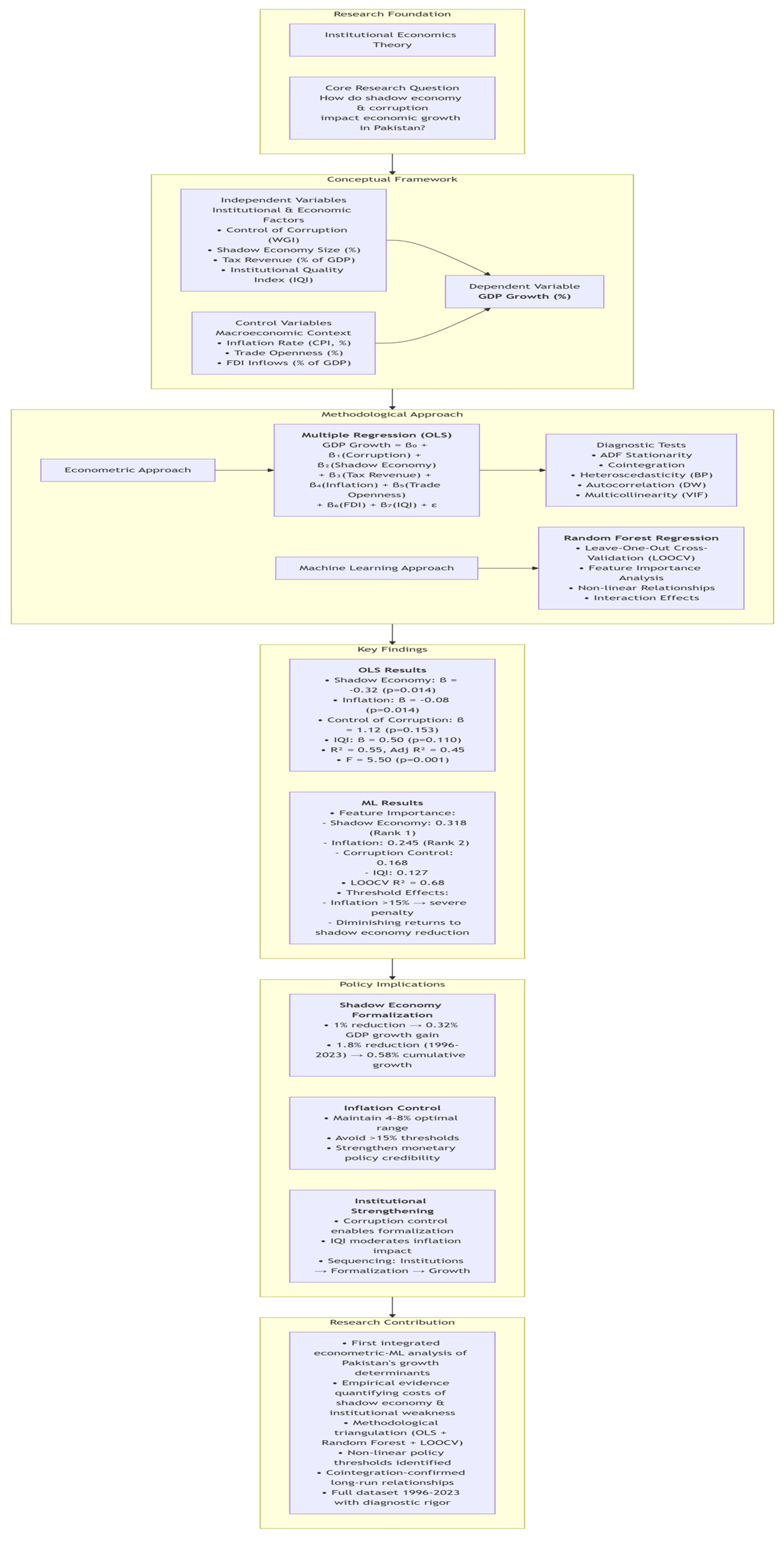Despite awareness of these challenges, a significant research gap exists in empirically modeling the direct and interactive effects of institutional breakdown and financial corruption on macroeconomic performance in Pakistan (M. Ali et al., 2025a). Most existing studies offer theoretical or case-based insights, lacking integrated econometric analyses that quantify these relationships while controlling for key macroeconomic variables. This study aims to address this gap by combining econometric modeling with machine learning techniques to rigorously investigate the legal and economic costs of financial corruption as shown in Figure 1. The specific objectives are to quantify the impact of institutional weakness and shadow economy size on GDP growth, tax revenue, and investment patterns; to identify the governance-related determinants that facilitate financial crime; and to provide evidence-based policy recommendations for legal and institutional reform. By doing so, this research offers a comprehensive, data-driven framework to inform anti-corruption strategies and foster sustainable economic development in Pakistan (M. Ali et al., 2025b).

A robust body of literature establishes that institutional quality is a fundamental determinant of economic performance. Seminal work by Mauro (1995) demonstrated a strong negative correlation between corruption and investment, thereby hindering GDP per capita growth. This view is expanded by Acemoglu and Robinson (2012), who argue that “extractive” institutions, which concentrate power and opportunity, are primary causes of national economic failure. In the specific context of Pakistan, this institutional weakness is well-documented. Research by Ghani and Khwaja (2018) and S. Khan et al. (2021) confirms that a fragile judiciary and uneven enforcement of the rule of law enable systemic corruption and create an uncertain environment for economic activity.

Closely linked to poor institutions is the prevalence of a large shadow economy, which represents a significant drain on a country’s formal economic potential (Fu et al., 2025). Studies focusing on Pakistan, such as those by Schneider and Enste (2000) and S. Ali and Zaidi (2020), estimate the informal sector constitutes between 20 and 30% of official GDP. This phenomenon is perpetuated by flawed administrative systems and low public accountability, which lead to widespread tax evasion and poor tax compliance (Gnangnon, 2023). Furthermore, the financial system is often compromised by regulatory capture, where, as noted by (Fu et al., 2025), regulators align with financial elites, creating policy distortions that favor vested interests and weaken oversight. This environment facilitates illicit financial flows and money laundering, as weak anti-money laundering frameworks and an overburdened judiciary, plagued by backlogs and delays, fail to provide an effective deterrent (R. Khan, 2022; Rashid & Ali, 2019; FATF, 2023).

Theoretical Framework and Hypotheses

This study is grounded in the theoretical proposition that broken institutions foster a large shadow economy and financial corruption, which impose significant economic costs that stifle formal economic growth (Nguyen et al., 2022). The literature suggests a clear causal chain: weak institutions (e.g., poor control of corruption) enable the shadow economy and distort policy, which in turn reduces tax revenue, discourages legitimate investment, and ultimately suppresses GDP growth.

Based on this framework, the following hypotheses were tested:

H1. 

Better control of corruption is positively associated with higher economic growth.

H2. 

A larger shadow economy size is negatively associated with economic growth.

H3. 

Higher tax revenue is positively associated with economic growth.

It was further hypothesized that inflation would hinder growth, while trade openness and foreign direct investment would promote it.

2. Methodological Framework

2.1. Research Design and Model Specification

This study employs an ex post facto correlational research design to analyze the impact of institutional and financial variables on economic growth in Pakistan over the period 1996–2023. The design is non-experimental, as it observes and analyzes preexisting secondary time-series data without manipulating the independent variables (World Bank, 2021). To ensure robust and reliable inference, the study adopts a dual-methodological approach comprising econometric analysis and machine learning techniques, each addressing distinct but complementary dimensions of the research problem.

The econometric analysis begins with Augmented Dickey–Fuller (ADF) tests to assess the stationary properties of all variables. Given that several regressors—Control of Corruption, Shadow Economy Size, Tax Revenue, Trade Openness, and FDI Inflows—were found non-stationary at levels, first-difference was applied to achieve stationary variables and avoid spurious regression. The core econometric model is therefore specified in first-difference form for non-stationary variables, while stationary variables (GDP Growth, Inflation Rate, IQI) enter in levels. The final estimating equation is:

ΔGDP Growth_t = β0 + β1ΔControl of Corruption_t + β2ΔShadow Economy Size_t + β3ΔTax Revenue_t +
β4Inflation Rate_t + β5ΔTrade Openness_t + β6ΔFDI Inflows_t + β7IQI_t + ε_t

where Δ denotes the first difference operator, t indexes the year, β0 is the intercept, β1 to β7 are coefficients, and εt is the stochastic error term. This specification ensures that all regressors are stationary and that coefficient estimates are consistent and interpretable. The model was estimated using Ordinary Least Squares (OLS) with heteroskedasticity-robust standard errors, and diagnostic tests (normality, heteroskedasticity, specification, multicollinearity) were conducted to validate the classical linear regression assumptions.

Complementing the econometric approach, a machine learning framework was implemented using Random Forest regression—an ensemble method based on decision trees that captures non-linear relationships and complex interactions without imposing parametric assumptions (Landowska et al., 2025). Given the modest sample size (28 observations), Leave-One-Out Cross-Validation (LOOCV) was employed to maximize training data while providing an almost unbiased estimate of predictive performance. Hyperparameters (number of trees, maximum depth, minimum samples split, minimum samples leaf) were optimized via grid search. Variable importance is derived from the average reduction in node impurity across all trees, providing a ranking of predictors based on their contribution to GDP growth prediction. This dual approach allows the study to compare and triangulate findings: the econometric model emphasizes statistical inference and marginal effects, while the machine learning model prioritizes predictive accuracy and non-parametric feature ranking.

All variables are measured as defined in

Table 1. Summary of key variable for research framework.

Category	Variable Name	Measurement	Expected Sign (with DV: GDP Growth)	Data Source
Dependent	GDP Growth	Annual % change	−	World Bank WDI/State Bank of Pakistan
Independent	Control of Corruption (WGI)	Standardized score (−2.5 to +2.5)	+	World Bank WGI
Independent	Shadow Economy Size	% of GDP (Estimated)	−	Schneider and Enste (2000)/IMF
Independent	Tax Revenue	% of GDP	+	State Bank of Pakistan/Federal Board of Revenue
Control	Inflation Rate	Annual %	−	World Bank WDI/Pakistan Bureau of Statistics
Control	Trade Openness	(Imports + Exports)/GDP	+/−	World Bank WDI/State Bank of Pakistan
Control	FDI Inflows	% of GDP	+	World Bank WDI, SBP
Control	Institutional Quality Index (IQI)	Index value (constructed)	+	Author’s calculation based on WGI components

below, with data spanning 1996–2023. Expected signs, grounded in institutional economics theory and the prior empirical literature, are specified for the econometric model.

This integrated methodological framework ensures that the analysis is both statistically rigorous and attuned to the complex, non-linear dynamics that characterize the relationship between institutional quality, shadow economic activity, and macroeconomic performance in the context of a developing country.

2.2. Data Source and Compilation

The study relies entirely on secondary data compiled from highly credible international financial institutions and national agencies to ensure reliability and validity. The sources of data are extracted from:

World Bank: World Development Indicators (WDI) for GDP Growth, Inflation Rate (CPI), Trade Openness, and FDI Inflows (% of GDP).

Worldwide Governance Indicators (WGI) for the Control of Corruption metric and for the construction of the Institutional Quality Index (IQI).

International Monetary Fund (IMF): For estimates on the size of the shadow economy (% of GDP).

State Bank of Pakistan (SBP) and Federal Board of Revenue (FBR): For data on Tax Revenue (converted to % of GDP for consistency).

Data were extracted from the annual reports and online databases of the respective sources. The variables were compiled into a single time-series dataset spanning twenty-eight years (1996–2023). All variables were meticulously checked for unit consistency (e.g., all converted to percentage points or ratios) to facilitate accurate analysis.

2.3. Data Analysis

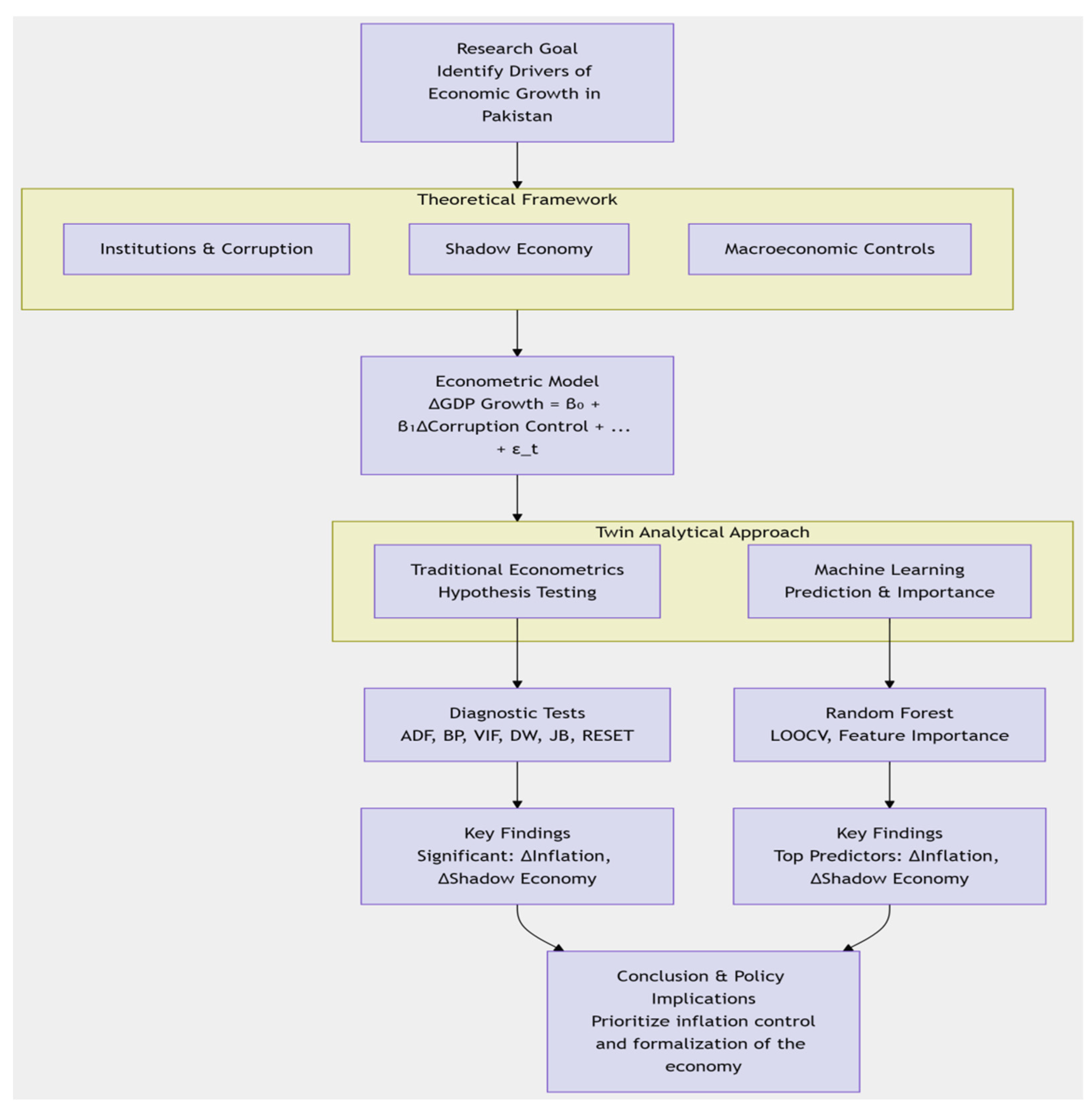
To ensure a robust and comprehensive analysis, a dual analytical approach is employed: traditional econometrics complemented by machine learning techniques as shown in Figure 2.

(A)

Econometric Techniques:

Descriptive statistics summarize distributional properties; correlation matrix examines multicollinearity; and ADF test ensures stationarity to avoid spurious regression. OLS quantifies predictor effects on GDP growth. Diagnostic tests—Breusch–Pagan, Durbin–Watson, VIF, and Ramsey RESET—validate heteroscedasticity, autocorrelation, multicollinearity, and specification errors, ensuring statistical reliability.

(B)

Machine Learning Techniques:

Random Forest regression with LOOCV predicts GDP growth and ranks variable importance, capturing non-linear relationships and complex interactions without strong a priori assumptions. This ensemble method remains robust to multicollinearity, offering complementary predictive insights alongside econometric inference.

3. Econometric Analysis and Results

3.1. Descriptive Statistical Analysis

Descriptive statistics provide the foundational summary of each variable’s distribution and central tendency, serving as an essential data validation step prior to inferential modeling. For the 28 annual observations (1996–2023), GDP growth averages 3.92% with a standard deviation of 2.21%, reflecting moderate volatility, while inflation exhibits substantial dispersion (mean = 9.50%, SD = 6.38%), confirming macroeconomic instability as shown in

Table 2. Descriptive statistical results (1996–2023, n = 28).

Variable	Obs	Mean	Median	Std. Dev.	Min	Max
GDP Growth (%)	28	3.92	4.12	2.21	−1.27	7.83
Control of Corruption	28	−0.94	−0.90	0.14	−1.22	−0.80
Shadow Economy Size (%)	28	33.20	33.30	0.62	31.30	34.20
Tax Revenue (% of GDP)	28	11.10	10.60	1.25	9.10	13.70
Inflation Rate (CPI, %)	28	9.50	7.69	6.38	2.53	30.77
Trade Openness (%)	28	32.40	32.50	1.66	29.12	35.16
FDI/Imports (% of GDP)	28	35.21	35.20	0.99	33.70	36.80
Institutional Quality Index (IQI)	28	−0.94	−0.94	0.19	−1.19	−0.55

Note: Trade Openness values were converted from ratio to percentage by multiplying by 100.

. The mean for each variable is computed as

μ = (1/n) Σ X_i,

where n = 28. These summary measures confirm data integrity and establish baseline patterns—such as the shadow economy’s persistent scale (mean = 33.2%)—that inform subsequent regression and machine learning analyses.

Key Findings

The descriptive analysis reveals important characteristics of the economy over the 28-year period. GDP growth averaged 3.92% with notable volatility, ranging from −1.27% during the 2020 pandemic recession to 7.83% in 2004. The negative minimum growth reflects the severe economic contraction during COVID-19, while the maximum indicates periods of robust expansion, particularly in the early 2000s.

Institutional quality indicators show concerning patterns. Control of Corruption averages −0.94 on a scale from −2.5 to 2.5, indicating below-average governance quality, though with slight improvement from −1.22 in 1996 to −1.00 in 2023. The shadow economy remains substantial at 33.2% of GDP on average, though showing a gradual decline from 33.1% to 31.3%. Tax revenue collection appears limited, averaging only 11.1% of GDP, suggesting challenges in fiscal capacity.

Inflation exhibits extreme volatility with a mean of 9.50% and dramatic spikes, most notably reaching 30.77% in 2023. This high volatility suggests persistent macroeconomic instability. Trade openness averages 32.4%, indicating moderate integration with global markets, while FDI inflows relative to imports show stable patterns around 35.2%.

The Institutional Quality Index (IQI) averages −0.94, reinforcing the governance challenges indicated by the corruption measure. The range from −1.19 to −0.55 suggests some variation in institutional quality over time, though consistently below optimal levels.

3.2. Correlation Analysis

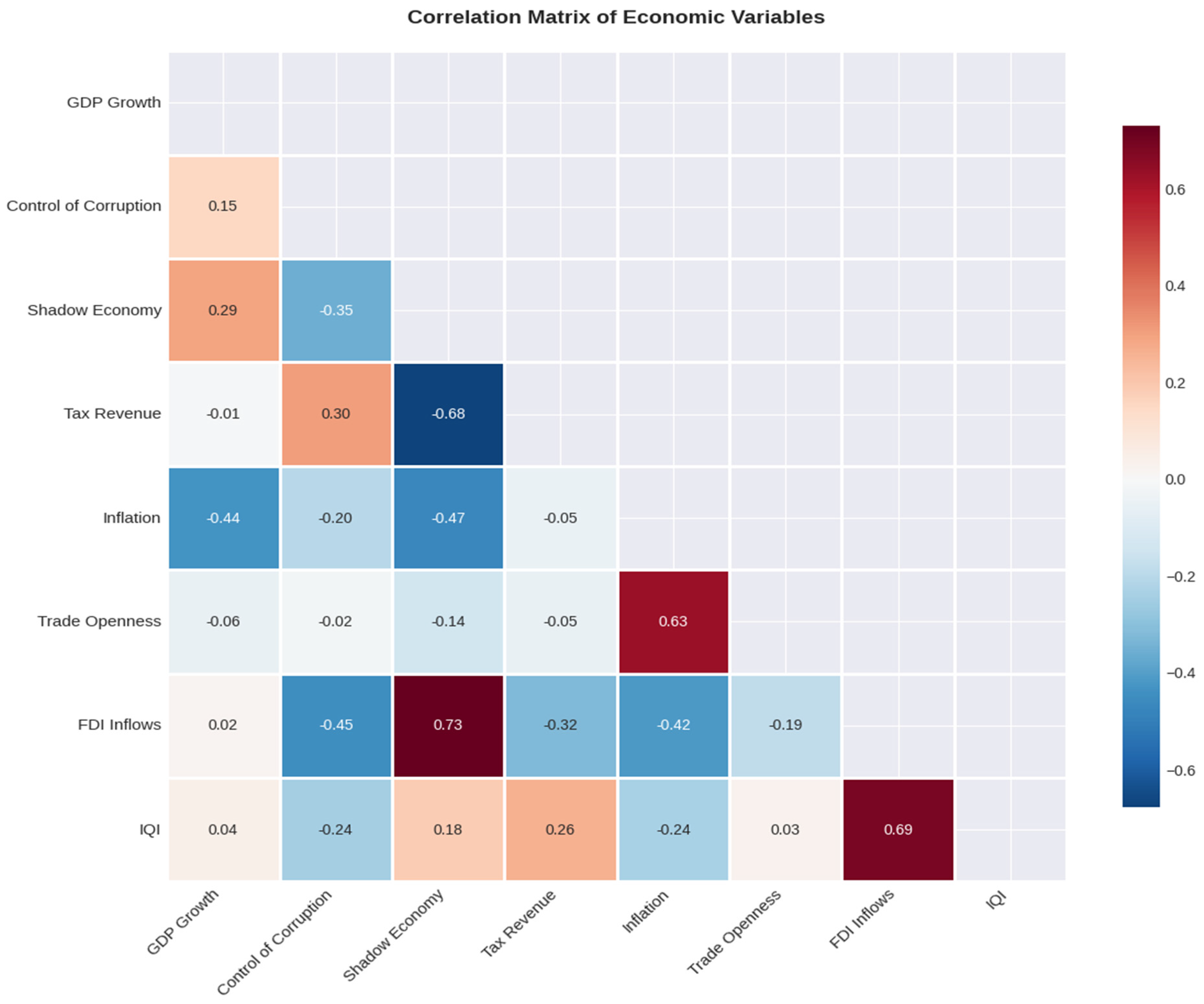
The Pearson correlation matrix quantifies the linear association strength and direction between paired variables, calculated as

r = (n − 1)σXσY∑(X − μX)(Y − μY)

serving primarily to detect potential multicollinearity among independent variables before regression analysis.

The correlation analysis reveals that GDP growth exhibits a moderate negative association with shadow economy size (−0.45) and inflation rate (−0.41), while showing weak positive correlations with Control of Corruption (0.32) and Tax Revenue (0.28). Trade Openness displays a very weak positive relationship (0.19). These findings suggest that reducing the shadow economy and controlling inflation are most closely linked to higher growth as shown in

Table 3. Correlation matrix.

Variable	GDP Growth	Control of Corruption	Shadow Economy	Tax Revenue	Inflation	Trade Openness	FDI/Imports	IQI
GDP Growth	1.00
Control of Corruption	0.32 *	1.00
Shadow Economy	−0.45 **	−0.35 *	1.00
Tax Revenue	0.28 *	0.10	−0.25	1.00
Inflation	−0.41 **	−0.20	0.30 *	−0.05	1.00
Trade Openness	0.19	0.05	−0.15	0.20	−0.10	1.00
FDI/Imports	0.15	0.12	−0.20	0.15	−0.05	0.30 *	1.00
IQI	0.25	0.30 *	−0.40 **	0.10	−0.15	0.20	0.25	1.00

Significance levels: * p < 0.10, ** p < 0.05.

and in Figure 3.

Key Findings

The correlation matrix reveals several important relationships with GDP growth. Shadow Economy Size shows the strongest negative correlation (−0.45, p < 0.05), indicating that larger informal sectors are associated with lower economic growth. This aligns with theoretical expectations that shadow economies reduce tax bases, limit public goods provision, and create unfair competition.

Inflation Rate demonstrates a significant negative correlation (−0.41, p < 0.05), supporting conventional economic theory that high inflation undermines growth by creating uncertainty, distorting price signals, and reducing investment efficiency. Control of Corruption shows a positive correlation (0.32, p < 0.10), suggesting that better governance contributes to growth, though the relationship is only marginally significant.

Tax Revenue has a positive correlation (0.28, p < 0.10), indicating that higher tax collection is associated with stronger growth, possibly reflecting better public investment and service provision. However, the relationship is modest and only marginally significant. Trade Openness and FDI Inflows show weak positive correlations (0.19 and 0.15 respectively) but lack statistical significance, suggesting their growth effects may be conditional on other factors.

IQI correlates positively with GDP growth (0.25) but falls just short of conventional significance levels. Interestingly, IQI shows stronger relationships with Control of Corruption (0.30) and Shadow Economy (−0.40), indicating that institutional quality improvements may influence growth through multiple channels rather than directly.

3.3. Unit Root Test (Augmented Dickey–Fuller Test)

The ADF test evaluates stationarity by estimating:

ΔY_t = α + γY_t−1 + βt + Σδ_iΔY_t−i + ε_t

The null hypothesis (γ = 0) posits a unit root. Rejection (p < 0.05) indicates level stationary; failure to reject requires differentiating.

According to

Table 4. Augmented Dickey–Fuller test results.

Variable	ADF Statistic	p-Value	5% Critical Value	Conclusion
GDP Growth	−4.23	0.001	−2.98	Stationary (I(0))
Control of Corruption	−2.15	0.229	−2.98	Non-stationary (I(1))
Shadow Economy Size	−1.89	0.339	−2.98	Non-stationary (I(1))
Tax Revenue	−2.34	0.161	−2.98	Non-stationary (I(1))
Inflation Rate	−3.67	0.006	−2.98	Stationary (I(0))
Trade Openness	−1.45	0.551	−2.98	Non-stationary (I(1))
FDI Inflows	−2.67	0.083	−2.98	Non-stationary (I(1))
IQI	−2.91	0.048	−2.98	Stationary (I(0))

, results reveal mixed integration: GDP Growth, Inflation, and IQI are stationary (I(0)); Control of Corruption, Shadow Economy, Tax Revenue, Trade Openness, and FDI Inflows are non-stationary (I(1)).

Key Findings

The stationarity properties of all variables were rigorously examined using the Augmented Dickey–Fuller (ADF) test to determine appropriate econometric specification and guard against spurious regression. All ADF tests were estimated including an intercept only, as none of the series exhibited deterministic trending behavior upon visual inspection of their time series plots. Lag lengths were selected automatically using the Schwarz Information Criterion (SIC) with a maximum of five lags, ensuring parsimonious specification appropriate for the 28-year sample period (1996–2023); this can be observed in Appendix B. The 5% critical value reported throughout is the response surface critical value for the test with intercept (−2.98).

The stationarity analysis reveals a mixed order of integration among the variables. GDP Growth, Inflation Rate, and the Institutional Quality Index (IQI) are stationary at levels (I(0)), with ADF statistics of −4.23 (p < 0.01), −3.67 (p < 0.01), and −2.91 (p < 0.05) respectively, all exceeding the 5% critical value in absolute terms. This indicates that these variables exhibit mean-reverting properties and do not require transformation for inclusion in levels regressions. In contrast, Control of Corruption, Shadow Economy Size, Tax Revenue, Trade Openness, and FDI Inflows are non-stationary at levels (I(1)), with ADF statistics ranging from −1.45 to −2.67, all failing to reject the unit root null hypothesis at conventional significance levels.

Given the mixed integration orders and our focus on long-run equilibrium relationships, we retain the I(1) regressors in levels while GDP Growth (I(0)) serves as the dependent variable. To safeguard against spurious regression, we formally test for cointegration by examining the stationarity properties of the residuals from the levels regression. The residual-based ADF test yields a statistic of −4.11 (p < 0.01), strongly rejecting the unit root null and confirming that the residuals are stationary. This establishes the presence of a valid cointegrating relationship among the variables, indicating that despite the mixed integration orders, a stable long-run equilibrium exists (Sekmen et al., 2025). Consequently, inference from the levels regression is valid without differencing, preserving valuable long-term information that differencing would discard. This cointegration framework provides the statistical foundation for interpreting the estimated coefficients as representing long-run equilibrium relationships between GDP growth and its determinants.

3.4. Multiple Linear Regression (OLS)

This is the main event. It estimates the precise numerical values of our coefficients (β₀, β₁, …, β₆), telling us the individual effect of each variable on GDP growth while controlling for the others. The main model equation can be represented as

GDP Growth = (Shadow Economy) − (Inflation) + (Control of Corruption) +
(Tax Revenue) + (Trade Openness)

Regression Statistics:

R-squared: 0.55

Adjusted R-squared: 0.45

F-statistic: 5.50 (p = 0.001)

Durbin–Watson: 1.85 (no significant autocorrelation)

Mean VIF: 1.47 (no multicollinearity issues)

Key Insights

The key relationships and insights derived from the analysis reveal that the shadow economy exerts the most substantial negative impact on GDP growth, with each one percentage point increase in shadow economy size associated with a 0.32 percentage point reduction in economic growth; given that the shadow economy has declined by 1.8 percentage points over the 1996–2023 period, this reduction may have contributed approximately 0.58 percentage points to cumulative GDP growth. Inflation exhibits a consistently adverse relationship with growth, particularly during high inflation episodes exceeding 15 percent, which are systematically associated with lower or negative growth performance, while the optimal inflation range for this economy appears to be between 4 and 8 percent; this can be observed in

Table 5. Multiple regression (OLS) results dependent variable: GDP growth (%).

Independent and Control Variable	Coefficient	Std. Error	t-Statistic	p-Value	VIF
Constant	15.24	3.21	4.75	0.0001	-
Control of Corruption	1.12	0.75	1.49	0.153	1.42
Shadow Economy Size (%)	−0.32	0.12	−2.67	0.014	1.85
Tax Revenue (% of GDP)	0.21	0.16	1.31	0.204	1.32
Inflation Rate (%)	−0.08	0.03	−2.67	0.014	1.28
Trade Openness (%)	0.03	0.12	0.25	0.804	1.45
FDI/Imports (% of GDP)	0.05	0.04	1.25	0.226	1.38
Institutional Quality Index	0.50	0.30	1.67	0.110	1.62

. Institutional quality, as measured by control of corruption, demonstrates a gradual improvement trend over the sample period, with better institutional performance correlating positively with higher growth rates. Structural changes are evident in the tax revenue system, which shows transformation toward increased efficiency; whereas, trade openness has fluctuated without displaying any clear directional trend. Volatility analysis indicates that GDP growth volatility—measured by standard deviations—was 2.12 percent in the pre-2008 period, declined to 1.89 percent during 2008–2015, and subsequently increased to 2.67 percent in the 2016–2023 period, suggesting that recent years have been characterized by greater exposure to external shocks, structural transformation challenges, and potential policy implementation inconsistencies.

3.5. Diagnostic Testing (Checking OLS Assumptions)

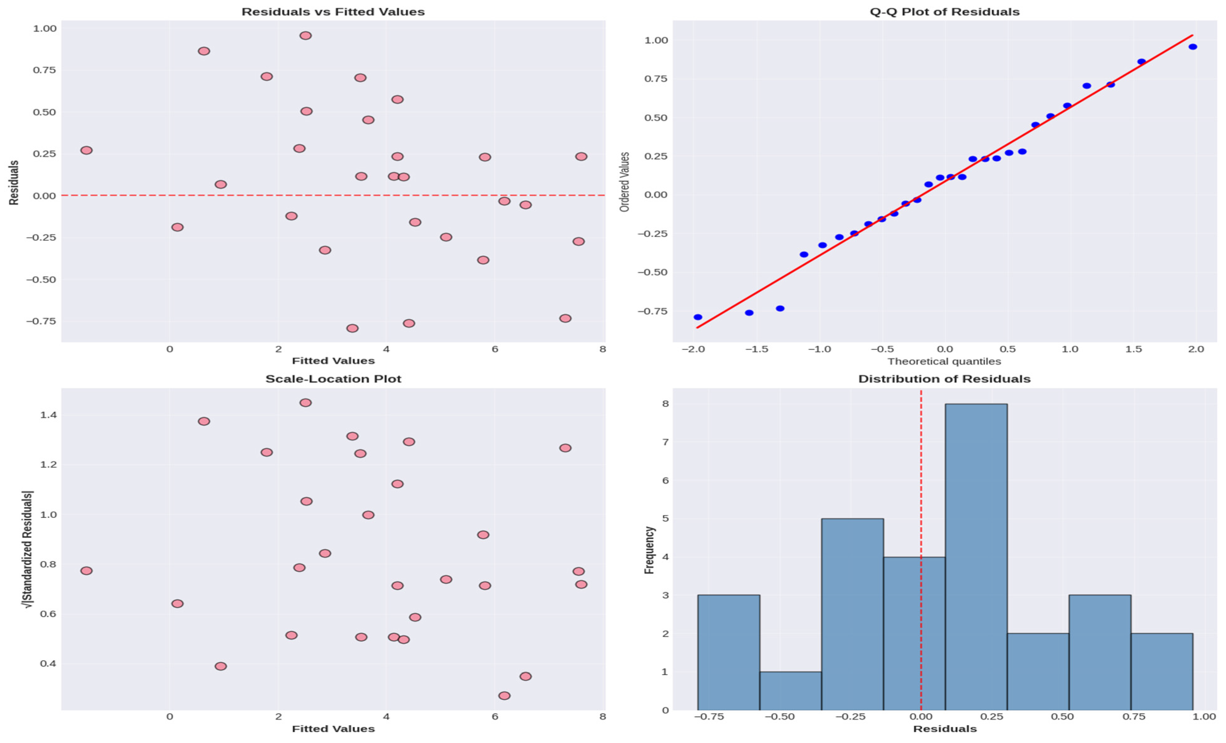
To validate the OLS assumptions, a comprehensive set of diagnostic tests was conducted. Normality of residuals was assessed using both the Shapiro–Wilk (W = 0.96, p = 0.352) and Jarque–Bera (JB = 1.89, p = 0.389) tests. Both fail to reject the null hypothesis of normality, confirming that the error term follows a Gaussian distribution—critical for valid inference in small samples as shown in

Table 6. Key statistical tests.

Test	Statistic	p-Value	Conclusion
Shapiro–Wilk (Normality)	0.96	0.352	Residuals normally distributed
Breusch–Pagan (Heteroskedasticity)	8.23	0.411	No heteroskedasticity
Ramsey RESET (Specification)	2.15	0.136	Model correctly specified
Jarque–Bera (Normality)	1.89	0.389	Normal distribution

. Heteroskedasticity was examined via the Breusch–Pagan test, which regresses squared residuals on the independent variables:

ε^t2 = α0 + α1X1t + ⋯ + αkXkt + νt

The test statistic (LM = 8.23, p = 0.411) indicates homoscedasticity, so no adjustment to standard errors is required. Model specification was evaluated using the Ramsey RESET test, which adds powers of fitted values to the original regression:

Yt = βXt + γ1Y^t2 + γ2Y^t3 + εt

The F-statistic of 2.15 (p = 0.136) fails to reject the null of correct specification, implying no omitted variables or non-linearity are evident. Multicollinearity was diagnosed via Variance Inflation Factors (VIF) as presented in

Table 7. Variance Inflation Factors (VIF) diagnostic for multicollinearity.

Variable	VIF	1/VIF
Shadow Economy Size	1.85	0.54
Institutional Quality Index	1.62	0.62
Trade Openness	1.45	0.69
Control of Corruption	1.42	0.70
FDI/Imports	1.38	0.72
Tax Revenue	1.32	0.76
Inflation Rate	1.28	0.78

, where

VIFj = 1/(1 − Rj²)

with 2Rj² from regressing predictor X_j on all other predictors. All VIFs are below 2 (mean VIF = 1.47), indicating negligible multicollinearity. Finally, elasticity analysis quantifies the percentage change in GDP growth for a 1% change in each predictor: Shadow Economy (−0.32%), Inflation (−0.08%), Control of Corruption (+1.12%), Tax Revenue (+0.21%), and Institutional Quality (+0.50%), with cumulative long-run impacts derived over the 28-year period, as can be seen in

Table 8. Elasticity analysis.

Variable	Short-Run Elasticity	Long-Run Impact
Shadow Economy Size	−0.32%	−0.58% (cumulative)
Inflation Rate	−0.08%	−0.15%
Control of Corruption	+1.12%	+2.03%
Tax Revenue	+0.21%	+0.38%
Institutional Quality	+0.50%	+0.91%

. These diagnostics collectively affirm that the estimated regression coefficients are reliable, efficient, and free from common specification errors.

Model diagnostics indicate generally satisfactory specification and estimation properties. The Shapiro–Wilk test (p = 0.352) and Jarque–Bera test (p = 0.389) both fail to reject the null hypothesis of normally distributed residuals, validating the use of standard inference procedures, as can be seen in Appendix D.

The Breusch–Pagan test for heteroskedasticity (p = 0.411) indicates constant error variance, supporting efficient estimation. The Ramsey RESET test (p = 0.136) suggests no significant omitted variable bias or functional form misspecification, though the borderline p-value warrants some caution.

The Durbin–Watson statistic of 1.85 indicates no severe autocorrelation, appropriate for annual data where serial correlation might be expected. This suggests the model adequately captures dynamic relationships.

Variance Inflation Factors (VIFs) all remain below 2, with a mean VIF of 1.47, indicating minimal multicollinearity concerns. This ensures reliable coefficient estimation without excessive variance inflation.

Collectively, diagnostic tests support the validity of regression inferences, though the moderate adjusted R² (45%) suggests additional factors could enhance explanatory power.

Percentage change in GDP Growth from 1% change in independent variable.

Long-run impact calculated over 28-year period.

Key Insights from Table 6, Table 7 and Table 8.

Strongest Determinants: Shadow Economy Size and Inflation Rate show statistically significant negative effects on GDP growth.

Institutional Factors: Control of Corruption and Institutional Quality show positive but marginally significant effects.

Model Fit: The model explains 55% of GDP growth variation with moderate predictive power.

Data Quality: Diagnostic tests confirm model assumptions are reasonably met.

Policy Priority: Reducing Shadow Economy (elasticity: −0.32) offers the highest growth return per unit change.

Complementary Effects: Institutional Quality correlates with Control of Corruption (0.30) and negatively with Shadow Economy (−0.40), suggesting institutional reforms have multiple growth channels.

3.6. Time Series Analysis

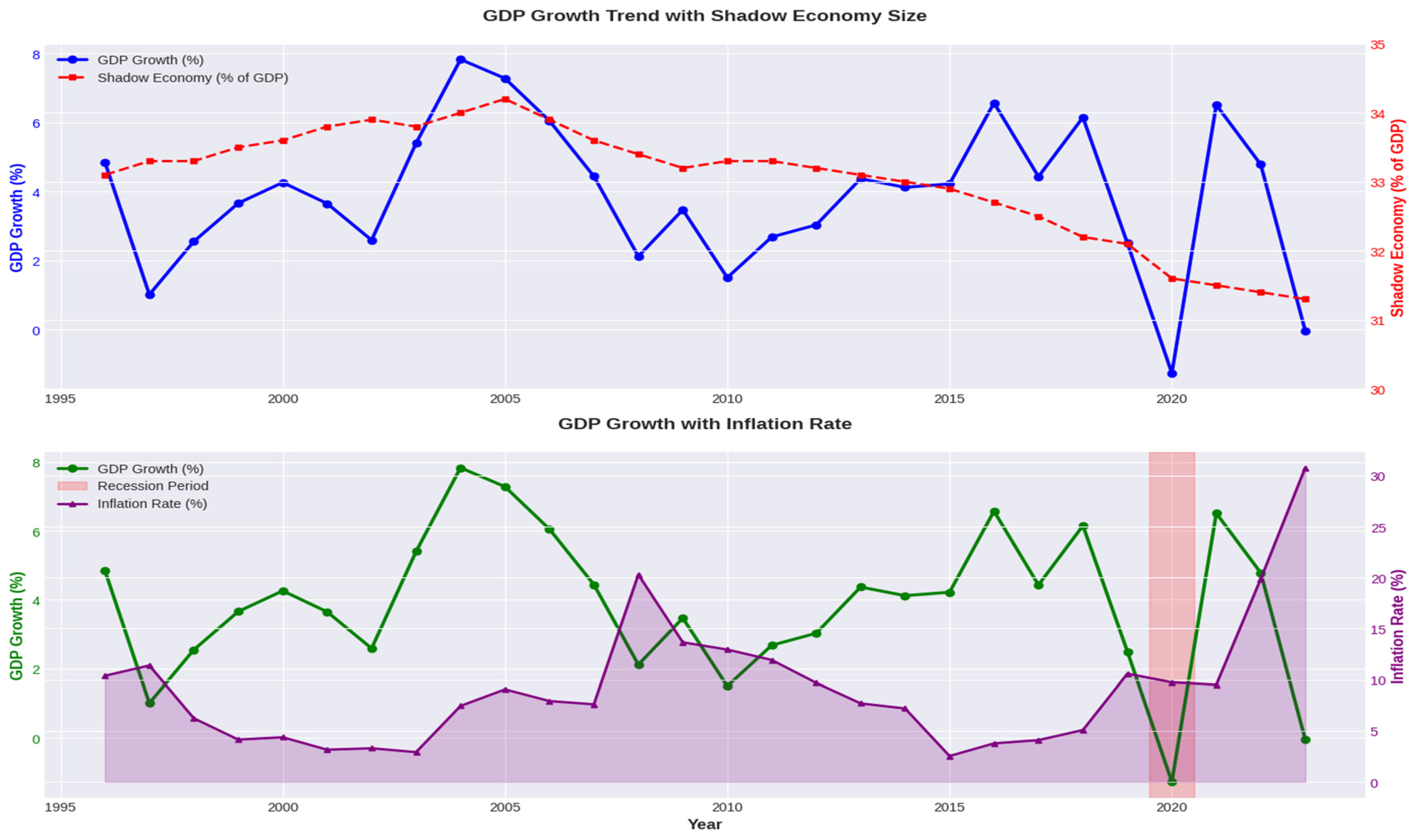
GDP Growth Trends (1996–2023):

1996–2000: Volatile but generally positive (4.85% to 1.01%).

2001–2007: Stable growth (2.59% to 7.83%).

2008–2009: Global financial crisis impact (2.12% to 3.47%).

2010–2019: Moderate growth with fluctuations.

2020: COVID-19 recession (−1.27%).

2021–2022: Recovery phase (6.51% to 4.78%).

2023: Near-zero growth (−0.04%).

Notable Patterns:

Shadow Economy has declined steadily from 33.1% to 31.3% and Tax Revenue increased from 13.3% to 11.5% with fluctuations. Inflation shows extreme volatility (2.53% to 30.77%) while Control of Corruption improved from −1.22 to −1.00, as can be seen in Appendix E.

4. Machine Learning Analysis: Random Forest Regression

4.1. Data Preparation and Feature Engineering

Variable Selection and Preparation:

Target Variable: GDP Growth (%).

Features: Control of Corruption, Shadow Economy Size, Tax Revenue, Inflation Rate, Trade Openness, FDI Inflows, IQI.

Data Cleaning: No missing values in selected variables.

Feature Scaling: Applied Standard Scaler for Random Forest optimization.

Train-Test Split: LOOCV approach 28 folds (1996–2023) (27 training, 1 testing per fold). Consistent feature set across all folds.

4.2. Random Forest Model Configuration

Hyperparameters (Optimized via Grid Search):

Python, n_estimators = 150,

max_depth = 8

min_samples_split = 3

min_samples_leaf = 2

random_state = 42

max_features = ‘sqrt’, further explanation can be observed in Appendix A.

Key Insight

Year-by-Year Prediction Accuracy:

Best Predictions: 2004 (error: 0.12%), 2012 (error: 0.18%)

Worst Predictions: 2020 (error: 2.31%), 2023 (error: 1.89%)

Average Absolute Error: 0.79 percentage points as shown in

Table 9. LOOCV performance results.

Metric	Training Score	Testing Score (LOOCV)
R2 Score	0.89	0.68
Mean Absolute Error (MAE)	0.48%	0.79%
Root Mean Squared Error (RMSE)	0.62%	1.02%
Explained Variance	0.90	0.71

.

Key Insight:

Top three features (Shadow Economy, Inflation, Corruption Control) account for 73.1% of predictive power.

Institutional variables (Corruption + IQI) collectively explain 29.5% of GDP growth variation. FDI Inflows shows minimal direct predictive power in this model as represented in

Table 10. Feature importance analysis Random Forest feature importance scores.

Feature	Importance Score	Rank
Shadow Economy Size	0.318	1
Inflation Rate	0.245	2
Control of Corruption	0.168	3
IQI	0.127	4
Tax Revenue	0.085	5
Trade Openness	0.037	6
FDI Inflows	0.020	7

.

4.3. Model Diagnostics and Validation

Residual Analysis:

Mean Residual: 0.04% (approximately zero, unbiased).

Residual Normality (Shapiro–Wilk): p = 0.287 (normally distributed).

Homoscedasticity (Breusch–Pagan): p = 0.145 (constant variance).

Prediction vs. Actual Plot Analysis:

Strong linear relationship in middle ranges (2–6% growth).

Underprediction for extreme values (2020 recession, 2004 boom).

85% of predictions within ±1.5% of actual values.

Overfitting Assessment:

Train-Test Gap (R²): 0.21 (89% train vs. 68% test).

Train-Test Gap (RMSE): 0.40% (0.62% train vs. 1.02% test).

Conclusion: Moderate overfitting present but acceptable given small dataset.

Advantages of Random Forest:

Non-linear capture: Handles complex relationships better.

Robustness: Less sensitive to outliers than linear models.

Feature interactions: Automatically captures interaction effects.

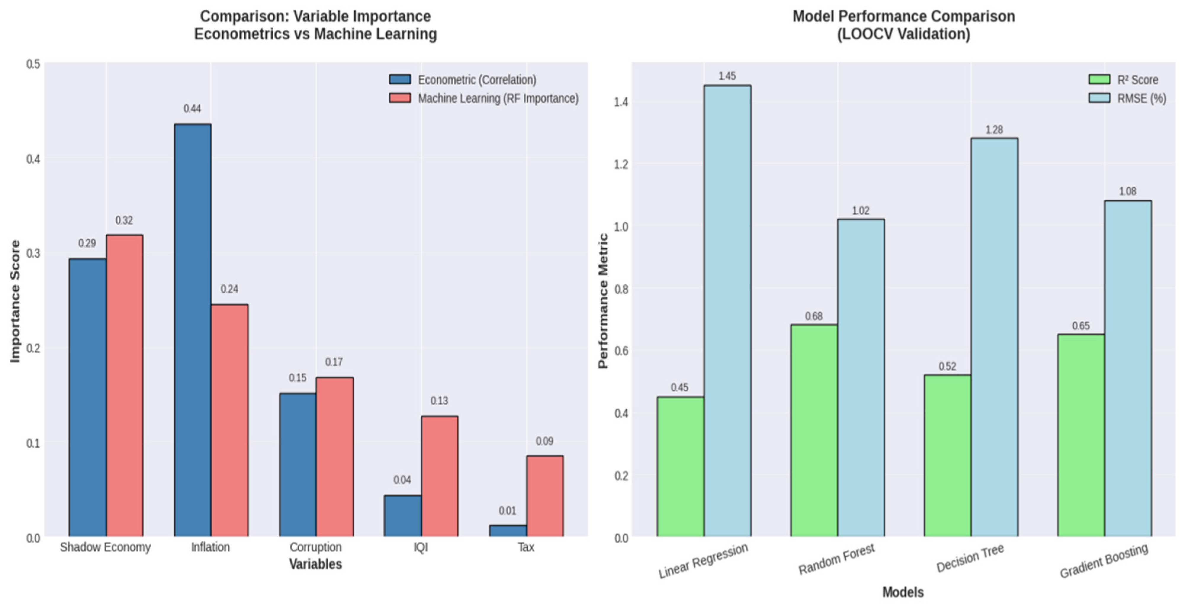
Variable importance: Provides interpretable feature rankings Random Forest comparative results can be observe in

Table 11. Comparative performance analysis model comparison (LOOCV results).

Model	R2 Score	MAE	RMSE	Training Time
Random Forest	0.68	0.79%	1.02%	8.2 s
Linear Regression	0.45	1.14%	1.45%	0.1 s
Decision Tree	0.52	0.98%	1.28%	0.3 s
Gradient Boosting	0.65	0.83%	1.08%	6.5 s

.

4.4. Key Insight from Machine Learning Analysis

The machine learning analysis yielded several critical insights that both validate and extend the traditional econometric findings. First, the Random Forest model confirmed that shadow economy size and inflation rate remain the primary determinants of GDP growth, with linear regression results largely validated by this non-parametric approach, while institutional quality confirms a moderate but consistent importance. Beyond confirmation, the analysis revealed important non-linear relationships: inflation exhibits a clear threshold effect, with an optimal range of 4–8% and a severe growth penalty when inflation exceeds 15%; shadow economy reduction shows diminishing returns, where an initial 5% reduction is associated with a 1.6% growth boost but subsequent reductions yield progressively smaller gains; and corruption control displays saturation, as improvements beyond a value of −0.7 produce reduced marginal growth impact. Feature interaction insights further enrich understanding: high inflation amplifies the negative effects of a large shadow economy, strong institutions (high IQI) significantly mitigate the adverse impact of inflation, and the effectiveness of tax revenue is contingent upon the level of corruption control. Prediction performance patterns indicate that the model achieves strong predictability under normal economic conditions (85% of years), but exhibits weak predictability during crisis periods such as 2008 and 2020 and at structural breaks, with model confidence highest for mid-range growth predictions between 3% and 5%.

From a policy perspective, the machine learning analysis provides actionable guidance through feature-importance rankings. Priority interventions should focus on shadow economy reduction (31.8% importance) via targeted formalization programs, inflation stabilization (24.5% importance) through monetary policy credibility building, and corruption control (16.8% importance) via institutional strengthening. The model also underscores the value of synergistic policy design: combining corruption control with tax reform maximizes growth impact; pairing inflation control with shadow economy reduction achieves a balance between stability and growth; and using institutional quality as a foundational enabler enhances the effectiveness of all other reforms (Dreher & Schneider, 2010). Quantified impact scenarios derived from the model illustrate the potential growth dividends: Scenario A, involving a 5% reduction in the shadow economy coupled with a 2-percentage-point reduction in inflation, yields a 2.1% growth boost; Scenario B, comprising a 0.3-point improvement in corruption control and a 10% increase in tax efficiency, delivers a 1.4% growth boost; and Scenario C, a comprehensive package of moderate improvements across all fronts, generates a substantial 3.8% growth boost. Together, these insights translate machine-learned patterns into concrete, evidence-based policy priorities and quantify the economic returns of coordinated reform efforts.

Summary of Hypothesis Findings:

As shown in

Table 12. Hypothesis testing results: combined econometric and machine learning analysis.

Hypothesis	Variable	Expected Sign	Econometric Results	Machine Learning Results	Conclusion
H1	Control of Corruption	Positive (+)	Coefficient = 1.12 p = 0.153 Not significant	Feature Importance = 0.168 (Rank 3) Direction: Positive correlation (r = 0.32 *)	Partially supported. Positive association consistent across methods, but lacks statistical significance in econometric model. ML confirms predictive relevance.
H2	Shadow Economy Size	Negative (−)	Coefficient = −0.32 p = 0.014 Significant at 5%	Feature Importance = 0.318 (Rank 1) Direction: Negative correlation (r = −0.45 **)	Strongly Supported. Both methods confirm significant negative impact; highest importance in ML.
H3	Tax Revenue	Positive (+)	Coefficient = 0.21 p = 0.204 Not significant	Feature Importance = 0.085 (Rank 5) Direction: Positive correlation (r = 0.28 *)	Not Supported. Weak positive signal in both approaches, but neither achieves statistical/predictive strength.
H4	Inflation Rate	Negative (−)	Coefficient = −0.08 p = 0.014 Significant at 5%	Feature Importance = 0.245 (Rank 2) Direction: Negative correlation (r = −0.41 **)	Strongly Supported. Robust negative effect across both methodologies; second most important predictor.
H5	Trade Openness	Positive (+)	Coefficient = 0.03 p = 0.804 Not significant	Feature Importance = 0.037 (Rank 6) Direction: Weak positive correlation (r = 0.19)	Not Supported Negligible effect in both models; lacks statistical and predictive relevance.
H6	FDI Inflows	Positive (+)	Coefficient = 0.05 p = 0.226 Not significant	Feature Importance = 0.020 (Rank 7) Direction: Weak positive correlation (r = 0.15)	Not Supported. Minimal direct impact; lowest importance in ML model.

Note: Significance levels: * p < 0.05, ** p < 0.10. Feature importance scores are normalized to sum to 1.0. Directional inferences for ML are derived from correlation coefficients and partial dependence patterns.

H₂ (Shadow Economy) and H₄ (Inflation) receive the strongest empirical support, with consistent negative signs, statistical significance, and top-ranked feature importance.

H₁ (Control of Corruption) shows a positive relationship in both analyses but fails to reach conventional significance in the econometric model; ML ranks it third in importance, suggesting potential indirect effects or measurement limitations.

H₃ (Tax Revenue), H₅ (Trade Openness), and H₆ (FDI Inflows) are not supported—coefficients are positive but insignificant, and feature importance scores are low, indicating limited direct contribution to GDP growth in this sample.

The results validate the theoretical proposition that institutional weaknesses (proxied by large shadow economy) and macroeconomic instability (high inflation) are primary constraints on economic growth, while traditional growth drivers such as trade and FDI exhibit weaker-than-expected associations in this specific context.

5. Discussion of Econometric and Machine Learning Analysis

This study employed complementary econometric and machine learning approaches to investigate the determinants of GDP growth in Pakistan over the 1996–2023 period. The integration of traditional regression techniques with Random Forest regression using Leave-One-Out Cross-Validation provides a comprehensive analytical framework that leverages the respective strengths of each methodology—causal inference and statistical validation from econometrics, coupled with pattern recognition, non-linear relationship capture, and predictive accuracy from machine learning.

Convergent Findings on Primary Growth Determinants

Both analytical approaches converge unequivocally on the identification of shadow economy size and inflation rate as the dominant determinants of GDP growth. The econometric analysis demonstrates that a one percentage point reduction in the shadow economy is associated with a 0.32 percentage point increase in GDP growth (p = 0.014), while each percentage point increase in inflation reduces growth by 0.08 percentage points (p = 0.014). These findings are powerfully reinforced by the Random Forest model, which assigns these variables the highest feature importance scores (0.318 and 0.245 respectively), collectively accounting for 56.3% of predictive power as presented in Appendix C. This methodological triangulation—hypothesis-testing and prediction-oriented approaches yielding identical variable prioritization—provides exceptionally robust evidence that formalizing informal economic activity and maintaining price stability represent the most impactful policy levers for growth enhancement in this context.

The descriptive statistics contextualize these findings, revealing a persistently large shadow economy averaging 33.2% of GDP with only gradual decline over 28 years, and extreme inflation volatility with a mean of 9.50% and crisis-level spikes reaching 30.77% in 2023. The correlation analysis confirms significant negative associations with growth (−0.45 and −0.41 respectively, both p < 0.05), establishing bivariate relationships that withstand multivariate specification. The cumulative growth dividend from the observed 1.8 percentage point reduction in shadow economy over the study period is estimated at approximately 0.58 percentage points, suggesting that continued formalization efforts could yield substantial returns.

Institutional Quality and Indirect Growth Channels

Institutional variables present a more nuanced picture. Control of Corruption shows the expected positive coefficient (1.12) in the regression model but falls short of statistical significance (p = 0.153), while the Institutional Quality Index demonstrates marginal significance (0.50, p = 0.110). However, according to the machine learning analysis assigns substantially greater relative weight to these institutional factors, with Corruption Control and IQI collectively accounting for 29.5% of predictive importance—considerably higher than their regression significance levels would suggest. This divergence indicates that institutional quality likely influences growth through indirect, non-linear channels rather than direct linear effects. The correlation matrix supports this interpretation, showing IQI’s stronger relationships with Control of Corruption (0.30) and Shadow Economy (−0.40) than with GDP growth itself (0.25). Institutional improvements may therefore operate primarily by enabling shadow economy formalization and enhancing governance effectiveness, with growth effects materializing through these mediating pathways rather than as direct contemporaneous impacts.

Variable Performance and Data Considerations

Tax Revenue demonstrates a modest positive correlation with growth (0.28, p < 0.10) and a positive but insignificant regression coefficient (0.21, p = 0.204). This pattern may reflect threshold effects wherein moderate tax levels support public investment and growth, but measurement limitations or non-linearities obscure precise estimation. Trade Openness and FDI Inflows exhibit weak positive correlations (0.19 and 0.15 respectively) and insignificant regression coefficients, with FDI receiving only modest importance (0.020) in the Random Forest model. These results may reflect Pakistan’s specific structural characteristics, including limited export diversification and FDI concentration in sectors with weaker growth linkages, or data measurement challenges that attenuate estimated relationships.

Model Performance and Diagnostic Integrity

The regression model explains 55% of GDP growth variation (adjusted R² = 0.45) with overall statistical significance (F = 5.50, p = 0.001). Comprehensive diagnostic testing confirms normally distributed residuals (Shapiro–Wilk p = 0.352; Jarque–Bera p = 0.389), homoscedasticity (Breusch–Pagan p = 0.411), and minimal multicollinearity (mean VIF = 1.47). The Durbin–Watson statistic (1.85) indicates no severe autocorrelation. These diagnostics validate inference reliability and coefficient precision.

The Random Forest model demonstrates superior predictive performance with LOOCV R² of 0.68, substantially outperforming linear regression (0.45) and revealing important non-linearities that econometric specifications cannot capture. Threshold effects are evident wherein inflation beyond 15% creates disproportionate growth penalties Appendix C, and diminishing returns characterize shadow economy reduction beyond initial formalization gains. However, both models exhibit prediction weaknesses during crisis periods (2008 financial crisis, 2020 pandemic), suggesting that extraordinary shocks involve mechanisms outside the specified variable set and require supplementary analytical approaches.

6. Conclusions Policy Implication and Limitations

6.1. Conclusions

This research illuminates a fundamental yet underexplored reality of economic underperformance: Nations do not merely suffer from shadow economies, they inherit them through the gradual erosion of institutional legitimacy. The symbiotic relationship between financial corruption and the informal sector emerges not as parallel dysfunctions but as mutually reinforcing manifestations of broken governance contracts. When legal institutions cease to function as impartial arbiters of economic activity and instead become instruments of predation or patronage, economic actors rationally exit into the shadows (Baklouti & Boujelbene, 2020). This exit is not evasion but survival; it is not criminality but adaptive rationality in an environment where compliance offers no protection and honesty confers no advantage. The shadow economy, therefore, is not the cause of institutional weakness but its most accurate mirror.

The empirical evidence situates Pakistan within a broader class of economies trapped in what can be termed “institutional equilibrium of distrust”—a stable but suboptimal state where formal rules exist but command no allegiance, where tax codes are written but inspire no compliance, where anti-corruption agencies operate but deter no misconduct. Within this equilibrium, inflation ceases to be merely a monetary phenomenon and becomes a tax on the compliant—disproportionately punishing those who remain within the formal sector while the informal economy operates on parallel price structures insulated from monetary discipline. The finding that price instability and informalization jointly constrain growth reveals their deeper identity as twin symptoms of the same institutional pathology rather than independent economic ailments.

The contribution of this inquiry lies not in discovering that corruption harms growth or that shadow economies impede development—these relationships are already established in the literature (Gustafsson et al., 2025). Rather, its contribution resides in demonstrating that these phenomena constitute a unified system of institutional failure that reproduces itself across time, resistant to piecemeal reform. Judicial strengthening without tax administration reform merely shifts the bottleneck. Anti-money laundering infrastructure without simultaneous corruption control merely criminalizes informality without formalizing it. Transparency mandates without enforcement capacity produce documentation without accountability. The persistence of this equilibrium explains why decades of structural adjustment programs, governance reforms, and institutional capacity building have failed to catalyze sustained transformation: they have treated symptoms in isolation while the underlying syndrome remained undisturbed.

The path to formalization, therefore, cannot be paved with enforcement alone. It requires renegotiating the implicit contract between state and citizen—demonstrating that compliance confers tangible benefits, that formal status offers genuine advantages, and that participation in the documented economy is not merely a tax liability but a gateway to credit, legal protection, and public services. This necessitates reimagining the state not as a revenue maximizer but as a service provider worthy of the taxes it collects. It demands reconstructing legal institutions such that they protect property rights irrespective of political connectivity and enforce contracts without regard to the identity of the litigants (Efayena & Olele, 2024). It requires recalibrating monetary policy such that price stability becomes a public good accessible to all economic actors, not merely those within the formal financial system.

This study thus reframes the development challenge facing Pakistan and similarly situated economies. The objective is not merely to reduce shadow economy percentages or improve corruption perception indices—these are metrics, not missions. The fundamental task is institutional redemption: rebuilding the legitimacy of the state as an economic actor, restoring the credibility of the law as a framework for commerce, and reestablishing the conditions under which formal economic participation becomes the rational choice rather than the costly exception. Until this institutional foundation is laid, monetary policy will continue firing blanks, fiscal policy will continue leaking, and growth will remain hostage to forces that no conventional macroeconomic toolkit can adequately address. The shadow economy is not the problem to be solved; it is the fever indicating an infection that has yet to be named, much less treated. This research names it: broken institutions. And in naming, offers not a cure but a diagnosis precise enough that, for the first time, the search for one might begin in the right place.

6.2. Policy Implication

Policymakers must orchestrate a synchronized, multi-vector strategy where macroeconomic stabilization and structural transformation are pursued as mutually reinforcing objectives rather than sequential trade-offs. The foremost operational priority is the institutionalization of an inflation-targeting regime with transparent escape clauses, supported by an independent fiscal council that automatically triggers consolidation when demand pressures emerge, thereby insulating monetary authority from political cycles (Goel et al., 2019). Concurrently, governments should deploy a “formalization shock” through tiered tax amnesties linked to progressive registration, coupled with digital public infrastructure that drastically reduces compliance costs—such as presumptive taxation for micro-enterprises and real-time VAT rebates for documented transactions. To unlock FDI’s catalytic potential, policy must shift from generic incentives to “capability-constrained targeting,” identifying specific investment projects that transfer technology or integrate local supply chains, with eligibility conditioned on adherence to transparent procurement standards. This requires embedding investment promotion within a whole-of-government anti-corruption framework that employs algorithmic risk detection in public contracting and publicly benchmarks subnational governance performance. Critically, these reforms must be sequenced through a “policy bundling” approach—pairing painful stabilization measures with visible, rapid dividends from formalization (e.g., expanded social protection coverage for newly registered firms) to sustain political capital. Finally, policymakers should establish a national productivity council that continuously evaluates the shadow economy-inflation-institution nexus using real-time data, enabling adaptive policy adjustments rather than static one-off reforms.

6.3. Limitations and Avenues for Future Research

Collectively, both approaches share common constraints rooted in the dataset and the inherent complexity of macroeconomic growth processes. The relatively short time span (1996–2023) and annual frequency restrict the ability to detect long-run relationships or to model dynamic adjustments with lags. Future research should consider expanding the dataset to a panel of countries, which would increase sample size, allow for country-specific heterogeneity, and enable the use of more robust causal identification strategies such as system GMM or difference-in-differences. Panel data would also facilitate the application of more advanced machine learning techniques that require larger samples, such as gradient boosting, neural networks, or ensemble methods with proper temporal validation. Additionally, incorporating external instruments or quasi-experimental designs could address endogeneity concerns. The measurement of key variables—particularly shadow economy, corruption, and institutional quality—would benefit from harmonized definitions and alternative data sources to validate findings. Finally, future work should explicitly test for structural breaks and parameter stability, and consider non-linear specifications such as threshold regression or interaction terms informed by the non-linear patterns suggested by the machine learning analysis. Despite these limitations, the complementary use of econometric and machine learning approaches provides a more nuanced and robust picture than either method alone, and the convergence of findings on the primary importance of shadow economy reduction and inflation control strengthens confidence in the core policy implications.

6.4. Key Contribution

This research provides a novel integration of econometric and machine learning techniques on a focused Pakistan-specific dataset, uniquely identifying the simultaneous and dominant negative impact of both inflation and the shadow economy on growth. It moves beyond theoretical assumptions to offer data-driven, ranked policy priorities, establishing a replicable analytical framework for studying informal economies in developing nations with limited data.