Investigating the Relationship Between Liquidity Risk, Credit Risk, and Solvency Risk in Banks Listed on the Iranian Capital Market: A Panel Vector Error Correction Model

Abstract

In the aftermath of global financial crises and amid increasing complexity in banking operations, understanding and managing various types of risk—especially liquidity, credit, and solvency risks—has become a global concern for financial stability. This study addresses a critical gap in the literature by examining the dynamic interrelationships among these three types of risk in the context of emerging markets. Using data from 21 banks listed on the Iranian capital market from 2011 to 2023, we employ a Panel Vector Error Correction Model (VECM) alongside panel impulse response analysis to assess both short- and long-term dynamics. Our results reveal that an increase in liquidity positively impacts bank solvency, while credit risk negatively affects solvency but does not significantly influence liquidity risk. These findings contribute to the theoretical understanding of systemic risk interactions in banking and provide practical insights for policymakers and financial institutions seeking to enhance risk management strategies in volatile market environments.

1. Introduction

In recent decades, global financial systems have experienced repeated disruptions—most notably the 2008 financial crisis and the more recent challenges triggered by the COVID-19 pandemic. These events have highlighted the central role of financial institutions, especially banks, in both exacerbating and mitigating systemic risk. Amid such turbulence, ensuring the stability and resilience of the banking sector has become a global priority. This has increased attention to the complex interplay of major financial risks, especially liquidity risk, credit risk, and solvency risk.

Despite the global relevance of these risks, empirical studies in emerging markets—particularly Iran—remain limited. Iran’s banking sector, under the pressure of prolonged economic sanctions, currency fluctuations, and regulatory constraints, presents a unique case for investigating how these risks interact. According to recent financial reports, several Iranian banks have experienced declining capital adequacy ratios and rising non-performing loans, raising concern about potential systemic vulnerabilities. However, the nature and direction of interdependencies between key risks have not yet been clearly identified.

The banking industry has always been associated with various complications and risks and has gone through multiple economic crises. In this complex industry, the stability, growth, and flexibility of the banks have consistently been key concerns for bank managers and economic policymakers, especially considering the turbulent economic conditions. Risk analysis and its management is a process that helps organizations, especially financial institutions, to predict, understand, and manage both systemic and internal risk (Zhang et al., 2023; Peykani et al., 2023a; Varma et al., 2022; Bhimjee et al., 2016). Risk management in organizations enables managers to improve organizational performance by minimizing losses and maximizing profits. Banks are among the most important institutions operating in global financial and monetary markets, and they are exposed to a wide range of risks. Due to the direct relationship between banks and all segments of society—particularly following the 2008 global financial crisis and more recent events such as the COVID-19 pandemic—the necessity of risk management in banks and financial institutions has become a critical concern worldwide and is now being pursued with increased urgency (Ding & Wei, 2023; Adam et al., 2023; Telg et al., 2023; Galletta et al., 2023).

Due to the large social, financial, and economic dimensions of the inappropriate performance of some banks, excessive exposure of banks to financial risks can cause bankruptcy and have significant impacts on the lives of many people (Peykani et al., 2023b; Berger & Demirgüç-Kunt, 2021; Lin & Han, 2021; Anton & Nucu, 2020). By understanding the risks facing banks, governments can set better regulations to encourage prudent management and rational decision-making (Mateev et al., 2023; Hoque et al., 2015; Laeven & Levine, 2009; González, 2005). It is also important to state that a bank’s ability to manage risk affects investors’ decisions. Even if banks can generate a lot of income, their lack of risk management can severely reduce profits due to loan losses and negatively affect the bank’s overall performance in terms of profitability. It should be noted that experienced investors invest more in a bank that has the ability to finance and provide profit and is perceived as being at a low risk of financial loss (Breitenstein et al., 2021; Park & Jang, 2021; J. Wang et al., 2021).

The most important risks in banks are credit risk and liquidity risk, which if neglected or improperly managed will lead to irreparable social, political and economic consequences (Von Tamakloe et al., 2023; Affandi et al., 2023; Rezvani et al., 2023; Cahyandari et al., 2023). Understanding the various types of risks within banking systems helps institutions develop effective risk management strategies. Since banks are exposed to various risks, they have appropriate risk management infrastructures and are required to comply with government regulations, which are typically designed to mitigate risks and protect depositors (Adam et al., 2023; Ding & Wei, 2023; Cornwell et al., 2023).

Credit risk is the biggest risk in banking, and it happens when borrowers do not fulfill their contractual obligations and default in paying their loans’ principal or interest. Defaults can occur on mortgages, credit cards, fixed income securities, and derivatives (Pozo & Rojas, 2023; Telg et al., 2023; Noriega et al., 2023; Fejza et al., 2022). Credit risk is defined as the possibility of financial loss due to a borrower’s inability to repay a loan or meet contractual obligations; it refers to the risk that the lender may not receive the principal and interest on the loan, resulting in disrupted cash flows and increased costs (Umar et al., 2021; Brownlees et al., 2021; Yanenkova et al., 2021; Doko et al., 2021). To compensate for credit risk, lenders may adjust loan terms by incorporating additional cash flows. When the lender faces increased credit risk, it can be mitigated through a higher coupon rate that provides more cash flows (Kil et al., 2021; Cheng & Qu, 2020; Brei et al., 2020).

Due to the nature of the business model in the banking system, banks cannot be fully protected against credit risk and must reduce the amount of losses caused by this risk by using various mitigation strategies (Misman & Bhatti, 2020; Y. Wang et al., 2020; Abbas et al., 2019). Since crises in this industry are often unpredictable, banks can only control their credit risk to an acceptable extent by diversifying their services, especially in lending. One of the most important techniques for curbing credit risk in banks is to replace traditional borrower evaluation methods with modern credit rating and validation models, enabling bank managers and policymakers to more accurately assess the creditworthiness of individuals and legal entities (Ghenimi et al., 2017; Kabir et al., 2015; Lopez & Saidenberg, 2000).

Liquidity risk is defined as the unpreparedness of banks to provide credit facilities or to make timely payments on deposits. This risk is interconnected with other financial risks, and therefore it is difficult to measure and control it. It is worth noting that one of the important elements of liquidity risk management is the bank’s financing strategy, which aims to prevent any significant gap between the maturity of assets and liabilities (Barongo & Mbelwa, 2024; Sidhu et al., 2023; Lang et al., 2023). Banks usually measure liquidity risk using internal criteria and regulatory indicators, as well as qualitative analyses of the indicators in accordance with the Basel regulations. The main indicator used to measure liquidity risk is the bank’s Estimated Activity Duration. This criterion measures the period during which the bank can meet its payment obligations under a stress scenario, including the unavailability of new funding sources (Barongo & Mbelwa, 2024; Choudhary & Limodio, 2022; Trang et al., 2021). One of the most common and appropriate methods for measuring liquidity risk is Value at Risk (VaR) analysis. This criterion expresses the maximum expected loss on the bank’s asset portfolio or investment portfolio during a certain period of time under normal market conditions and at a certain confidence level (Mohammad et al., 2020; Y. Chen et al., 2018; Arif & Anees, 2012).

It should be mentioned that when the bank cannot pay its long-term debts and long-term financial obligations, it is exposed to solvency risk. Because the solvency parameter shows how much a financial institution can manage its operations and facilitates the ability to plan and manage for the future, one of the important parameters for evaluating and analyzing financial health is a solvency risk assessment. Also, if a financial institution such as a bank seeks to assess its solvency, it must examine its equity position (Mirza et al., 2023; Kirikkaleli & Kayar, 2023; Sakouvogui, 2020).

Most existing studies have focused on either individual risks or static correlations, with little attention paid to the dynamic causal relationships among multiple risks in the long run. Moreover, few have employed robust econometric frameworks such as the Panel Vector Error Correction Model (VECM) in this context. This study aims to fill that gap by analyzing the long-term and short-term interactions among solvency, credit, and liquidity risks using panel data from 21 Iranian banks over the period 2011–2023.

The rest of this article is as follows. In Section 2, the definition of important banking risks and the researches done in the past in this field are mentioned. In Section 3, the research methodology is fully examined. In Section 4, the results obtained from the proposed models are analyzed based on the information used. Finally, in Section 5, the final conclusion is stated and suggestions for the future to expand the concept are introduced.

2. Literature Review

In this section, we attempt to provide comprehensive definitions of credit risk, liquidity risk, and solvency, then provide an overview of the applied research on all banks using different models. A number of the studies conducted on banks’ risks are shown in

Table 1. A Summary of the Studies Conducted.

Year	Research	Model	Credit Risk	Liquidity Risk	Solvency Risk
2014	Imbierowicz and Rauch (2014)	Panel VAR	✓	✓
2020	Bawa and Basu (2013)	Generalized Method of Moments (GMM)	✓	✓
2020	Chenga et al. (2020)	PLS-SEM Analysis	✓	✓
2020	Cont et al. (2020)	Dynamic Balance Sheet under Stress		✓	✓
2020	Djebali and Zaghdoudi (2020)	Panel Smooth Threshold Regression (PSTR)	✓	✓
2021	Ahamed (2021)	Panel Data Regression		✓
2021	Al-Husainy and Jadah (2021)	Generalized Method of Moments (GMM)	✓	✓
2021	Ghenimi et al. (2021)	Dynamic Panel Data		✓
2021	Matey (2021)	Panel Data Regression	✓	✓
2021	Oino (2021)	Generalized Method of Moments (GMM)	✓	✓	✓
2022	Abdelaziz et al. (2022)	Seemingly Unrelated Regression (SUR)	✓	✓	✓
2022	Aldasoro et al. (2022)	Simultaneous Equation Model (SEM)			✓
2022	Ben Lahouel et al. (2024)	CAMELS-DEA		✓
2022	De Bandt et al. (2022)	A Simple Portfolio		✓
2022	Naili and Lahrichi (2022)	Generalized Method of Moments (GMM)	✓
2023	Cafferata et al. (2023)	Partial Equilibrium Agent-Based	✓
2023	Sharma et al. (2023)	Panel Data Regression		✓	✓
2023	Vuong et al. (2023)	LSDVC		✓
2024	Our Research	Panel Vector Error Correction Model (VECM)	✓	✓	✓

, along with reference to the models used.

2.1. Theoretical Background

The theoretical foundation of this study is anchored in the Financial Instability Hypothesis proposed by Hyman Minsky (1975), which posits that financial systems naturally evolve toward instability during prolonged periods of economic calm. In such phases, banks and financial institutions tend to assume higher levels of risk, particularly through aggressive credit expansion and excessive leverage. This makes them more vulnerable to sudden liquidity shortages and solvency pressures. As noted by Minsky, financial institutions may engage in riskier behavior, increasing their vulnerability to systemic shocks.

In parallel, the Basel III regulations (Basel Committee on Banking Supervision, 2010) provide a comprehensive framework for managing credit, liquidity, and solvency risks, highlighting their interconnected nature. According to Basel III, insufficient liquidity buffers and poor credit quality can severely impair a bank’s solvency, thus posing systemic risks. These perspectives support the need to jointly examine the dynamics of financial risks, as understanding their interactions is critical to enhancing banking system resilience. The interaction between liquidity and solvency is crucial, as poor liquidity positions may lead to an inability to meet obligations, thus threatening solvency.

2.2. Conceptualization of Variables

In line with the above theoretical perspectives, this study conceptualizes its key variables as follows:

• Credit Risk refers to the probability of a bank incurring losses due to the failure of borrowers to meet their financial obligations. It is measured using indicators such as the Non-Performing Loan (NPL) ratio or Loan Loss Provisions. This aligns with Minsky’s idea of financial fragility through excessive leverage and the Basel standards on credit exposures.
• Liquidity Risk is defined as a bank’s inability to meet short-term obligations without incurring unacceptable losses. This study adheres to the Liquidity Coverage Ratio (LCR) and concepts such as Liquidity-at-Risk, as emphasized in Basel III, to frame this risk.
• Solvency Risk captures the potential of a bank failing to meet its long-term obligations, often assessed through the Capital Adequacy Ratio (CAR) or Tier 1 Capital Ratio. Solvency reflects the bank’s ability to absorb losses and continue operating, thus acting as a comprehensive measure of financial health.

2.3. Empirical Literature Review

Imbierowicz and Rauch (2014) investigate the relationship between liquidity risk and credit risk in U.S. commercial banks from 1998 to 2010 and their impact on bank default probabilities. They employ a Panel VAR model to analyze the relationship between liquidity risk and credit risk, as well as a Logit regression model to predict bank defaults. The findings reveal no significant economic relationship between the two risks. However, both risks individually increase the probability of default (PD). Interestingly, the joint effect depends on the bank’s overall risk level: it aggravates PD for moderately risky (with 10–30 PD percent) banks but mitigates PD for highly distressed banks (with 70–90 PD percent), potentially reflecting “gambling for resurrection” behavior. These results underscore the importance of jointly managing liquidity and credit risks to enhance a bank’s stability.

Bawa and Basu (2013) investigates the impact of restructuring assets reform on bank credit risk in India, focusing on the period 2006–2016. Using the Generalized Method of Moments (GMM), the author examines the relationship between bank operational ability, liquidity, profitability, and capital with credit risk, measured through non-performing assets (GNPA). The findings highlight the use of restructured assets to conceal bad loans, which increases credit risk. The study also reveals bi-directional causality between these variables and emphasizes the significant effect of regulatory reforms on improving transparency and reducing credit risk.

Chenga et al. (2020), taking a different approach to analyzing the interplay between risk management and bank profitability in South Africa, reveal that effective management of credit and liquidity risks enhances profitability. The use of advanced PLS-SEM methodology contributes to understanding these dynamics, providing insights for interaction among credit and liquidity risk and bank-specific risk. Their estimates show that a one-unit increase in credit risk and liquidity risk leads to increases in profitability of 0.682 and 0.582, respectively.

Cont et al. (2020) introduce a comprehensive framework for assessing solvency and liquidity risks simultaneously in financial institutions. By integrating the solvency-liquidity nexus, their proposed model addresses key limitations of traditional stress testing. Using a synthetic balance sheet, the study illustrates how shifts in risk factors such as interest rates and equity market shocks impact liquidity and solvency metrics. For example, under a severe equity market shock (−1500 basis points), marketable assets decrease by €4.3 billion, demonstrating significant liquidity challenges. Additionally, the concept of Liquidity-at-Risk offers a scenario-specific tool for evaluating liquidity requirements, providing actionable insights for regulatory frameworks like Basel III.

Djebali and Zaghdoudi (2020) explore the nonlinear relationship between credit and liquidity risks and bank stability in the MENA region, identifying critical risk thresholds using a Panel Smooth Threshold Regression (PSTR) model. The findings demonstrate that risk levels below the thresholds of 13.16% (credit risk) and 19.03% (liquidity risk) positively contribute to stability, while surpassing these levels leads to destabilization.

Ahamed (2021) examines factors influencing liquidity risk among commercial banks in Bangladesh using panel data from 23 banks over the period 2005–2018. The study identifies key bank-specific factors (e.g., bank size, return on equity, and capital adequacy ratio) and macroeconomic variables (e.g., GDP growth, inflation, and domestic credit) that affect liquidity risk. The findings show that larger banks have lower liquidity risk, inflation reduces risk, and GDP growth and domestic credit increase it.

Al-Husainy and Jadah (2021) in a study examining the profitability of 18 private commercial banks listed on the Iraqi Stock Exchange over the period 2010–2020, use a dynamic panel Generalized Method of Moments (GMM) model to assess the influence of liquidity and credit risks on their proxy for bank performance (ROA). The study finds that liquidity risk (LR) has a positive, yet moderate impact on ROA, with a coefficient of 0.348, while credit risk (CR) has a significant negative effect, with a coefficient of −2.012, indicating that higher credit risk reduces a bank’s profitability. Furthermore, the results highlight the importance of bank size (BSIZE) and GDP growth (GDPG), which are positively correlated with profitability, whereas inflation (INFL) shows a negative relationship, suggesting that higher inflation negatively impacts the profitability of banks. These findings underline the importance of managing liquidity and credit risks effectively to enhance a bank’s performance.

Ghenimi et al. (2021) identify key determinants of liquidity risk in Islamic and conventional banks across the MENA region from 2005 to 2015, highlighting differences in sensitivity to macroeconomic factors. Using GMM modeling, results show that credit risk and liquidity gaps are significant drivers of liquidity risk in both systems. However, Islamic banks are more influenced by bank-specific factors, while macroeconomic variables such as inflation and GDP growth primarily impact conventional banks.

Matey (2021) investigate the roles of liquidity risk and credit risk in determining bank stability in Ghana, highlighting a significant negative impact of liquidity risk and an insignificant but negative effect of credit risk. Employing a fixed-effects regression model, the findings emphasize the need for Ghanaian banks to optimize liquidity management and adhere to stricter credit policies.

Oino (2021) examines the factors influencing bank solvency, particularly focusing on the interplay between credit risk, liquidity risk, regulatory capital, and economic conditions. Using a panel dataset of the ten largest banks in the UK (2009–2018), the study employs a Generalized Method of Moments (GMM) approach. Key findings include a strong link between credit risk and liquidity risk, where rising non-performing loans (NPLs) reduce liquidity, negatively impacting solvency. Regulatory capital, especially Tier 1 capital, positively influences bank solvency and mitigates risk. Efficiency and economic growth also improve solvency, while excessive economic freedom may increase credit risk. The study emphasizes maintaining sufficient regulatory capital buffers during economic booms to absorb shocks during downturns.

Abdelaziz et al. (2022) investigate how credit and liquidity risks influence the profitability of banks in the MENA region. Using a sample of 38 conventional banks from 10 countries over 2004–2015, the study applies the Seemingly Unrelated Regression (SUR) method to analyze these relationships. The findings reveal these two risks are interrelated—credit risk amplifies liquidity risk and vice versa.

Aldasoro et al. (2022) examine the interaction between bank solvency risk and funding costs in Korean banks, using a simultaneous equation model and proprietary data. It demonstrates a two-way feedback loop where increased marginal funding costs raise solvency risks, and higher solvency risks lead to increased funding costs. The findings show that a 100-basis-point increase in funding costs correlates with a 155-basis-point decrease in solvency. This negative relationship underscores the critical connection between a bank’s funding costs and its solvency risk, which, in turn, is linked to its ability to manage liquidity and credit risk effectively. The study also explores the effects of macroprudential policies, such as foreign exchange (FX)-related measures, in mitigating this negative feedback loop. In line with these findings, their study suggests that the relationship between liquidity and credit risks with solvency risk is interconnected, with changes in one risk type potentially influencing the others. For example, higher liquidity risk can lead to higher funding costs, which in turn can increase solvency risk, as demonstrated in the study’s findings.

Ben Lahouel et al. (2024) investigate the relationship between liquidity risk, financial stability, and income diversification in European banks post-2008 crisis using a CAMELS-DEA framework and a nonlinear PSTR model. The findings reveal that liquidity risk associated with liquidity creation enhances bank stability, especially under greater income diversification.

De Bandt et al. (2022) investigate the determinants of banks’ liquidity in France, focusing on the interplay between market and regulatory liquidity requirements. Using a theoretical model and empirical analysis, the study explores how French banks adjust their liquidity holdings under solvency and liquidity constraints, especially during crises. The study reveals significant interactions between liquidity and solvency, suggesting complementary effects during high-stress periods. They find a positive and significant relationship between liquidity and solvency ratios, where a 1% increase in the solvency ratio leads to a 5.20% rise in the liquidity ratio in the following period.

Naili and Lahrichi (2022) investigate the determinants of banks’ credit risk in emerging markets with a focus on non-performing loans (NPLs). Leveraging a large panel dataset, it highlights the significant impact of macroeconomic conditions, bank-specific factors, and industry-level competition on credit risk. The findings underline the importance of robust risk management practices and tailored regulatory interventions to mitigating NPL growth.

Cafferata et al. (2023) leverage Minsky’s Financial Instability Hypothesis to investigate financial fragility and credit risk dynamics. They introduce an integrated computational model combining agent-based simulations with credit risk modeling frameworks to classify firms by their financial robustness. The analysis focuses on the impact of economic cycles and firm-level behavior on systemic stability, offering insights into the persistence of high-risk entities (e.g., Ponzi and Zombie firms) and their implications for credit risk management and regulatory policies. This approach provides a nuanced understanding of financial instability and its broader economic consequences.

Sharma et al. (2023) investigate the impact of Gross Non-Performing Assets (GNPA) on key performance indicators such as profitability, liquidity, and solvency in the Indian banking system. Using panel data from 30 Indian banks (2014–2020), the study applies various regression models, including Fixed Effects, Random Effects, and Seemingly Unrelated Regression (SUR) models, to analyze relationships. Key findings indicate that GNPA negatively affects liquidity ratios (Cash Flow Margin Ratio (CFMR), Current Ratio (CTR), and Acid Test Ratio (ATR)) and Solvency (Capital Adequacy Ratio (CAR)).

Vuong et al. (2023) investigate the relationship between bank liquidity creation and bank risk-taking in Vietnam’s transition economy. Using a sample of 33 Vietnamese commercial banks spanning the years 2009–2020, the authors apply the Bias-Corrected Least-Squares with Dummy Variables (LSDVC) method to examine the impact. They find that liquidity creation significantly reduces NPLs, suggesting that increased liquidity enhances borrowers’ repayment capacity and stabilizes credit risk.

Although several studies explore bilateral relationships among credit, liquidity, and solvency risks, very few integrate all three in a dynamic panel framework—especially in the context of emerging economies like Iran. This study fills that gap.

3. Methodology

This research adopts a quantitative, explanatory (causal) approach with a longitudinal design, aiming to examine the dynamic interactions among solvency risk, credit risk, and liquidity risk in Iranian banks over time. The study also holds applied significance, as its findings are relevant to banking supervision and risk management policy.

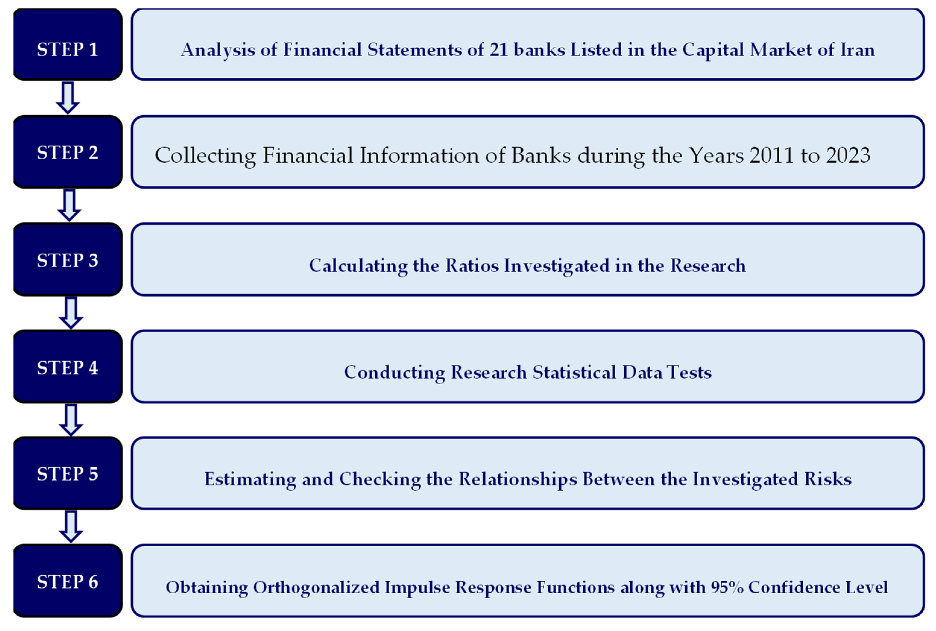
The information used in this research was extracted from the financial statements of 21 banks listed in the Iranian capital market during the years 2011 to 2023, and it was collected at a frequency of six months. Due to data availability limitations, this study primarily relies on semi-annual financial statements.

The statistical population includes all banks listed on the Tehran Stock Exchange (TSE) and Iran Fara Bourse (IFB) during the period 2011–2023. From this population, a sample of 21 banks was selected based on data availability, continuity in reporting, and completeness of financial disclosures across the 13-year horizon. Banks with missing or inconsistent data in key variables were excluded to ensure robustness.

The primary sources from which data were collected include, Codal.ir for audited financial statements (Equity, Loan portfolio, Cash balances, etc.), Central Bank of Iran for macroeconomic variables (GDP growth, CPI inflation, volatility index), and the TSETMC and TSE databases to cross-check institutional information.

To ensure the validity and reliability of the data, cross-verification was done across sources, and semi-annual aggregation was applied consistently to reduce seasonality effects. Only publicly disclosed, regulated, and audited figures were included.

As it is mentioned, the dataset of variables is extracted three main sources: banks’ financial statements, a comprehensive corporate database, and the databases of the Central Bank of Iran. The financial statements of the examined banks form the basis for calculating solvency, credit risk, and liquidity risk. These financial indicators are necessary to understand the stability and risk characteristics of the banking system. Also, the primary data for the variables were prepared from the comprehensive database of all companies listed on the Codal site, and the financial statements were derived from this data source. Finally, to represent the macroeconomic elements relevant to a banking risk assessment, data on key variables such as economic growth, inflation, and uncertainty measures were obtained from publicly available databases provided by the Central Bank of Iran. Figure 1 shows a schematic of the proposed method in this research.

The key variables of this research are solvency, credit risk, and liquidity risk. The equity ratio acts as an endogenous variable that approximates the bank’s solvency. This ratio provides a good insight into the bank’s ability to meet its obligations and absorb losses. Also, the ratio of non-performing loans to total loans is used as a proxy for the bank’s credit risk. This variable highlights the quality of the bank’s loan portfolio and reflects possible losses due to default. Finally, it is very important to mention that the ratio of cash to total assets is used as an indicator of liquidity risk, and a higher ratio indicates a lower liquidity risk, reflecting the bank’s capacity to fulfill short-term obligations (Dang, 2019).

In addition to endogenous variables, this research also introduces several exogenous variables to reduce the effects of omitted variables. The first variable is the economic growth parameter, measured by nominal GDP growth, which serves as a proxy for economic development due to its effect on the dynamics of the banking system. The second variable is the inflation measured by the growth rate of the Consumer Price Index (CPI), which captures inflationary pressures that affect bank operations and risk exposure. The third and final variable is the uncertainty index, which captures fluctuations in the economic environment and provides insights into risk implications for banks. In

Table 2. Variable Description and Sources.

Variable	Variable Name	Description	Mean	Std.	Min	Max	Source
SER	Shareholders’ Equity	Equity to Assets	−2.9%	38.1%	−303%	43.5%	Codal
CR	Credit Risk	Non-performing Loans Ratio	19.9%	27.1%	0.0%	201%	Codal
LR	Liquidity Risk	Cash to Assets	8.1%	8.8%	0.0%	100%	Codal
GRW	Economic Growth	Nom. GDP Growth	13.8%	9.9%	−2.1%	35.1%	CBI
INF	Inflation	CPI Growth	14.0%	9%	2.0%	33.0%	CBI
VIX	Volatility Index	Volatility Index	0.74	1.7	−3.16	5.83	CBI

, the description and sources of the variables used in this research are detailed.

Examining the complex relationship between solvency, credit risk, and liquidity risk necessitates the adoption of a comprehensive analytical framework. The conducted study emphasizes the applicability and flexibility of the Panel Vector Autoregression (VAR) model. It should be noted that the VAR model is designed to analyze the complex network of relationships between endogenous variables. The VAR model acts as a powerful analytical tool that enables us to detect and interpret time-dependent relationships in a system. By reconciling the relationships between different elements, this approach provides a comprehensive view to understand the evolving dynamics among solvency, credit risk, and liquidity risk.

The complexity of modern financial systems requires an analytical tool that can evaluate dynamic, time-varying interactions. VAR models, which have been noted for their ability to consider temporal and cross-sectional dimensions, are very efficient in revealing the internal relationships between these key indicators. One of the strengths of the VAR model is its ability to identify temporal interactions among endogenous variables, which is essential to describe and understand the sequential relationships that evolve over time. In this study, solvency, credit risk, and liquidity risk are treated as endogenous variables, while economic growth and inflation are included as exogenous factors to facilitate a broader understanding of systemic financial dynamics.

The advent of the Panel VAR (PVAR) method, pioneered by Holtz-Eakin et al. (1988) and developed as an extension of Sims’ traditional VAR model (Sims, 1980), revolutionized financial analysis by treating all variables within a system as endogenous. This approach allows for a comprehensive exploration of intricate relationships across multiple dimensions and time periods. The general formulation of PVAR is expressed as follows:

Y_it = A₀ + A₁Y_it−1 + A₂Y_it−2 + … + A_jY_it−j + BX_it + a_i + ε_it

(1)

This model encapsulates a vector Y_it comprising endogenous variables—solvency (SER), credit risk (CR), and liquidity risk (LR). Notably, PVAR accommodates a range of lag periods, offering insight into how past occurrences influence current financial dynamics.

The vector X_it consists of exogenous variables—economic growth (GRW), inflation (INF), and the volatility index (VIX). These macroeconomic variables play a pivotal role in understanding the broader contextual influences shaping financial outcomes.

Within this framework, there are N banks indexed i = 1, 2, …, 21 and time t = 1, 2, …, 11. The inclusion of lagged variables in the Panel Vector Autoregression (PVAR) model allows us to trace the historical influence of each variable. These lags, or lagged components, delineate how past values of exogenous variables affect the present state of the system. This temporal dimension unveils the intricate interplay between past occurrences and current conditions, unveiling the system’s temporal dynamics. Moreover, a_i within the PVAR architecture constitutes a vector encapsulating constants or unchanging attributes specific to individual banks.

Lastly, the term ε_it denotes the error term in the PVAR framework. This term captures the residual variability within the system that persists even after considering and accounting for the specified relationships among the variables. ε_it represents unexplained fluctuations or deviations that are not directly attributable to the defined interactions, highlighting the complexity inherent in the system under analysis.

To ensure the suitability of our variables for analysis, stationarity tests were conducted, affirming their stability without employing differencing techniques. The utilization of the Levin–Lin–Chu test (Levin et al., 2002) serves as a robust tool to validate the stationarity of our variables.

It should be mentioned that different models have been analyzed in different researches, but in this research, Equation (1) has been used to achieve the goal of the research. In past researches, PVECM model has been used as follows. The results obtained from the cointegration test show that all the variables of the model presented in Equations (2)–(4) are endogenous, while in certain cases some variables can be considered exogenous (Nkalu et al., 2020).

$$y_{it}={\beta }_i+A_{i1}{y}_{it-1}+\cdots +A_{ip}{y}_{it-p}+B_{i1}{y}_{-i.t-1}+\cdots +B_{ip}{y}_{-i.t-p}+{\epsilon }_{it}$$

(2)

where ${\beta }_i$ is an M-dimensional intercept vector and $A_{ij}$ (j = 1, …, p) refers to a set of M × N-dimensional coefficient matrices related to P lags of $y_{it}$. The effect of other economies’ lagged endogenous variables $y_{-i.t-p}$ is quantified via the matrices $B_{ij}$ with dimension M × (N − 1)M, while ${\epsilon }_{it}~N(0_{\mathrm{M}}.{\epsilon }_{it})$ is a Gaussian vector error term process with covariance matrix ${\sum }_{it}$. Equation (2) can be transformed into a conventional estimation equation as follows:

$$y_{it}=C_i{x}_{it}+B_i{x}_{-i.t}+{\epsilon }_{it}$$

(3)

The $y_{it}$ in Equation (3) can be expressed more compactly as a PVECM model as follows:

$$∆y_{it}={\beta }_0+\sum _{i=1}^n{\beta }_1∆y_{i.t}+\sum _{i=1}^k{\beta }_2∆X_{i.t}+{\beta }_3∆Z_{i.t-1}+{\epsilon }_{it}$$

(4)

The reported results from the panel unit root tests provide insightful statistics that affirm the stationary nature of the variables under investigation. The test statistics for solvency (SER), credit risk (CR), and liquidity risk (LR) yield noteworthy values of −2.68, −3.59, and −4.69, respectively. These statistics are accompanied by their corresponding probability values of 0.0037 ***, 0.0002 ***, and 0.0000 ***, respectively, indicating the statistical significance of the results.

Table 3. Panel Unit Root Test Results (*** indicate significance at the 1% levels).

Test		SER	CR	LR
Levin–Lin–Chu	Test Statistic	−2.68	−3.59	−4.69
	Prob.	0.0037 ***	0.0002 ***	0.0000 ***

shows the results of the Panel Unit Root test.

The corroborated stationarity of these variables, observed without employing differencing techniques, reinforces their suitability for inclusion in our model, facilitating a more accurate and reliable analysis of the dynamic relationships among the financial metrics studied.

Determining the optimal lag order is crucial in constructing a robust Panel Vector AutoRegression (VAR) model. The lag selection process, pivotal in capturing the temporal dependencies among variables, is conducted based on the Schwarz Information Criterion (SIC). The utilization of SIC helps identify the lag order that best balances model complexity and goodness of fit.

Table 4. VAR Lag Order Selection Criteria (*, **, and *** indicate significance at the 10%, 5%, and 1% levels).

Lag	LogL	LR	FPE	AIC	SC	HQ
0	286.0500	NA	2.60 × 10−5	−2.045150	−1.884359	−1.980568
1	1074.397	1535.512	7.74 × 10−8	−7.861173	−7.579790	−7.748156
2	1111.597	71.62388	6.27 × 10−8	−8.071621	−7.66964 *	−7.91016 *
3	1121.137	18.15500 *	6.24 × 10−8 *	−8.07565 *	−7.553084	−7.865764
4	1126.875	10.78967	6.40 × 10−8	−8.051304	−7.408143	−7.792980

presents the results of lag order selection, offering insights into the log-likelihood (LogL), likelihood ratio (LR), Final Prediction Error (FPE), Akaike Information Criterion (AIC), Schwarz Criterion (SC), and Hannan-Quinn Criterion (HQ) for various lag orders, ranging from 0 to 4.

The evaluation of these criteria unveils valuable information guiding the selection of an optimal lag order for our PVAR model. As indicated by the SC, the model complexity and fit balance favor the inclusion of lag 2*.

The consideration of Schwarz Information Criterion converges toward the selection of lag 2 as the most suitable order for our Panel VAR model. This choice strikes a balance between capturing the dynamic relationships among the variables while preventing overfitting, ensuring the reliability and accuracy of our subsequent analyses.

The Schwarz Information Criterion (SIC) provides several advantages compared to other criteria commonly used for lag order selection in VAR models. SIC strikes a balance between model complexity and goodness of fit. Unlike simpler criteria like AIC, SIC penalizes models more rigorously for increased complexity, which helps avoid overfitting and ensures a more robust model. SIC exhibits consistency, meaning that as the sample size increases, it consistently selects the correct lag order. It also holds asymptotic efficiency properties, providing reliable and accurate estimations of the lag order even with limited sample sizes. Moreover, SIC adjusts for small-sample biases more effectively than other criteria such as AIC or Hannan-Quinn, ensuring that the selected model maintains robustness and performs well with different sample sizes. By considering both the goodness of fit and the number of parameters in the model, SIC reduces the risk of overfitting the data. It discourages excessively complex models that may capture noise instead of true underlying relationships. Finally, SIC generally leads to more consistent and reliable lag order selection across different datasets and model specifications. It tends to provide a balanced and stable choice regardless of the specific characteristics of the dataset.

Table 4 summarizes the lag order selection process based on the Schwarz Information Criterion (SIC) within the Bayesian Panel Vector Autoregression (VAR) model. It assesses various lag lengths to determine an optimal balance between model complexity and explanatory power, crucial for robust modeling without overfitting. This overview presents log-likelihood values, likelihood ratios (LR), Final Prediction Error (FPE), Akaike Information Criterion (AIC), Schwarz Criterion (SC), and Hannan-Quinn (HQ) for each lag order candidate, aiding in the identification of the most fitting model configuration.

The Granger Causality Test is a statistical method used to explore the direction and strength of causal relationships between variables within a system. Developed by Clive Granger, this test determines whether past values of one variable can forecast another variable’s present values, implying a causal relationship between them (Granger, 1969). The Granger Causality Test helps in understanding temporal precedence and provides insights into the potential causal links between variables.

The Granger Causality Test for heterogeneous panel data models is specifically employed to assess causality within a panel dataset where the variables might have differing individual characteristics. This test accounts for potential heterogeneity among the variables in a panel setting, enabling the examination of causality across diverse units in the dataset. The Granger Causality Test results reveal a directional influence among the variables. Both CR (Credit Risk) and SER (Shareholders’ Equity Ratio) exert a significant impact on each other, as evidenced by associated p-values (both p < 0.01). However, LR (Liquidity Risk) does not exhibit a significant influence from CR or SER in this analysis, as indicated by non-significant Chi-squared values. The suggested sequential order of variables based on Granger causality is CR followed by SER and then LR.

Table 5. Results of Granger Causality Test for Heterogeneous Panel Data Models (*, **, and *** indicate significance at the 10%, 5%, and 1% levels).

Dep. Variable		SER	CR	LR
CR	Statistic	51.9		2.2
	Prob.	0.000 ***		0.31
SER	Statistic		3.57	7.0
	Prob.		0.16	0.03 **
LR	Statistic	1.07	0.45
	Prob.	0.58	0.79

shows the results of Granger Causality Test for Heterogeneous Panel Data Models. The null hypothesis states that the omitted variable does not cause the Granger dependent variable. Also, *, **, and *** indicate significance at the 10%, 5%, and 1% levels. It should be noted that the results of Granger Causality Test for Heterogeneous Panel Data Models are shown in Table 5.

The Johansen Cointegration Test (Johansen, 1991) was conducted to ascertain the existence of long-term relationships among the variables, which is critical for selecting an appropriate modeling technique between the Vector Autoregression (VAR) model and the Vector Error Correction Model (VECM). Upon evaluating the information criteria table, the selected model for testing cointegration includes an intercept but no trend component. This decision is based on the Schwarz Criteria, indicating that among the considered models, the one with an intercept and no trend yields the most suitable specifications for conducting the cointegration test. It should be mentioned that

Table 6. Various Information Criteria Scores for Different Models (* indicate significance at the 10% level).

Information Criteria by Rank and Model.
Data Trend:	None	None	Linear	Linear	Quadratic
Rank or	No Intercept	Intercept	Intercept	Intercept	Intercept
No. of CEs	No Trend	No Trend	No Trend	Trend	Trend
Schwarz Criteria by Rank (Rows) and Model (Columns)
0	−7.751723	−7.751723	−7.713348	−7.713348	−7.662647
1	−7.813046	−7.819743 *	−7.796889	−7.779522	−7.746283
2	−7.754417	−7.794424	−7.777091	−7.748327	−7.731789
3	−7.662338	−7.709185	−7.709185	−7.662963	−7.662963

shows Various Information Criteria Scores for Different Models.

The Trace and Maximum Eigenvalue tests play crucial roles in identifying the number of long-term relationships, also known as cointegrating relationships, among variables. These tests help ascertain the existence and quantify the number of stable, significant associations between variables over extended periods. The Trace test examines the total number of cointegrating relationships present in the system. Similarly, the Maximum Eigenvalue test focuses on identifying the maximum number of cointegrating relationships. Both tests utilize critical values to evaluate the significance of these relationships, aiding in the determination of the number of long-term connections among the variables. The analysis reveals the presence of two distinct cointegrating equations. These equations unveil the enduring associations among the variables CR, SER, and LR. Each equation outlines the normalized cointegrating coefficients and adjustment coefficients, providing insights into the relationships between these variables within each equation (MacKinnon, 1999). Additionally, the MacKinnon–Haug–Michelis p-values and the results of the Vector Error Correction estimation are presented in

Table 7. MacKinnon–Haug–Michelis p-Values (*, **, and *** indicate significance at the 10%, 5%, and 1% levels).

Unrestricted Cointegration Rank Test (Trace)
Hypothesized	Eigenvalue	Trace	0.05 Critical Value	Prob. **
No. of CE(s)		Statistic
None *	0.173386	107.7853	35.19275	0.0000
At most 1 *	0.092515	44.56665	20.26184	0.0000
At most 2 *	0.036476	12.33657	9.164546	0.0121
Unrestricted Cointegration Rank Test (Maximum Eigenvalue)
None *	0.173386	63.21865	22.29962	0.0000
At most 1 *	0.092515	32.23009	15.89210	0.0001
At most 2 *	0.036476	12.33657	9.164546	0.0121

and

Table 8. Vector Error Correction Estimation.

Vector Error Correction Estimates
Sample (Adjusted): 1391S1 1401S2
Included Observations: 332 After Adjustments
Standard Errors in ( ) and T-Statistics in [ ]
Cointegrating Eq.	CointEq.1
CR(-1)	1.000000
SER(-1)	0.448882
	(0.06378)
	[7.03814]
LR(-1)	−0.095031
	(0.28962)
	[−0.32812]
C	−0.196085
	(0.04171)
	[−4.70065]
Error Correction:	D(CR)	D(SER)	D(LR)
CointEq1	−0.340153	−0.056564	−0.000156
	(0.04781)	(0.01785)	(0.01631)
	[−7.11528]	[−3.16962]	[−0.00954]
D(CR(-1))	0.046750	0.011701	−0.004294
	(0.05697)	(0.02127)	(0.01943)
	[0.82064]	[0.55023]	[−0.22102]
D(SER(-1))	−0.468330	0.572159	−0.077887
	(0.12252)	(0.04574)	(0.04179)
	[−3.82245]	[ 12.5099]	[−1.86383]
D(LR(-1))	−0.224851	0.114413	−0.354238
	(0.15270)	(0.05700)	(0.05208)
	[−1.47253]	[2.00722]	[−6.80166]
GRW	−0.128859	−0.010881	−0.069417
	(0.10095)	(0.03769)	(0.03443)
	[−1.27640]	[−0.28874]	[−2.01600]
INF	0.014701	−0.008776	0.053450
	(0.11102)	(0.04144)	(0.03787)
	[0.13242]	[−0.21175]	[ 1.41154]
VIX	−0.000378	−0.000927	0.001186
	(0.00627)	(0.00234)	(0.00214)
	[−0.06033]	[−0.39579]	[ 0.55445]
R-Squared	0.172313	0.376515	0.146092
Adj. R-Squared	0.157032	0.365004	0.130328
Sum sq. Resids	5.233215	0.729244	0.608795
S.E. Equation	0.126894	0.047369	0.043281
F-Statistic	11.27671	32.71052	9.267181
Log likelihood	217.8305	544.9787	574.9463
Akaike AIC	−1.270063	−3.240836	−3.421363
Schwarz SC	−1.189835	−3.160607	−3.341134
Mean Dependent	−0.000684	−0.012367	0.000298
S.D. Dependent	0.138209	0.059444	0.046410
Determinant Resid Covariance (dof adj.)		6.50 × 10−8
Determinant Resid Covariance		6.10 × 10−8
Log likelihood		1344.518
Akaike Information Criterion		−7.948906
Schwarz Criterion		−7.662375
Number of Coefficients		25

, respectively.

The Vector Error Correction Model (VECM) serves as a robust framework for analyzing variable dynamics, particularly in scenarios where long-term relationships among variables are evident. VECM’s applicability in modeling relationships characterized by both short-term fluctuations and enduring equilibrium has been well-documented (Johansen, 1991). This model is adept at handling established long-term associations, as emphasized in the cointegration analysis (Engle & Granger, 1987).

Simultaneously, it captures short-term deviations from equilibrium through an error correction mechanism. This mechanism essentially characterizes the swiftness with which the system readjusts to its equilibrium state following a disturbance. Additionally, VECM allows for the exploration of dynamic interactions between variables, providing valuable insights into short-term adjustments after deviations from long-term relationships. Given the identified long-term relationships among the variables CR, SER, and LR, the VECM is considered more appropriate than the Panel Vector Autoregression (PVAR) model due to its capability to handle cointegrated series. Unlike PVAR, VECM explicitly models the adjustment process toward long-term equilibrium, making it the preferred model for studying variables with established cointegrating relationships.

4. Results

The exploration of dynamics among solvency, credit risk, and liquidity risk utilized a sophisticated Vector Error Correction Model (VECM) in this analysis. Spanning an extensive dataset across 12 years, encompassing 21 banks from 2011 to 2023, the VECM framework was constructed with three endogenous variables and three exogenous variables. Its lag order of 2, determined by the Schwarz Information Criterion (SIC), enabled a comprehensive understanding of temporal relationships. To unravel the complex interplay among these financial factors, the analysis ventured beyond mere estimation. Orthogonalized Impulse Response Functions (IRFs) and variance decomposition were meticulously computed post-VECM estimation (Figure 2). These tools were instrumental in discerning the nuanced impact of each variable over the temporal horizon, shedding light on short-term dynamics and long-term equilibrium relationships.

In configuring the model, the variable ordering, denoted as Yit = [CRit, SERit, LRit], was meticulously aligned with the Granger causality results, ensuring coherence and consistency. This ordering, following the Cholesky technique, strategically positioned SER as the most endogenous variable within the framework. Meanwhile, LR emerged as the most exogenous, reflecting its limited influence on the dynamics compared to other variables in the model. This deliberate arrangement contributes to a comprehensive understanding of the intricate relationships among these critical financial indicators.

The Impulse Response Function (IRF) technique is a robust analytical method used to examine the dynamic interactions among variables in a system over time. It illuminates the impact of a one-time shock or innovation to a particular variable on the entire system’s response, depicting how each variable reacts and influences others within the system. By computing IRFs, analysts gain valuable insights into short-term reactions and long-term equilibrium relationships among the variables.

The conducted IRF analysis revealed intriguing insights into the relationships among solvency, credit risk, and liquidity risk in the banking sector. A pivotal finding was the inverse relationship observed between a bank’s solvency and its credit risk. A solvent bank tended to exhibit lower credit risk, reflecting a certain level of financial robustness. However, the effect of solvency on credit risk became constant after five periods. On the other hand, solvency did not exhibit a substantial effect on liquidity risk. Moreover, the study indicated a positive impact of a favorable liquidity position on a bank’s solvency, aligning with anticipated expectations. In fact, the response to a positive shock in liquidity showcased a positive impact on the solvency variable, SER, indicating an increase in solvency over time. However, this liquidity-driven impact exhibited a relatively lower influence on credit risk. Conversely, a higher level of credit risk revealed a negative influence on a bank’s solvency, potentially leading to a decline in solvency over time. These findings underscore the intricate interplay among these pivotal financial variables within the banking sector, shedding light on their complex dynamics and mutual influence over time.

Variance decomposition is a powerful analytical tool used to discern the extent to which each variable contributes to the overall variability in a system over a specified time horizon. It disentangles the proportion of variability in each variable that can be attributed to its own past values (autoregressive component) and the influence from other variables within the system. By quantifying these contributions, variance decomposition aids in understanding the relative importance of each variable in explaining fluctuations within the system. In

Table 9. Variance Decomposition of Variables.

Period	S.E.	CR	SER	LR
Variance Decomposition of CR
1	0.126894	100.0000	0.000000	0.000000
2	0.161197	96.23614	3.502368	0.261490
3	0.180135	91.06805	8.654307	0.277638
4	0.193946	85.79814	13.90163	0.300228
5	0.205208	81.14106	18.55515	0.303796
6	0.214977	77.13455	22.56122	0.304231
7	0.223742	73.70028	25.99807	0.301649
8	0.231800	70.72830	28.97357	0.298130
9	0.239333	68.12795	31.57793	0.294124
10	0.246467	65.82818	33.88178	0.290038
Variance Decomposition of SER
1	0.047369	1.892068	98.10793	0.000000
2	0.088837	3.853944	95.81276	0.333297
3	0.127474	6.322745	93.23779	0.439464
4	0.163421	8.815383	90.64604	0.538579
5	0.196785	11.07934	88.31437	0.606285
6	0.227833	13.02877	86.31291	0.658315
7	0.256799	14.66442	84.63792	0.697656
8	0.283910	16.02135	83.25036	0.728290
9	0.309374	17.14385	82.10372	0.752428
10	0.333378	18.07424	81.15399	0.771770
Variance Decomposition of LR
1	0.043281	0.612912	1.527705	97.85938
2	0.051408	0.625126	1.084414	98.29046
3	0.060930	0.529512	0.772592	98.69790
4	0.068266	0.443168	0.646201	98.91063
5	0.075108	0.370005	0.570070	99.05993
6	0.081276	0.315993	0.531194	99.15281
7	0.087023	0.276654	0.508319	99.21503
8	0.092398	0.248407	0.495500	99.25609
9	0.097475	0.227909	0.488043	99.28405
10	0.102298	0.212814	0.483840	99.30335

presents the variance decomposition results for the variables used in this study.

Finally for each model variable we compute the variance decomposition. The results of the variance decomposition over a 12-year horizon following the initial shock are summarized in the Table 9. The variances of SER are influenced by the variable CR, with CR’s impact showing a progressive increase over time on SER. The variance of credit risk is partially explained by SER, while the effect of liquidity is not statistically significant. The variance in liquidity risk is not significantly explained by the other variables. Table 9 shows variance decomposition at the horizon of 12 years for the PVAR variables.

Diagnostic tests including residual autocorrelation, normality, and heteroskedasticity were performed to validate model assumptions. Additionally, robustness checks with varying lag orders and sub-sample analysis confirmed the consistency of the main findings.

The empirical results obtained from the VECM analysis provide several critical insights into the interplay between credit risk, liquidity risk, and solvency in Iranian banks. The negative relationship between credit risk and solvency reinforces the findings of studies such as Imbierowicz and Rauch (2014) and Oino (2021), which suggest that a higher level of non-performing loans erodes capital buffers and reduces financial stability. This is particularly important in the Iranian context, where credit risk is amplified by weak borrower assessment systems and prolonged economic instability.

In contrast, the positive impact of liquidity on solvency highlights the role of liquidity buffers as a protective shield during financial stress. This finding aligns with the Basel III framework and supports the notion that maintaining sufficient liquid assets helps banks absorb shocks and sustain operations, especially in volatile environments. However, the limited effect of credit risk on liquidity observed in this study contradicts several studies in mature markets, possibly due to the specific regulatory structure and centralized monetary system in Iran.

Another important implication of the findings is the weak influence of solvency and credit risk on liquidity risk, suggesting that liquidity in Iranian banks is less responsive to fundamental risks and more affected by external constraints such as monetary policy, sanctions, and capital controls. This divergence from international trends emphasizes the need for context-specific risk management frameworks in emerging economies.

Moreover, the variance decomposition analysis reveals that while solvency and credit risk mutually influence each other over time, liquidity risk remains mostly exogenous. This has practical implications for policy makers, indicating that improving bank liquidity may require broader financial reforms beyond internal risk mitigation strategies.

These findings contribute to the theoretical discourse on systemic risk by emphasizing the asymmetric and context-dependent nature of interactions among key banking risks. They also offer practical guidance to regulators, suggesting that credit quality and liquidity reserves should be managed together, but with distinct tools and priorities depending on the dominant macroeconomic risks in the environment.

While the empirical analysis in this study is limited by the availability of certain macroeconomic variables, it is essential to recognize that economic channels play a critical role in influencing the relationships between bank risk components such as liquidity risk, credit risk, and solvency risk. In particular, government fiscal conditions, such as budget deficits, can have direct and indirect effects on banks’ risk profiles. As outlined by Silva (2021), government deficits can increase credit risk through both direct channels, such as government guarantees, and indirect channels, such as multipliers, affecting banks’ exposure to non-performing loans (NPLs). Furthermore, deficits also influence banks’ liquidity via their effects on sovereign bonds and credit risk, impacting banks’ provisions, which are a significant expense accrual, ultimately affecting their profitability. This interplay suggests that government fiscal policies, including decisions on deficit financing, directly shape banks’ financial health and stability. The findings by Dantas et al. (2023) also support this view, indicating that government guarantees and earnings smoothing play significant roles in mitigating risks at the bank level.

Another critical economic channel, particularly relevant to the period of this study, is geopolitical uncertainty, with events like the Brexit referendum and the 2020 COVID-19 pandemic having substantial global spillover effects. The Brexit vote introduced significant uncertainty across both developed and emerging-market economies, including Iran’s, despite its relative economic disconnection from the U.S. (Campello et al. (2022)). Such geopolitical developments can impact corporate investment, labor markets, and financial stability, indirectly affecting bank risk-taking behaviors. Moreover, geopolitical uncertainty can increase volatility in both corporate earnings and sovereign debt markets, further influencing banks’ credit and liquidity risk exposure. Given the economic interconnectedness of global markets, including Iran’s, regional spillovers and macroeconomic shocks during the sample period likely influenced the dynamics of risk-taking behaviors within the banking sector.

5. Conclusions

This study investigates the dynamic interactions among credit risk, liquidity risk, and solvency in Iranian banks using a Panel Vector Error Correction Model (VECM) over the period 2011–2023. The results reveal a significant negative effect of credit risk on bank solvency, highlighting the vulnerability of capital adequacy to loan default exposure. In contrast, liquidity risk does not appear to significantly influence solvency or credit risk, suggesting its role is more isolated in the Iranian banking context. Meanwhile, higher solvency levels are shown to reduce credit risk, underscoring the importance of strong capital buffers.

Iran’s banking sector presents a unique case of systemic risk under persistent sanctions and inflationary pressure. Analyzing risk interactions in this environment not only adds to the literature on emerging markets but also demonstrates how banks operate under prolonged financial constraint, offering lessons for regions facing economic turbulence or institutional fragility.

In the Iranian banking system, liquidity constraints are primarily driven by funding liquidity shortages rather than market liquidity, due to the underdeveloped state of capital markets and limited asset tradability. As suggested by Brunnermeier and Pedersen (2009), market liquidity and funding liquidity are interconnected, but in Iran’s case, the dominance of government ownership and reliance on central bank facilities make funding liquidity the more relevant dimension. Therefore, the results should be interpreted within the framework of constrained funding access rather than impaired market liquidity.

Banks face significant exposure to various risks. The 2008 financial crisis highlighted the critical importance of bank risk management and its far-reaching economic consequences. From a national perspective, banking crises have historically led to severe economic disruptions, demonstrating the systemic vulnerability associated with financial institutions. In this study, we provide new empirical evidence about the relationship between bank risks and bank solvency. We show that a better liquidity position of a bank has a positive effect on a bank’s solvency, underlining the importance of liquidity management in the banking industry.

Moreover, our findings revealed an anticipated adverse impact of credit risk on a bank’s solvency. However, its influence on liquidity risk did not demonstrate statistical significance. This implies that a loan default significantly impacts a bank’s solvency compared to its effect on liquidity risk. In essence, efficient cash and liquidity management may not inherently translate to improved credit risk management. Additionally, a bank might not encounter liquidity issues even with a higher percentage of non-performing loans, but concurrently, this could compromise its solvency.

Regulatory guidelines often stipulate the maintenance of a certain solvency level to ensure financial stability. Meeting these requirements could be a priority for banks, directing their efforts toward bolstering solvency while not directly affecting liquidity management. Also, the quality of assets held by banks might be such that while non-performing loans increase credit risk, they may not directly affect the liquidity position. Banks may maintain sufficient liquid assets to address short-term obligations even in the presence of increased credit risk.

Finally, an increased solvency decreases a bank’s credit risk, but it does not impact its liquidity. Improved solvency implies a bolstered capital base. Banks with higher solvency ratios are better positioned to absorb losses from non-performing loans, thereby reducing their credit risk. However, this surplus capital does not directly affect liquidity, as it may be primarily reserved for credit risk coverage rather than short-term liquidity needs.

For prospective avenues of research, data envelopment analysis (DEA) models (Henriques et al., 2020; Peykani et al., 2020; Y. C. Chen et al., 2020; Peykani et al., 2022; Ben Lahouel et al., 2024) and machine learning (ML) algorithms (Bhatore et al., 2020; Petropoulos et al., 2020; Bussmann et al., 2021; Shetty et al., 2022; Shi et al., 2022; Araujo et al., 2023; Doumpos et al., 2023; Kumar et al., 2023; Usman et al., 2023; Zaki et al., 2024) could be employed to examine the interrelationships among solvency, liquidity, and credit risks in the banking system. Additionally, incorporating analyses of operational and market risks would further enrich the understanding of comprehensive bank risk dynamics.

This research contributes to the theoretical literature on systemic risk in emerging markets by demonstrating the asymmetric and directional nature of the relationships among key banking risks. It adds empirical support to Minsky’s Financial Instability Hypothesis and validates elements of Basel III’s integrated risk management framework, especially regarding the reinforcing feedback loop between credit risk and solvency. By using the VECM framework, the study emphasizes the necessity of modeling both short-term shocks and long-term equilibrium in the context of financial fragility.

From a policy perspective, the findings suggest that Iranian banks and regulators should prioritize strengthening capital adequacy as a proactive strategy to mitigate credit risk. While liquidity buffers remain important, they appear to play a secondary role in determining financial resilience in the current environment. Furthermore, regulators may consider implementing differentiated capital requirements based on the risk profiles of individual banks, especially those with high exposure to non-performing loans. Risk managers should also avoid assuming that liquidity improvements will automatically reduce credit risk and instead address the two dimensions through targeted and separate policies.

This study is subject to certain limitations. First, the reliability of bank-reported data in Iran may be affected by regulatory incentives or disclosure inconsistencies. Second, the generalization of the results to other emerging markets should be made cautiously, given the unique macro-financial context shaped by sanctions, inflation volatility, and centralized banking regulations.

Future studies could explore additional risk dimensions—such as operational risk and market risk—and their integration with the current framework. Moreover, Data Envelopment Analysis (DEA) and Machine Learning (ML) techniques can provide alternative, non-parametric insights into risk efficiency and prediction models. Cross-country comparisons could also help contextualize the Iranian case within broader global trends.

While this study incorporates VIX as a general proxy for market-based uncertainty, we acknowledge the limitations arising from the unavailability of more context-specific macroeconomic indicators—particularly those reflecting fiscal dynamics, regional geopolitical shocks, and broader global uncertainty spillovers. Due to data constraints and concerns about the consistency and reliability of such indicators for Iran and its key economic partners, we refrained from including them in our empirical model to preserve internal validity. Future research could benefit from the use of region-specific uncertainty indices and comprehensive macroeconomic datasets (e.g., from sources such as the Economic Policy Uncertainty Index), enabling a deeper exploration of the transmission mechanisms linking macro-level shocks to bank-level risk dynamics.

While the current study has focused on available data and highlighted the limitations of incorporating certain macroeconomic variables, we believe that future research could significantly benefit from the inclusion of broader fiscal and geopolitical data. Specifically, studies incorporating government deficit data and geopolitical events (such as trade wars, sanctions, or regional conflicts) would provide a more comprehensive understanding of the external shocks impacting banks’ risk profiles. Future analyses could also explore the potential influence of other economic conditions, such as GDP growth, inflation, and global market volatility, using more region-specific and high-quality datasets. These studies, ideally drawing from sources like Campello et al. (2022), Cortes et al. (2024), Silva (2021), Zaki et al. (2024), Campello et al. (2023), and Cortes et al. (2019), would offer deeper insights into the complex interdependencies between macroeconomic conditions and bank risks.

References

1. Abbas, F., Iqbal, S., & Aziz, B. (2019). The impact of bank capital, bank liquidity and credit risk on profitability in postcrisis period: A comparative study of US and Asia. Cogent Economics & Finance, 7(1), 1605683. [Google Scholar]
2. Abdelaziz, H., Rim, B., & Helmi, H. (2022). The interactional relationships between credit risk, liquidity risk and bank profitability in MENA region. Global Business Review, 23(3), 1–23. [Google Scholar] [CrossRef]
3. Adam, M., Soliman, A. M., & Mahtab, N. (2023). Measuring enterprise risk management implementation: A multifaceted approach for the banking sector. The Quarterly Review of Economics and Finance, 87, 244–256. [Google Scholar] [CrossRef]
4. Affandi, E., Ng, T. F., Pereira, J. J., Ahmad, F., & Banks, V. J. (2023). Revalidation technique on landslide susceptibility modelling: An approach to local level disaster risk management in Kuala Lumpur, Malaysia. Applied Science, 13(2), 768. [Google Scholar] [CrossRef]
5. Ahamed, F. (2021). Determinants of liquidity risk in the commercial banks in Bangladesh. European Journal of Business and Management Research, 6(1), 164–169. [Google Scholar] [CrossRef]
6. Aldasoro, I., Cho, C. H., & Park, K. (2022). Bank solvency risk and funding cost interactions: Evidence from Korea. Journal of Banking & Finance, 134, 106348. [Google Scholar]
7. Al-Husainy, N. M., & Jadah, H. M. (2021). The effect of liquidity risk and credit risk on the bank performance: Empirical evidence from Iraq. Journal of Economics, 3(1), 58–67. [Google Scholar] [CrossRef]
8. Anton, S. G., & Nucu, A. E. A. (2020). Enterprise risk management: A literature review and agenda for future research. Journal of Risk and Financial Management, 13(11), 281. [Google Scholar] [CrossRef]
9. Araujo, D., Bruno, G., Marcucci, J., Schmidt, R., & Tissot, B. (2023). Machine learning applications in central banking. Journal of AI, Robotics & Workplace Automation, 2(3), 271–293. [Google Scholar]
10. Arif, A., & Anees, A. N. (2012). Liquidity risk and performance of banking system. Journal of Financial Regulation and Compliance, 20(2), 182–195. [Google Scholar] [CrossRef]
11. Barongo, R. I., & Mbelwa, J. T. (2024). Using machine learning for detecting liquidity risk in banks. Machine Learning with Applications, 15, 100511. [Google Scholar] [CrossRef]
12. Basel Committee on Banking Supervision. (2010). Basel III: A global regulatory framework for more resilient banks and banking systems. Bank for International Settlements. Available online: https://www.bis.org/publ/bcbs189.pdf (accessed on 27 March 2025).
13. Bawa, J., & Basu, S. (2013). Restructuring assets reform, 2013: Impact of operational ability, liquidity, bank capital, profitability and capital on bank credit risk. IIMB Management Review, 32(3), 267–279. [Google Scholar] [CrossRef]
14. Ben Lahouel, B., Taleb, L., Ben Zaied, Y., & Managi, S. (2024). Financial stability, liquidity risk and income diversification: Evidence from European banks using the CAMELS–DEA approach. Annals of Operations Research, 334(1), 391–422. [Google Scholar] [CrossRef]
15. Berger, A. N., & Demirgüç-Kunt, A. (2021). Banking research in the time of COVID-19. Journal of Financial Stability, 57, 100939. [Google Scholar] [CrossRef]
16. Bhatore, S., Mohan, L., & Reddy, Y. R. (2020). Machine learning techniques for credit risk evaluation: A systematic literature review. Journal of Banking and Financial Technology, 4(1), 111–138. [Google Scholar] [CrossRef]
17. Bhimjee, D. C., Ramos, S. B., & Dias, J. G. (2016). Banking industry performance in the wake of the global financial crisis. International Review of Financial Analysis, 48, 376–387. [Google Scholar] [CrossRef]
18. Brei, M., Jacolin, L., & Noah, A. (2020). Credit risk and bank competition in sub-saharan Africa. Emerging Markets Review, 44, 100716. [Google Scholar] [CrossRef]
19. Breitenstein, M., Nguyen, D. K., & Walther, T. (2021). Environmental hazards and risk management in the financial sector: A systematic literature review. Journal of Economic Surveys, 35(2), 512–538. [Google Scholar] [CrossRef]
20. Brownlees, C., Hans, C., & Nualart, E. (2021). Bank credit risk networks: Evidence from the Eurozone. Journal of Monetary Economics, 117, 585–599. [Google Scholar] [CrossRef]
21. Brunnermeier, M. K., & Pedersen, L. H. (2009). Market liquidity and funding liquidity. The Review of Financial Studies, 22(6), 2201–2238. [Google Scholar] [CrossRef]
22. Bussmann, N., Giudici, P., Marinelli, D., & Papenbrock, J. (2021). Explainable machine learning in credit risk management. Computational Economics, 57(1), 203–216. [Google Scholar] [CrossRef]
23. Cafferata, A., Casellina, S., Landini, S., & Uberti, M. (2023). Financial fragility and credit risk: A simulation model. Communications in Nonlinear Science and Numerical Simulation, 116, 106879. [Google Scholar] [CrossRef]
24. Cahyandari, R., Kalfin, S., Purwani, S., Ratnasari, D., Herawati, T., & Mahdi, S. (2023). The development of sharia insurance and its future sustainability in risk management: A systematic literature review. Sustainability, 15(10), 8130. [Google Scholar] [CrossRef]
25. Campello, M., Cortes, G. S., d’Almeida, F., & Kankanhalli, G. (2022). Exporting UNCERTAINTY: The impact of brexit on corporate America. Journal of Financial and Quantitative Analysis, 57, 3178–3222. [Google Scholar] [CrossRef]
26. Campello, M., Kankanhalli, G., & Muthukrishnan, P. (2023). Corporate hiring under COVID-19: Financial constraints and the nature of new jobs. Journal of Financial and Quantitative Analysis, 59, 1541–1585. [Google Scholar] [CrossRef]
27. Chen, Y., Shen, C., Kao, L., & Yeh, C. (2018). Bank liquidity risk and performance. Review of Pacific Basin Financial Markets and Policies, 21(1), 1850007. [Google Scholar] [CrossRef]
28. Chen, Y. C., Chiu, Y. H., & Chiu, C. J. (2020). The performance evaluation of banks considering risk: An application of undesirable relation network DEA. International Transactions in Operational Research, 27(2), 1101–1120. [Google Scholar] [CrossRef]
29. Cheng, M., & Qu, Y. (2020). Does bank FinTech reduce credit risk? Evidence from China. Pacific-Basin Finance Journal, 63, 101398. [Google Scholar] [CrossRef]
30. Chenga, L., Nsiah, T. K., Charlesc, O., & Ayisid, A. L. (2020). Credit risk, operational risk, liquidity risk on profitability. A study on South Africa commercial banks: A PLS-SEM analysis. Revista Argentina de Clínica Psicológica, XXIX, 5–18. [Google Scholar] [CrossRef]
31. Choudhary, M. A., & Limodio, N. (2022). Liquidity risk and long-term Finance: Evidence from a natural experiment. The Review of Economic Studies, 89(3), 1278–1313. [Google Scholar] [CrossRef]
32. Cont, R., Kotlicki, A., & Valderrama, L. (2020). Liquidity at risk: Joint stress testing of solvency and liquidity. Journal of Banking & Finance, 118, 105871. [Google Scholar]
33. Cornwell, N., Bilson, C., Gepp, A., Stern, S., & Vanstone, B. J. (2023). Modernising operational risk management in financial institutions via data-driven causal factors analysis: A pre-registered report. Pacific-Basin Finance Journal, 77, 101906. [Google Scholar] [CrossRef]
34. Cortes, G. S., Silva, T. C., & van Doornik, B. F. N. (2019). Credit shock propagation in firm networks: Evidence from government bank credit expansions. Available online: https://www.bcb.gov.br/pec/wps/ingl/wps507.pdf (accessed on 12 May 2025).
35. Cortes, G. S., Vossmeyer, A., & Weidenmier, M. D. (2024). Stock volatility and the war puzzle: The military demand channel, NBER working paper 29837. National Bureau of Economic Research. [Google Scholar] [CrossRef]
36. Dang, V. D. (2019). The effects of loan growth on bank performance: Evidence from Vietnam. Management Science Letters, 9(6), 899–910. [Google Scholar] [CrossRef]
37. Dantas, M., Merkley, K. J., & Silva, F. B. G. (2023). Government guarantees and banks’ income smoothing. Journal of Financial Services Research, 63(2), 123–173. [Google Scholar] [CrossRef]
38. De Bandt, O., Lecarpentier, S., & Pouvelle, C. (2022). Determinants of banks’ liquidity: A French perspective on interactions between market and regulatory requirements. Journal of Banking & Finance, 124, 106032. [Google Scholar]
39. Ding, B. Y., & Wei, F. (2023). Overlapping membership between risk management committee and audit committee and bank risk-taking: Evidence from China. International Review of Financial Analysis, 86, 102501. [Google Scholar] [CrossRef]
40. Djebali, N., & Zaghdoudi, K. (2020). Threshold effects of liquidity risk and credit risk on bank stability in the MENA region. Journal of Policy Modeling, 42(5), 1049–1063. [Google Scholar] [CrossRef]
41. Doko, F., Kalajdziski, S., & Mishkovski, I. (2021). Credit risk model based on central bank credit registry data. Journal of Risk and Financial Management, 14(3), 138. [Google Scholar] [CrossRef]
42. Doumpos, M., Zopounidis, C., Gounopoulos, D., Platanakis, E., & Zhang, W. (2023). Operational research and artificial intelligence methods in banking. European Journal of Operational Research, 306(1), 1–16. [Google Scholar] [CrossRef]
43. Engle, R. F., & Granger, C. (1987). Co-integration and error correction: Representation, estimation, and testing. Econometrica: Journal of the Econometric Society, 55(2), 251–276. [Google Scholar] [CrossRef]
44. Fejza, F., Nace, D., & Kulla, O. (2022). The credit risk problem—A developing country case study. Risks, 10(8), 146. [Google Scholar] [CrossRef]
45. Galletta, S., Goodell, J. W., Mazzù, S., & Paltrinieri, A. (2023). Bank reputation and operational risk: The impact of ESG. Finance Research Letters, 51, 103494. [Google Scholar] [CrossRef]
46. Ghenimi, A., Chaibi, H., & Omri, M. A. B. (2017). The effects of liquidity risk and credit risk on bank stability: Evidence from the MENA region. Borsa Istanbul Review, 17(4), 238–248. [Google Scholar] [CrossRef]
47. Ghenimi, A., Chaibi, H., & Omri, M. A. B. (2021). Liquidity risk determinants: Islamic vs. conventional banks. International Journal of Law and Management, 63(1), 65–95. [Google Scholar] [CrossRef]
48. González, F. (2005). Bank regulation and risk-taking incentives: An international comparison of bank risk. Journal of Banking & Finance, 29(5), 1153–1184. [Google Scholar]
49. Granger, C. W. (1969). Investigating causal relations by econometric models and cross-spectral methods. Econometrica, 37(3), 424–438. [Google Scholar] [CrossRef]
50. Henriques, I. C., Sobreiro, V. A., Kimura, H., & Mariano, E. B. (2020). Two-stage DEA in banks: Terminological controversies and future directions. Expert Systems with Applications, 161, 113632. [Google Scholar] [CrossRef] [PubMed]
51. Holtz-Eakin, D. N., Newey, W., & Rosen, H. S. (1988). Estimating vector autoregressions with panel data. Econometrica, 56(6), 1371–1395. [Google Scholar] [CrossRef]
52. Hoque, H., Andriosopoulos, D., Andriosopoulos, K., & Douady, R. (2015). Bank regulation, risk and return: Evidence from the credit and sovereign debt crises. Journal of Banking & Finance, 50, 455–474. [Google Scholar]
53. Imbierowicz, B., & Rauch, C. H. (2014). The relationship between liquidity risk and credit risk in banks. Journal of Banking & Finance, 40, 242–256. [Google Scholar]
54. Johansen, S. (1991). Estimation and hypothesis testing of cointegration vectors in gaussian vector autoregressive models. Econometrica, 59(6), 1551–1580. [Google Scholar] [CrossRef]
55. Kabir, M. N., Worthington, A., & Gupta, R. (2015). Comparative credit risk in Islamic and conventional bank. Pacific-Basin Finance Journal, 34, 327–353. [Google Scholar] [CrossRef]
56. Kil, K., Ciukaj, R., & Chrzanowska, J. (2021). Scoring models and credit risk: The case of cooperative banks in Poland. Risks, 9(7), 132. [Google Scholar] [CrossRef]
57. Kirikkaleli, D., & Kayar, E. U. (2023). The effect of economic, financial and political stabilities on the banking sector: Cases of six balkan countries. Sustainability, 15(4), 3000. [Google Scholar] [CrossRef]
58. Kumar, R., Grover, N., Singh, R., Kathuria, S., Kumar, A., & Bansal, A. (2023, March 23–25). Imperative role of artificial intelligence and big data in finance and banking sector. International Conference on Sustainable Computing and Data Communication Systems (pp. 523–527), Erode, India. [Google Scholar]
59. Laeven, L., & Levine, R. (2009). Bank governance, regulation and risk taking. Journal of Financial Economics, 93(2), 259–275. [Google Scholar] [CrossRef]
60. Lang, Q., Ma, F., Mirza, N., & Umar, M. (2023). The interaction of climate risk and bank liquidity: An emerging market perspective for transitions to low carbon energy. Technological Forecasting and Social Change, 191, 122480. [Google Scholar] [CrossRef]
61. Levin, A., Lin, C., & Chu, C. J. (2002). Unit root tests in panel data: Asymptotic and finite-sample properties. Journal of Econometrics, 108(1), 1–24. [Google Scholar] [CrossRef]
62. Lin, J., & Han, L. (2021). Lattice clustering and its application in credit risk management of commercial banks. Procedia Computer Science, 183, 145–151. [Google Scholar] [CrossRef]
63. Lopez, J. A., & Saidenberg, M. R. (2000). Evaluating credit risk models. Journal of Banking & Finance, 24(1–2), 151–165. [Google Scholar]
64. MacKinnon, J. G. (1999). Numerical distribution functions of likelihood ratio tests for cointegration. Journal of Applied Econometrics, 14(5), 563–577. [Google Scholar] [CrossRef]
65. Mateev, M., Sahyouni, A., & Tariq, M. U. (2023). Bank regulation, ownership and risk taking behavior in the MENA region: Policy implications for banks in emerging economies. Review of Managerial Science, 17, 287–338. [Google Scholar] [CrossRef]
66. Matey, J. (2021). Bank liquidity risk and bank credit risk: Implication on bank stability in Ghana. International Journal of Scientific Research in Multidisciplinary Studies, 7(4), 01–09. [Google Scholar]
67. Minsky, H. P. (1975). The financial instability hypothesis: An interpretation of Keynes and an alternative to “standard theory”. Nebraska Journal of Economics and Business, 16, 5–16. [Google Scholar] [CrossRef]
68. Mirza, N., Rahat, B., Naqvi, B., & Rizvi, K. A. (2023). Impact of Covid-19 on corporate solvency and possible policy responses in the EU. The Quarterly Review of Economics and Finance, 87, 181–190. [Google Scholar] [CrossRef]
69. Misman, F. N., & Bhatti, M. I. (2020). The determinants of credit risk: An evidence from ASEAN and GCC Islamic banks. Journal of Risk and Financial Management, 13(5), 89. [Google Scholar] [CrossRef]
70. Mohammad, S., Asutay, M., Dixon, R., & Platonova, E. (2020). Liquidity risk exposure and its determinants in the banking sector: A comparative analysis between Islamic, conventional and hybrid banks. Journal of International Financial Markets, Institutions and Money, 66, 101196. [Google Scholar] [CrossRef]
71. Naili, M., & Lahrichi, Y. (2022). Banks’ credit risk, systematic determinants and specific factors: Recent evidence from emerging markets. Heliyon, 8(2), e08960. [Google Scholar] [CrossRef]
72. Nkalu, C. N., Ugwu, S. C., Asogwa, F., & Kuma, P. (2020). Financial development and energy consumption in sub-Saharan Africa: Evidence from panel vector error correction modelriginal research. SAGE Open, 1–12. [Google Scholar] [CrossRef]
73. Noriega, J. P., Rivera, L. A., & Herrera, J. A. (2023). Machine learning for credit risk prediction: A systematic literature review. Data, 8(11), 169. [Google Scholar] [CrossRef]
74. Oino, I. (2021). Bank solvency: The role of credit and liquidity risks, regulatory capital and economic stability. Banks and Bank Systems, 16(4), 84–100. [Google Scholar] [CrossRef]
75. Park, S. R., & Jang, J. Y. (2021). The impact of ESG management on investment Decision: Institutional investors’ perceptions of country-specific ESG Criteria. International Journal of Financial Studies, 9(3), 48. [Google Scholar] [CrossRef]
76. Petropoulos, A., Siakoulis, V., Stavroulakis, E., & Vlachogiannakis, N. E. (2020). Predicting bank insolvencies using machine learning techniques. International Journal of Forecasting, 36(3), 1092–1113. [Google Scholar] [CrossRef]
77. Peykani, P., Hosseinzadeh Lotfi, F., Sadjadi, S. J., Ebrahimnejad, A., & Mohammadi, E. (2022). Fuzzy chance-constrained data envelopment analysis: A structured literature review, current trends, and future directions. Fuzzy Optimization and Decision Making, 21, 197–261. [Google Scholar] [CrossRef]
78. Peykani, P., Mohammadi, E., Farzipoor Saen, R., Sadjadi, S. J., & Rostamy-Malkhalifeh, M. (2020). Data envelopment analysis and robust optimization: A review. Expert Systems, 37, e12534. [Google Scholar] [CrossRef]
79. Peykani, P., Sargolzaei, M., Botshekan, M. H., Oprean-Stan, C., & Takaloo, A. (2023a). Optimization of asset and liability management of banks with minimum possible changes. Mathematics, 11(12), 2761. [Google Scholar] [CrossRef]
80. Peykani, P., Sargolzaei, M., Takaloo, A., & Sanadgol, N. (2023b). Investigating the monetary policy risk channel based on the dynamic stochastic general equilibrium model: Empirical evidence from Iran. PLoS ONE, 18(10), e0291934. [Google Scholar] [CrossRef]
81. Pozo, J., & Rojas, Y. (2023). Bank competition and credit risk: The case of Peru. Journal of Financial Stability, 66, 101119. [Google Scholar] [CrossRef]
82. Rezvani, S. M., Falcão, M. J., Komljenovic, D., & De Almeida, N. M. (2023). A systematic literature review on urban resilience enabled with asset and disaster risk management approaches and GIS-based decision support tools. Applied Science, 13(4), 2223. [Google Scholar] [CrossRef]
83. Sakouvogui, K. (2020). Impact of liquidity and solvency risk factors on variations in efficiency of US banks. Managerial Finance, 46(7), 883–895. [Google Scholar] [CrossRef]
84. Sharma, P., Mishra, B. B., & Rohatgi, S. K. (2023). Revisiting the impact of NPAs on profitability, liquidity and solvency: Indian banking system. IMIB Journal of Innovation and Management, 1(2), 167–180. [Google Scholar] [CrossRef]
85. Shetty, S., Musa, M., & Brédart, X. (2022). Bankruptcy prediction using machine learning techniques. Journal of Risk and Financial Management, 15(1), 35. [Google Scholar] [CrossRef]
86. Shi, S., Tse, R., Luo, W., D’Addona, S., & Pau, G. (2022). Machine learning-driven credit risk: A systemic review. Neural Computing and Applications, 34(17), 14327–14339. [Google Scholar] [CrossRef]
87. Sidhu, A. V., Abraham, R., Bhimavarapu, V. M., Kanoujiya, J., & Rastogi, S. (2023). Impact of liquidity on the efficiency of banks in india using panel data analysis. Journal of Risk and Financial Management, 16(9), 390. [Google Scholar] [CrossRef]
88. Silva, F. B. G. (2021). Fiscal deficits, bank credit risk, and loan-loss provisions. Journal of Financial and Quantitative Analysis, 56(5), 1537–1589. [Google Scholar] [CrossRef]
89. Sims, C. A. (1980). Macroeconomics and Reality. Econometrica, 48(1), 1–48. [Google Scholar] [CrossRef]
90. Telg, S., Dubinova, A., & Lucas, A. (2023). COVID-19, credit risk management modeling, and government support. Journal of Banking & Finance, 147, 106638. [Google Scholar]
91. Trang, L., Nhan, D., Hao, N., & Wong, W. (2021). Does bank liquidity risk lead to bank’s operational efficiency? A study in Vietnam. Advances in Decision Sciences, 25(4), 46–88. [Google Scholar]
92. Umar, M., Ji, X., Mirza, N., & Naqvi, B. (2021). Carbon neutrality, bank lending, and credit risk: Evidence from the Eurozone. Journal of Environmental Management, 296, 113156. [Google Scholar] [CrossRef]
93. Usman, T. M., Saheed, Y. K., Nsang, A., Ajibesin, A., & Rakshit, S. (2023). A systematic literature review of machine learning based risk prediction models for diabetic retinopathy progression. Artificial Intelligence in Medicine, 143, 102617. [Google Scholar] [CrossRef]
94. Varma, P., Nijjer, S., Sood, K., Grima, S., & Rupeika-Apoga, R. (2022). Thematic analysis of financial technology (Fintech) influence on the banking industry. Risks, 10(10), 186. [Google Scholar] [CrossRef]
95. Von Tamakloe, B., Boateng, A., Mensah, E. T., & Maposa, D. (2023). Impact of risk management on the performance of commercial banks in Ghana: A panel regression approach. Journal of Risk and Financial Management, 16(7), 322. [Google Scholar] [CrossRef]
96. Vuong, G., Thanh, P., Nguyen, C. X., Nguyen, D. M., & Duong, K. D. (2023). Liquidity creation and bank risk-taking: Evidence from a transition market. Heliyon, 9(9), e19141. [Google Scholar] [CrossRef]
97. Wang, J., Zhao, L., & Huchzermeier, A. (2021). Operations-finance interface in risk management: Research evolution and opportunities. Production and Operations Management, 30(2), 355–389. [Google Scholar] [CrossRef]
98. Wang, Y., Zhang, Y., Lu, Y., & Yu, X. (2020). A comparative assessment of credit risk model based on machine learning—A case study of bank loan data. Procedia Computer Science, 174, 141–149. [Google Scholar] [CrossRef]
99. Yanenkova, I., Nehoda, Y., Drobyazko, S., Zavhorodnii, A., & Berezovska, L. (2021). Modeling of bank credit risk management using the cost risk model. Journal of Risk and Financial Management, 14(5), 211. [Google Scholar] [CrossRef]
100. Zaki, A. M., Khodadadi, N., Lim, W. H., & Towfek, S. K. (2024). Predictive analytics and machine learning in direct marketing for anticipating bank term deposit subscriptions. American Journal of Business and Operations Research, 11(1), 79–88. [Google Scholar] [CrossRef]
101. Zhang, X., Zhang, X., Lee, C., & Zhao, Y. (2023). Measurement and prediction of systemic risk in China’s banking industry. Research in International Business and Finance, 64, 101874. [Google Scholar] [CrossRef]
Figure 1. The Schematic Summary of All Steps in the Proposed VECM.
Economies 13 00139 g001
Figure 2. Orthogonalized Impulse Response Functions along with 95% Confidence Level.
Economies 13 00139 g002