Abstract
The COVID-19 pandemic potentially affected stock prices in two non-mutually exclusive ways: discount rates and cash flows. This paper focuses on the latter and analyzes it through the lens of an asset-pricing model. It shows how workplace resilience and financial resilience interacted and significantly affected asset prices. The model-based equity premium increases with the probability of a disaster. The results suggest the significant amplification of workplace resilience by financial resilience. Specifically, the dividend growth of low-resilience firms is significantly more responsive to workplace flexibility and suffers more severely than that of high-resilience firms.
1. Introduction
COVID-19 has profoundly affected the economy and induced tremendous uncertainty in the financial markets. Governments adopted different types of social distancing policies to control the spread, especially in the first wave and the fever period of COVID (February to April 2020). These social distancing rules and lockdowns effectively influenced the working environment and firms’ performance (Koren & Pető, 2020, among others). The fast-growing literature asserts that firms with fewer labor constraints in the lockdown-restricted situation featured better performance (Bretscher et al., 2020), as firms with more flexibility in their workforce are expected to be less financially vulnerable in such situations, since they are less likely to face additional costs due to lockdowns and social distancing rules. Koren and Pető (2020) propose different dimensions of the firms’ workplace flexibility that played an important role in their cost of production, as well as the fluctuations in asset prices in response to the COVID-19 shock (Pagano et al., 2023).
In theory, COVID-19 can affect stock prices through two non-mutually independent channels: discount rates and cash flows. Pagano et al. (2023) focus mainly on the impact of the increase in perceived risk on expected excess returns (first channel). Back to the story of COVID, industries saw massive business disruption due to social distancing and lockdowns as a consequence of the pandemic, which affected the cost of production and especially the output of firms with less flexibility in their workplace. In such a turbulent market, conservative investors primarily focus on the price of an equity claim to the output of such firms as risky assets—that is, the expected future cash flows. Daadmehr (2024) shows that risks related to the working environment of a company, including the impact of the communication mode, teamwork, and physical presence, to which a company is exposed, can create heterogeneity in expected cash flows. According to Stulz (2025), managing such risks as consequences of the COVID pandemic crisis can potentially affect the value of firms. This paper concentrates on the second channel and, in a novel work, quantifies expected cash flows not just to fill the gap in the risk management literature, but to show how the impact of COVID-19 and corporate resilience can carry over from cash flows to expected returns. The characterization of resilience heterogeneity in expected cash flow sheds light on how this paper bridges a gap and links the real part of the economy, where the exogenous COVID-19 shock originated, to the financial market.
This paper analyzes the asset-pricing implications of the COVID-19 crisis, including its impact on the economy and firms’ production costs, in the context of a model with (i) a fictitious representative investor with Epstein–Zin–Weil preferences, who may prefer an early resolution of uncertainty in disasters1; and (ii) an exogenous dividend stream sensitive to the consequences of the COVID-19 disaster and to its contractionary effects on the real part of the economy. This study considers the cross-sectional time-varying impact of COVID-19 on the dividend stream as the interaction of two components: the cross-sectional firm-level impact of workplace resilience and the time-varying impact of aggregate economic contraction, as a control for the macro time effect of COVID-19. Specifically, it shows that the dividend growth of low-workplace-resilience firms is significantly more sensitive to workplace resilience and suffers more severely than that of high-workplace-resilience firms.
However, the impact of corporate financials was quite complex during the COVID-19 outbreak. Firms started raising capital just because of cash flow dry-up fears or to strengthen their ability to overcome difficulties during the first wave. Meanwhile, the provided credit, especially in small firms, could affect the capital structure and increase leverage. Consequently, the financial characteristics of firms, such as capital structure and liquidity, also played an important role in the performance of firms and were considerably influenced by a wide range of policies adopted in response to COVID-19, from corporate policies to public policies, including bank-loan guarantees and additional mitigation packages, for example, the Paycheck Protection Program, PPP loans (Fahlenbrach et al., 2020; Pagano & Zechner, 2022). This suggests that these characteristics may have also contributed to amplifying the degree of corporate resilience and, as a result, the response of asset prices (Daadmehr, 2024).
Some recent articles have shed light on the impact of corporate financial amplification on asset prices during COVID-19 period (Daadmehr, 2024; Ramelli & Wagner, 2020) and have found significant heterogeneity in resilience in expected returns by introducing a new “composite financial resilience” index that contains both workplace flexibility and “financial-based resilience” (Daadmehr, 2024). The novelty of this paper lies in the fact that it provides a simple example as evidence of the amplification effect and shows that cross-sectional and time-varying corporate financials can potentially amplify the overall effect of exogenous consequences of COVID-19, consistent with the evidence that better-financed firms before and during COVID-19 can better overcome the side effects of lockdown and the associated mitigation of COVID restrictions (Daadmehr, 2024; Fahlenbrach et al., 2020). Then, it quantifies “financial resilience” to capture the footprints of the impact of a wide range of different policies on the financial status of firms.
This paper proposes a new asset-pricing model with COVID-19 disaster embedding workplace resilience and financial resilience to investigate and track the impact of firms’ characteristics on asset-pricing implications. The novelty of this paper is directly related to how it quantifies the consequences of the exogenous COVID-19 crisis on the dividend stream that affects asset prices depending on the resilience of these two types of firms. In other words, it clarifies how resilience practically contributes to asset pricing and characterizes the resilience-heterogeneous equity premium by providing tractable formulas, showing that it increases with the probability of a disaster.
In line with Daadmehr (2024), this article shows that the effect of financial resilience of firms significantly amplifies the impact of workplace resilience and aggregate economic contraction due to COVID-19. The novel proposed an exogenous dividend stream, and its estimation provides an opportunity to compare the impact of firms’ financial resilience and workplace resilience. Meanwhile, estimated dividend growth highlights that the heterogeneous effect of workplace resilience is dominant, although the impact of firms’ financial resilience is statistically significant, demonstrating the need for characterization of “financial resilience”. The novel application of Dynamic Functional Principal Component Analysis (DFPCA) enables us to distinguish not only the main time-varying elements of financial resilience but also those that create significant cross-sectional variation. Finally, this paper empirically proves that valuation, liquidity, and solvency ratios play key roles in firms’ financial resilience and the corresponding amplification of workplace resilience. The results of this part shed light on possible corporate policies.
The paper is structured as follows. Section 2 clarifies how this paper contributes to the literature and postpones the introduction of resilience intuitions to Section 3. The model of the economy and the assumptions about the exogenous dividend stream at the firm level are presented in Section 4. The solution of the model appears in Section 5, where the closed form of the resilience-heterogeneous equity premium is presented. The results on both the effect of the macroeconomic contraction of COVID-19 and the estimated dividend stream are included in Section 6. The paper proposes the main components of financial resilience in Section 7 and then concludes.
2. Contribution to Literature
As the main novelty of this paper is to investigate resilience heterogeneity in expected cash flows and its role in asset pricing, this paper contributes to two main strands of literature: (i) corporate resilience and the impact of COVID-19 on the cross-section of stock returns, and (ii) asset pricing models with rare events.
On the one hand, this article attempts to discuss the impact of workplace resilience and financial resilience as an overall indicator of firms’ financial status. Since the emergence of COVID-19, many studies have started to explain the flexibility of firms or industries in such a pandemic crisis, specifically in response to health mitigation policies, social distancing rules, and lockdowns (among all Dingel & Neiman, 2020; Hensvik et al., 2020; Koren & Pető, 2020). This paper contributes to these studies more from the perspective of asset pricing than from corporate resilience and considers workplace resilience in the spirit of Koren and Pető (2020). As a key feature, this paper uses the data on workplace resilience and explains how and to what extent it significantly contributes to the asset-pricing model during the COVID pandemic.
Meanwhile, this paper takes into account financial resilience, as the fast-growing literature has already emphasized the importance of corporate financials on asset prices in response to a wide range of public and corporate policies (Ding et al., 2021; Fahlenbrach et al., 2020; Pagano & Zechner, 2022; Ramelli & Wagner, 2020). Daadmehr (2024) compares these two intuitions of resilience and provides a measure of corporate resilience, called the composite-financial resilience index, applicable in times of pandemics. This cross-sectional measure allows for the categorization of assets into more risky and less risky groups and enables investors to manage their resources. She provides different evidence of resilience heterogeneity in expected returns and expected future cash flows that can potentially originate from workplace resilience and financial resilience as an additional source of variation. This paper deviates from Daadmehr (2024) and quantifies the cross-sectional “time-varying” financial resilience, although the aim is not to propose an index. Contrary to the major part of these studies in corporate finance, this paper proposes a mechanism to estimate a mixed specification for exogenous dividend stream as an expected future cash flow. Since there is no empirical study on the link between these two types of resilience, nor theoretical work or background, this paper (Section 3.2) starts with simple empirical evidence to motivate the characterization of the exogenous dividend stream as a bridge between these two types of resilience.
According to the literature, it is noteworthy to mention and clarify the impact of the possibility of disaster on the macro time effect of the exogenous COVID-19 pandemic as the third source of variation. Among all, Gourio (2012), Gabaix (2012), and Wachter (2013) declare the time-varying probability of disaster that generates covariation in the equity premium. Ghaderi et al. (2022) develop the literature and consider the gradual unfolding disasters. They explain that investors are not aware of the true state of the economy and introduce a Bayesian learning framework showing that updating investors’ beliefs captures the effect of slowly unfolding disasters, as prices truly react to the consumption decline. They show that updating the agent’s belief accords with the true state of the economy. This paper deviates from Ghaderi et al. (2022) by considering disaster states as bad times of the economy. It empirically proves that COVID-19 has a tremendous impact on the economy and captures the impact of disaster and controls the time variation of expected cash flows for macroeconomic sensitivity to COVID-19 using the Markov-Switching approach. As opposed to Wachter and Zhu (2024) who use the jump Poisson process to capture the low and high intensity of disaster that defines disaster states based on two high and low amounts of disaster intensity, and apply a Markov-Switching simulation to investigate the impact of learning in asset pricing of rare disasters, this study considers disaster states as the bad times of the economy and “estimates” the probability of disaster, states, and the duration of regimes based on monthly GDP.
From an asset pricing perspective, this paper uses the general framework proposed by Barro (2006) but with a special case of EZ preferences. Contrary to Barro (2006), who proposes economic contraction due to rare events as a “random variable” and calibrates it, this article considers it as a “stochastic process” and provides an estimate for each month, using the Markov-Switching approach. The empirical analysis on this part shows that dividend growth was significantly sensitive to the overall economic contraction due to the COVID-19 phenomenon, with a conditional probability of 2 percent, in line with Barro (2006), who calibrates the disaster probability parameter. Another main difference is directly related to the idea of resilience.
“Resilience” in Asset Pricing:
In the asset pricing literature, many studies introduce resilience in the rare-disaster framework. Gabaix (2012) considers a deterministic aggregate consumption growth in the absence of disaster; however, consumption growth is magnified by a positive macroeconomic recovery rate when a disaster occurs. He presents an asset-specific dividend process magnified by a positive rate of surviving in a disaster period. The definition of time-varying “resilience” in his paper is an increasing function of the asset-specific survival rate. In the framework he proposed, resilience is a linearity-generating process that sees shock, uncorrelated with disaster occurrence. Since the definition of resilience highly depends on the type of disaster, this article, in contrast to Gabaix (2012), considers cross-sectional workplace resilience due to the natural feature of the COVID-19 pandemic and its effect on the workforce and firm costs through social distancing rules and lockdowns (similar to Daadmehr, 2024; Pagano et al., 2023).
This paper deviates from Pagano et al. (2023) in two aspects: First, it uses data on workplace resilience (in the spirit of Koren & Pető, 2020) rather than considering it as a parameter in the model. Moreover, this study considers workplace resilience, affecting the dividend stream cross-sectionally, and quantifies the cross-sectional time-varying impact of corporate financials as an additional part called financial resilience. Second, it provides monthly estimates for disaster probability rather than theoretical intuition for the probability of disaster as a parameter in the model. It should also be noted that this paper provides an empirical test as a prerequisite to having a particular definition of disaster state and the corresponding probabilities based on the intrinsic characteristic of COVID-19 and the Poisson distribution, as theoretically proposed by Daadmehr (2025). The striking difference is directly related to the role of the estimated Markov switching process as a control for the macro time effect of COVID-19, a necessary part as Barro (2006) declares.
This paper demonstrates the dominant heterogeneous effect of workplace resilience, showing that the dividend growth for low-resilience firms is more responsive to workplace resilience than that of high-resilience firms. Meanwhile, the impact of cross-sectional time-varying financial resilience is not negligible and significantly amplifies the impact of COVID-19 on firms’ production growth and dividend stream. Section 3 briefly introduces these two intuitions of resilience and provides some pieces of initial evidence of amplification, which sheds light on the characterization of the dividend stream as expected cash flows.
3. Resilience
This paper investigates how resilience affects asset-price fluctuations in the COVID-19 pandemic. At first glance, it seems a little bit tricky to clarify “resilience”. Due to the pathological features of the COVID-19 pandemic and its severe impact on the labor force and the workplace, which leads to huge business disruptions, this article considers the resilience of the workplace as the capacity to absorb the disturbance in the COVID-19 outbreak.
3.1. Workplace Resilience
After the emergence of COVID-19, many studies started to interpret to what extent firms’ performance depends on communication restrictions and social distancing rules (among all Dingel & Neiman, 2020; Hensvik et al., 2020; Koren & Pető, 2020). Many of them tried to propose a measure of workplace flexibility. Koren and Pető (2020) provide a theory-based measure for the dependency of US businesses on human interaction, based on three dimensions of occupation: teamwork intensive, customer facing, and physical presence. Their model of communication reveals the sensitivity of production costs to an increase in face-to-face interaction and determines firms with less efficient performance from home. They explain the impact of face-to-face communication on costs of production, introduce the average ‘affected share’, and interpret that a higher firm’s affected share implies less flexibility towards social distancing restrictions during the COVID-19 pandemic.
The important feature of workplace resilience is that the resilience of firms depends on their own workplace characteristics and flexibility towards the new social distancing rules and lockdown policies, which is not implied by the workplace resilience of other firms. Despite all the prominent features of this resilience measure, Daadmehr (2024) shows the shortcoming of this type of resilience to exhibit “significant” resilience heterogeneity in the firm’s implied discount rate as the proxy for expected return.
3.2. Is Workplace Resilience Adequate Enough?
Although the necessity and adequacy of workplace resilience are fully investigated by Daadmehr (2024) using several pieces of empirical evidence, Figure 1 shows the evolution of analysts’ expectation of future cash flows for high- and low-resilience2 firms in the spirit of Koren and Pető (2020) in the first panel. They propose a proxy called “affected share” to show to what extent businesses rely on human interaction. From the analysts’ point of view, low-resilience firms experienced lower expected cash flows3 compared to high-resilience firms. The first panel reveals that aggregate expectations better reflect the earnings expectation of low-resilience firms, especially before and during the fever period of COVID-19, and suggests that workplace resilience can potentially be an important source of heterogeneity in firms’ expected cash flows.
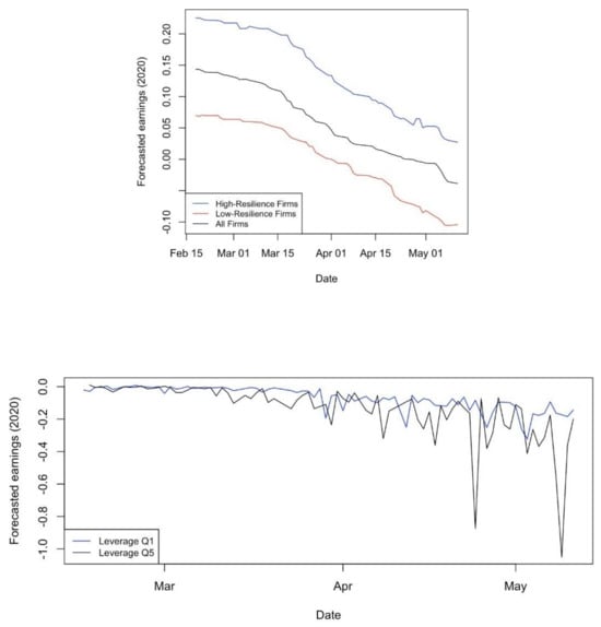
Figure 1.
The evolution of expected future cash flows in the fever period of COVID-19 (the impact of workplace resilience and leverage): The first panel shows the standardized earnings expectation of high- and low-resilience firms, in the sense of workplace flexibility, for current fiscal year of 2020. stands for an earnings expectation of firm i at time t (similar to Daadmehr, 2024; Koren & Pető, 2020; Landier & Thesmar, 2020). Firms with an ‘affected share’ less than 40 are assigned to the high-resilience group, and ones with greater than 65 are assigned to the low-resilience one. The second panel shows the standardized earnings expectations of firms with different levels of leverage. Firms with higher leverage than the 80th percentile are assumed high-levered (Q5), and firms with lower than the 20th percentile are the low-levered ones (Q1). Data source: Compustat/CRSP merged, WRDS for fundamentals, and Refinitiv-Eikon (Thomson Reuters) I/B/E/S forecasts for daily consensus analysts’ earnings.
Although this type of resilience is in accordance with the type of pandemic crisis and shows to what extent firms can survive when their productivity is affected by human loss (Koren & Pető, 2020), the financial status of firms can provide a type of flexibility for firms to handle additional production costs. In addition to all the evidence provided by Daadmehr (2024), the second panel of Figure 1 shows the analysts’ expectations of future cash flows separately for high- and low-levered firms and provides evidence of the importance of capital structure and firms’ leverage on the evolution of expected earnings. This panel exhibits that not only did earnings expectations decline more for high-levered firms, but also this decline for high-levered firms was persistent and associated with higher oscillations in the following fiscal years. This is consistent with much of the previous evidence that firms with less strong balance sheets experienced greater difficulties during and after the fever period of COVID-19, such as Pettenuzzo et al. (2023), which show how leverage and cash holdings are related to firm performance, especially those with less profitability and lower revenue growth. Each panel of this figure emphasizes that workplace resilience and firms’ corporate financials can separately explain heterogeneity in expected cash flows.
Meanwhile, firms with low workplace resilience would be more capable of handling and managing production costs if they already have a suitable financial position. They see less reduction in the average earnings expectations (Daadmehr, 2024); However, analysts were quite pessimistic about the rebound in earnings of these firms with lower financial status, as Daadmehr (2024) explains. So, it is crucial to find a mechanism in which these two intuitions jointly affect the expected cash flows and the price fluctuations of an equity claim to the output of such firms.
Figure 2 motivates and suggests the existence of such interaction. It shows the average earnings expectations for four categories of firms: “high workplace-resilience and high-levered” firms, “high workplace-resilience and low-levered” firms, “low workplace-resilience and high-levered” firms, and “low workplace-resilience and low-levered” firms. The evidence emphasizes two prominent impacts of firms’ financial status: (i) Among low-levered firms, those with a more flexible workforce not only have less reduction in average earnings expectations but also see less severe fluctuations in the following months after the onset (first panel). (ii) A higher leverage appears to weaken the benefit of high workplace resilience. The second panel, compared to the first one, suggests that high leverage reduces the earnings expectation surplus of high workplace resilience and makes fluctuations more severe. These two pieces of evidence highlight that firms’ financial characteristics can potentially magnify the impact of their workplace resilience on expected cash flows.
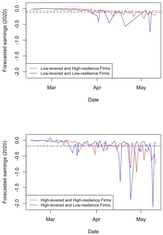
Figure 2.
The evolution of expected future cash flows in the fever period of COVID-19 (amplification effect): Both panels show the standardized earnings expectation, , for four groups of firms during the fever period. stands for the earnings expectation of firm i at time t for the current fiscal year of 2020. Firms with an ‘affected share’ less than 40 are assigned to the high-resilience group, and ones with greater than 65 are assigned to the low-resilience one. Firms with higher leverage than the 80th percentile are assumed to be high-levered, and firms with lower leverage than the 20th percentile are the low-levered ones. The categorization of firms into high- and low-resilience firms in the sense of workplace flexibility is based on Koren and Pető (2020) and follows Daadmehr (2024). Data source: Compustat/CRSP merged, WRDS for fundamentals, and Refinitiv-Eikon (Thomson Reuters) I/B/E/S forecasts for daily consensus analysts’ earnings.
3.3. Financial Resilience
Moreover, back to the story of the impact of a wide range of policies, any financial ratios from any category, including, e.g., profitability and solvency ratios, can be effective on all these associations. This re-motivates to quantify the overall impact of all corporate financials. This paper suggests a machine learning definition for financial resilience based on Dynamic Functional Principal Component Analysis (DFPCA) as a solution for such quantification (Section 4.2.2). The following sections show how cross-sectional time-varying dynamic functional PCs contribute to the asset-pricing model and to what extent financial resilience elements interact at the dividend level (Section 4.2) and possibly not only amplify the impact of workplace resilience, but also create significant heterogeneity in dividend growth (Section 6).
4. Model and Data
This section introduces the standard asset-pricing framework with the exogenous dividend stream, embedding the impact of COVID-19 on firms’ productivity. It clarifies how the paper quantifies resilience as well as how it controls the macro time effect of economic contraction. The data description is presented at the end of the corresponding subsections.
4.1. The Economy
The COVID-19 pandemic caused massive business disruption due to social distancing rules and lockdowns that almost all governments imposed. Specifically, firms in some industries were affected even more because they were not really flexible in their workforce, or they could not run tasks in the hybrid mode, simply because such tasks needed more human interaction or face-to-face communication with a higher physical presence. All of these increased the cost of production and affected the output of such low workplace-resilient firms. This situation created a sort of additional uncertainty in the market, which is quite important from an asset-pricing perspective. For a representative consumer (investor), it is important to know what happened to the price of an equity claim to the output of these firms.
Following Mehra and Prescott (1985) and Barro (2006), this paper considers recursive preferences of Epstein and Zin (1989) and Weil (1989) for representative-consumer Lucas’ fruit-tree model of asset pricing with an exogenous stochastic dividend stream4. Based on Campbell (1993) with total wealth at the beginning of t+1, as an intertemporal budget constraint and as the stochastic discount factor with time discount ; in partial equilibrium, the standard Euler equation is5:
4.2. Exogenous Dividend Stream
To clarify how resilience plays a role in the model, based on the initial evidence presented in Figure 2 and in line with evidence on the amplification effect (Daadmehr, 2024), this article defines the multiplicative form for the dividend level:
where captures the consequences of the COVID-19 disaster through not only the cross-sectional impact of this disaster on firms’ production, called workplace resilience, , but also the time-varying aggregate economic contraction, ; furthermore, refers to financial resilience, which is a linear combination of some functions of firm’s corporate financials. These terms are defined in the following subsections. The exogenous dividend growth for firm i at time t is:
In addition to , which is a normally distributed error term with mean zero and variance , in this article, the level of the impact of the exogenous COVID-19 disaster is multiplicative, although the growth rate is additive. This implies that the effect of this crisis on the stock price can be multiplicative, while that on returns may not be. In what follows, a full interpretation of the special feature of each element is presented.
4.2.1. Workplace Resilience: Cross-Sectional Effect of COVID-19
In the specification of dividend growth (Equation (3)), workplace resilience, , is introduced as the cross-sectional consequences of COVID-19, which refers to the characteristics of the firms in the workplace that determine the exposure of the firms’ dividend growth to this pandemic disaster. Koren and Pető (2020) show that this depends on a trade-off between the communication cost of firms and the benefits of the division of labor. They propose a measure for businesses, called “affected share”, including different aspects of workplace flexibility that represent customer-facing characteristics, degree of teamwork intensiveness, and workforce physical presence. Consequently, due to the nature of the COVID-19 pandemic that affects social interactions, this proxy reveals to what extent social distancing rules affect production costs.
captures the heterogeneous effect of workplace resilience of firm i, where is defined as workplace resilience and takes values of (100-“affected share”), a linear transformation of the proposed data of the “affected share” data by Koren and Pető (2020) for US companies in 3-digit NAICS sectors that practically captures heterogeneity caused by industry pandemic shock.
4.2.2. Financial Resilience: Dynamic Functional Principal Components
One of the main issues, specifically after COVID-19 emergence, is how to capture the compounding impact of different kinds of public policy, corporate policies, or even additional governmental packages, e.g., PPP in the case of the US. On one hand, such financial aids solve the problem of cash-flow shortage in the short term by liquidity injections, while on the other hand, these may change the capital structure. This is just a simple example to show the possible opposite outcomes mentioned in previous sections. Is it really possible to disentangle the single consequences of ALL these policies?
Having a huge database of cross-sectional, autocorrelated, and even lagged cross-correlated corporate financials incentivizes one to start organizing and reducing the dimension of massive data to obtain meaningful information on the financial status of firms. Corporate financials, like many other phenomena, can be considered as random curves, a kind of functional data that are realized over time. This time-varying intrinsic feature avoids using ordinary static data dimension-reduction methods such as Principal Component Analysis (PCA), which possibly ignores the essential information or correlation dependence in financial data. Moreover, Functional PCA (FPCA) still works in a static way and fails to capture serial dependence in random curves of corporate financials, and a lot of vital information about past values of functional observations is lost. The FPCA is still not able to capture the possible lagged cross-correlations among financial ratios.
This research employs Dynamic Functional PCA (DFPCA) provided by Hörmann et al. (2015), who respond to this demand with an efficient reduction technique. They propose a functional setup for a dynamic version of Karhunen–Loeve expansion and enhance the dynamic PCA originally suggested by Brillinger (2001). To obtain meaningful information on the financial status of firms as part associated with an amplification of dividend growth, this paper computes dynamic functional principal components as elements of “Financial Resilience”, representing the firm’s financial characteristics.
At the firm level, is defined as a matrix of d time series of the firm’s financial ratios. The m-th dynamic functional principal component is defined as:
where is the corresponding filter sequence (among all Brillinger, 2001). m varies from one to a maximum value of M, representing the number of principal components, which can explain the major variation originating from all financial ratios of firm i over time.
To obtain these dynamic functional principal components for each firm i, first, the empirical spectral density of is computed. The estimator is the estimated spectral density evaluated at the k-th frequency6:
where , , and the filter sequence, in Equation (4), are the Fourier coefficients of the dynamic eigenvector of the spectral density ; that is:
for , and . Then, the firm’s financial resilience, in Equation (3), is defined as a linear combination of the first M dynamic functional principal components, in Equation (4):
More statistical details are beyond the scope of this paper. The methodology for -curves can be directly found in Hörmann et al. (2015) and its appendices and online supplementary document. To compute the m-th dynamic functional principal component, Equation (4), this paper considers all monthly financial ratios of U.S. firms from 2013–2022, available at the WRDS database, belonging to all categories: capitalization, efficiency, profitability, liquidity, solvency, valuation, and financial soundness. Table A5 in the Appendix A provides detailed definitions.
4.2.3. Macro Time Effect of COVID-19
An overall time effect of exogenous COVID-19 is defined as , which controls common effects for the economic consequences of exogenous COVID-19 and the recession on all firms. This paper expands the methodology in Barro (2006) and considers economic contraction as a stochastic process rather than a single random variable, to obtain the estimates 7, based on monthly GDP data. Since the emergence of COVID-19 as a health crisis and its consequences on the demand and supply side impose regime shifts in the economy, the impact of economic contraction captured by GDP evolves with a nonlinear mechanism, in the sense that the response of GDP as a proxy for macroeconomic sensitivity to COVID-19 at time t depends on the state of the economy and its duration, which is not a simple linear function of the previous amount of GDP, but the change in coefficients by switching the state8. When the economy is subject to regime shifts, Markov-switching autoregressions (MS-AR) are the dominant research strategy in empirical macroeconomics.
Accordingly, the evolution of the monthly GDP, , is the Markov-switching process that switches among different unobservable states of the economy, . Let G denote the number of feasible regimes, so that , which indicates the regime prevailing at time t. By definition, the conditional probability density of is given by:
where is the autoregressive parameter in the regime and are realized at time t. Thus, for a given regime , is generated by an autoregressive process of order b, AR(b), such that the estimated fitted values, , are
Since the autoregressive process is defined based on unobservable states (Equation (6)), it is necessary to complete the data-generating mechanism with the regime-generating process, which is usually assumed to be a discrete-time and discrete-state Markov stochastic process defined by the transition probabilities.
To estimate the parameters of autoregression (Equation (7)) and the transition probabilities governing the Markov chain of the unobserved states based on observed information (monthly GDP), it is essential to calculate the desired conditional regime probabilities given a specified observation set (observed GDP), as the following.
To achieve this, the joint probability distribution of and states can be obtained as
The maximization of the likelihood function of MS-AR model can be carried out by an EM algorithm (among all Dempster et al., 2018; Hamilton, 1990; Krolzig, 1997) where at the “Expectation” step, an estimate of of an unobserved state variable , which records the history of Markov chain and , is updated using the estimated MS-AR parameters obtained at the last maximization step. In the “Maximization” step, the likelihood function, including these updated is maximized and gives the updated estimates for MS-AR parameters for the next expectation step. The EM algorithm continues, while the likelihood function increases at each step. For simplicity, these estimated state probabilities at time t given a specified observation set of (realized monthly GDP) are denoted by .
Section 6.1 and the robustness checks provided in Appendix A (Figure A1 and Table A1), specifically Table A2 and the computed Bayes factors (Chib, 1998), suggest a two-state MS-AR(1) to obtain the estimated state probabilities, , and the estimated economic contraction, 9. These re-notated probabilities, , allow us to simplify the notation of the estimates, , in Equation (7) for the next sections and asset-pricing model solution, as the following
indirectly depends on the state of the economy , through , fitted values of the MS-AR process. Section 6 proposes the most appropriate regime-switching specification and estimates a two-regime MS-AR(1).
This paper uses normalized seasonally adjusted monthly GDP in the US10 from 1960 to 2022 to estimate the probability of states and to compute the fitted values , as an estimation of overall economic contraction due to COVID-19. The impact of COVID-19 is completely different from not just the impact of the financial crisis of 2008 and the 2011 European crisis, but also the impact of previous wars. Based on Jordà et al. (2022), wars and disease crises, as two main types of crises, have different economic consequences. This motivated us to concentrate on only the COVID-19 period. On the other hand, there are 9 years of data free from the impact of any other crisis (2013–2022). This is a splendid opportunity to investigate the impact of COVID-19 as an exogenous health shock. In Section 6.2, this paper considers from 2013 to 2022 in order to estimate the proposed dividend stream.
4.2.4. Dividend Growth
To sum up this section and obtain the price of an equity claim, the dividend growth is proposed by replacing Equation (5) in Equation (3)11, as follows:
In order to estimate dividend growth and establish the resilience heterogeneity as well as obtain calibrated parameters in the model-based equity premium (the solution of the model is provided in the following section), this paper estimates and as fixed coefficient effects and as a random coefficient effect in a mixed-coefficient generalized linear model framework12. To mention the importance of that captures the overall impact of workplace resilience across firms, it is worth highlighting that this term is actually an interaction between the statistical model13 and workplace resilience as a variable with a heterogeneous impact on dividend growth. The empirical results, in Section 6, clarify the key role of this random coefficient effect as the heterogeneous impact of workplace resilience by estimating using the Restricted Maximum Likelihood method, REML. For a theoretical interpretation of mixed-effect specifications, this paper refers directly to (Baayen et al., 2008; Gelman, 2005; Henderson, 1982), since more statistical details are beyond the scope of this paper.
This study uses Computstat/CRSP merged for monthly fundamentals and financial ratios available at WRDS, for US firms from 2013 to 2022.
In the next section, the solution of the model and asset-pricing implications for the COVID-19 disaster are presented based on the estimation of Equation (8) as the dividend stream.
5. Solution of the Model
Given the exogenous dividend stream in Equation (8), and the assumed distribution for the error term (Section 4.2.4), the price-to-dividend ratio is14:
The expected return can be defined as and computed as:
Moreover, the return on risk-free assets is:
Then, the equity premium is given by:
This paper considers that the time discount factor is 0.999, consistent with many articles (among all Wachter, 2013). The probability of a disaster state, , is estimated monthly based on the methodology provided in Section 4.2.3 and the parameters, , , are estimated using a random coefficient generalized linear model (Section 4.2.4). After estimating MS-AR(1) in Section 6.1 and the exogenous dividend growth over 2013–2022 in Section 6.2, the article performs a calibration exercise for , and using the price-to-dividend ratio, the risk-free rate, and the following model-based Sharpe ratio.
where is the discount factor presented in Section 4.1, and
This setup obtained and elasticity of intertemporal substitution (EIS), . This calibration exercise for relative risk aversion and EIS implies that generally speaking, investors became a bit more conservative in the COVID-19 situation, in the sense that the representative investor might prefer the early resolution of uncertainty, since (Bansal et al., 2012)15. Moreover, the calibration suggests a reasonable value of 7.3 for , in line with the fact that not only uncertainty but also even a very small possibility of disaster makes the dividend growth have a heavier tail distribution. This highlights the impact of a “rare” disaster in line with Weitzman (2005) and reveals the impact of COVID-19 as a rare event on the distribution of dividend growth.
Based on all estimated and calibrated parameters, Figure 3 plots the model-based asset-pricing implications (the tractable formulas) as a function of the disaster probability spanned in [0, 1]. It shows the price-to-dividend ratio and the risk-free rate as increasing and decreasing functions of disaster probability, respectively. In periods with a higher probability of disaster, a decline in dividends occurs at a faster pace than a price reduction, since it is assumed that the price is a discounted future dividend stream, including some “no-disaster” states. The first panel illustrates that when the possibility of disaster is higher than 0.85, dividends plunge to zero, and the price-to-dividend ratio becomes strictly increasing at the highest pace.
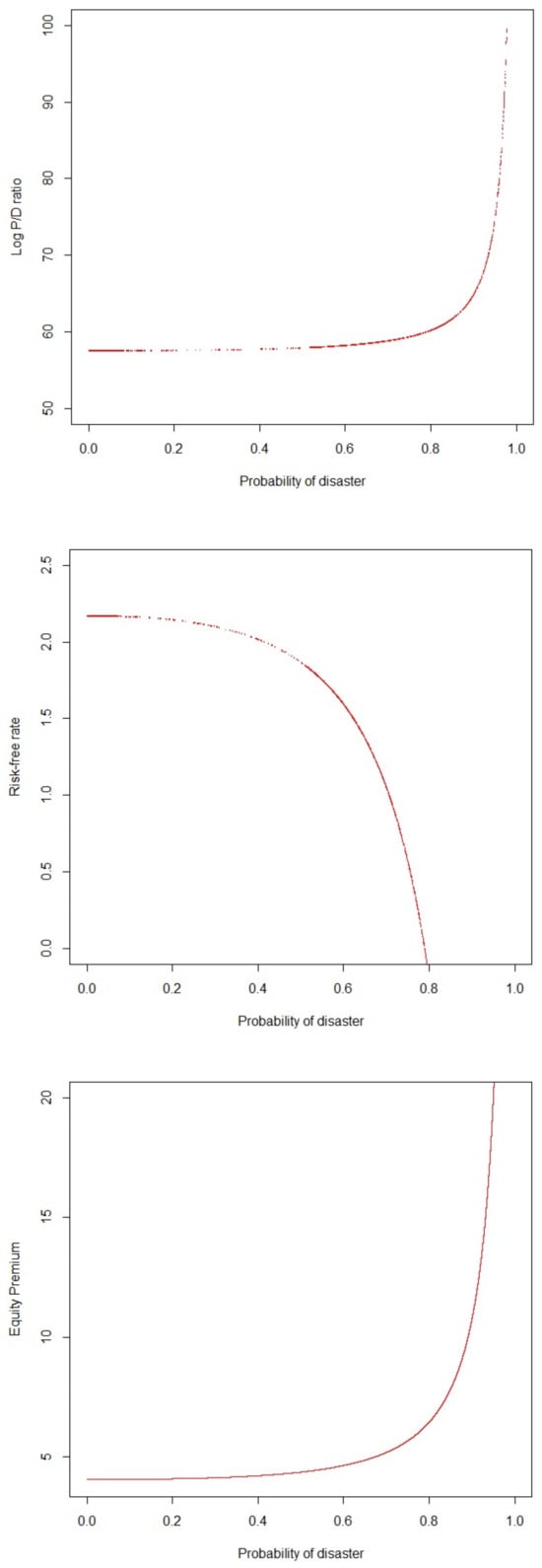
Figure 3.
Price-to-dividend ratio, risk-free rate, and equity premium: This figure plots the log P/D ratio, log risk-free rate , and equity premium as a function of probability of disaster. The log P/D ratio, log risk-free rate, and equity premium are computed based on estimated parameters , , (Section 6) and calibration exercise for , , and . Data source: Compustat/CRSP merged and financial ratios, WRDS.
In case of the possibility of disaster, there is an interest in buying more risk-free assets, their price goes up, and the risk-free rate decreases. The second panel shows that the model-based risk-free rate is decreasing in the probability of disaster. Clearly, in case of a very high probability of a disaster state, there is no interest in the risky asset, so the equity premium increases as compensation to cover the additional risk. The third panel shows that the model-based equity premium is an increasing function of the probability of disaster. Moreover, in line with Barro (2006), the equity premium is a decreasing function of risk aversion . In what follows, the paper presents the estimation of exogenous dividend growth and its parameters used in the calibration exercise.
6. Results
This section presents an estimated exogenous dividend stream for model-based asset-pricing implications. The first part (Section 6.1) clarifies that COVID-19 is a disaster and provides the estimation of the macro time effect of COVID-19 () from 2013 to 2022, the period over which the exogenous dividend stream is estimated. The second step (Section 6.2) quantifies the impact of financial resilience components. It also estimates dividend growth (Equation (8)) as well as the fixed-effects and s, which are coefficients of macroeconomic contraction, , and financial resilience components, , respectively, and as the heterogeneous effect of workplace resilience, , using the Restricted Maximum Likelihood method, REML, over 2013–2022.
6.1. Macroeconomic Sensitivity to COVID-19 Disaster
In the proposed approach, the first step is to estimate the macroeconomic contraction due to COVID-19 to control for the aggregate time effect, as explained in Section 4.2.3. Figure 4 shows the fitted two-regime Markov-switching (MS) model for the monthly GDP of the United States from 1960 to 2022 and specifies the disaster regimes. This figure provides an opportunity to empirically prove that this pandemic was a disaster with significant macroeconomic consequences and exhibits the COVID-19 pandemic period as a disaster regime. Furthermore, according to Table 1, the estimation for controlling the macro time effect of COVID-19, , can be obtained from:
with the estimated transition probabilities in Table 2. The significant switching AR(1) coefficients in Table are a sign of severe economic contraction in disaster states, specifically, the estimated coefficient in disaster states (1.03) shows that such a macro time effect is not mean-reverting in disasters.
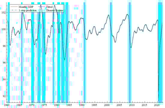
Figure 4.
Monthly GDP, fitted the two-regime MS-AR(1) and the one-step prediction from 1960 to 2022: The blue columns show the disaster regimes (states and the duration). Data source: normalized seasonally adjusted GDP, Federal Reserve Bank of St. Louis, Economic Research Division.

Table 1.
Estimated parameters of MS-AR(1): This table presents the maximum likelihood estimation of the two-regime Markov-switching AR(1) and the conditional probability of disaster states. It provides the Likelihood Ratio Test to examine linear vs. nonlinear two-regime MS-AR(1). Significant codes: 0 ‘***’, 0.001 ‘**’.
Table 2.
Estimated transition matrix: This table shows the conditional probability of disaster states estimated by two-regime MS-AR(1).
The LRT statistic provided in Table empirically proves the significance of nonlinear two-regime MS-AR(1). The evidence on optimal choice of the number of regimes is presented in Table A1 and Table A2 in Appendix A.
Figure 5 shows the evolution of the probability of a disaster state, . As can be clearly seen and in line with Figure 1, the probability of a disaster state increased to around 0.9 in the fever period of COVID-19, followed by a reduction due to the impact of good news about vaccines. Although the probability of a disaster state at time t being conditional on the non-disaster state for the previous month is 2 percent, which is in line with the calibrated static disaster probability of 1.7 percent proposed by Barro (2006), the economy will remain in the disaster regime due to the low transition probability of 8 percent. Table 2 shows that switching from disaster states to non-disaster ones happens with a probability of 0.08.
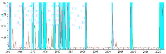
Figure 5.
Evolution of estimated probability of disaster state based on MS-AR(1), from 1960 to 2022:The blue columns show the disaster regimes (states and the duration).
In addition to Figure 4, which graphically shows the goodness of fit and the appropriateness of the estimated economic contraction, , Table A3 (in the Appendix A) verifies these results and contains not only the estimated disaster states and the duration of the regimes, but also the evidence from the Fed reports. It compares the estimated disaster regimes with the corresponding actual events. The estimation of disaster regimes accords with the historical information in (Burger, 1969; Hoxworth et al., 1983; Supel, 1978).
Moreover, Figure A1 (in the Appendix A) shows the estimated distribution for macroeconomic sensitivity, , and compares the bimodal distribution with the corresponding normal distribution. It provides another form of verification of the number of regime switches.
6.2. Justification for Dividend Stream and Asset-Pricing Moments
To interpret the impact of corporate financials and to investigate whether and to what extent the financial status of firms amplifies the consequences of COVID-19 on asset prices, this paper starts with around 70 financial ratios of 5833 US firms over 2013–2022 at monthly frequency and employs Dynamic Functional Principal Component Analysis (DFPCA) to capture the impact of firm’s financial status, as explained in Section 4.2.2.
By computing the filter sequences and dynamic functional principal components, it is possible to provide the scree plot and decide on the number of components required to include most of the variation originating from all corporate financials that possibly affected dividend growth. Figure 6 shows the portion of variance explained by each dynamic functional PC for all firms, separately, in one diagram. It suggests that the first five components explain the most variation (over 90 percent) induced by financial ratios for almost all firms.
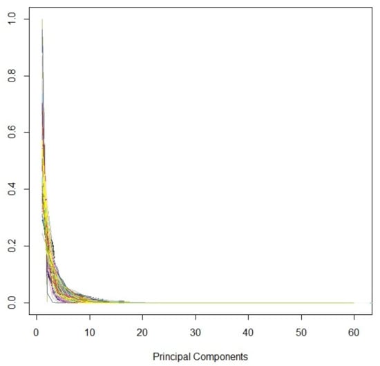
Figure 6.
A scree plot of the Dynamic Functional Principal Component Analysis (DFPCA) of financial ratios: This figure shows the portion of variance explained by each component (eigenvalues). Each colored line is the scree plot of one firm, separate from others. The sample contains around 5833 US firms. Data source: firm-level financial ratios, WRDS.
Based on Equation (8) and the first five dynamic principal components (PCs)16, the results of the estimated dividend growth are summarized in Table 3. This table presents the quantified effect of workplace resilience and the impact of the firm’s financial resilience as the elasticity of dividend growth to these two intuitions of resilience.
Table 3.
Dividend growth estimation: This table provides estimation for coefficients of financial resilience components and the impact of COVID-19, including the macro time effect of COVID and workplace resilience (Equation (8)). It presents the fixed-effects of the first five cross-sectional time-varying dynamic functional PCs and the heterogeneous effect of workplace resilience , by REML estimating method. The industry sector codes from “2” to “6” belong to “Mining, Utility and Construction”, “Manufacturing”, “Trade, Transportation and Warehousing”, “Information, Finance, Management, and Remediation Services”, “Educational, Health Care and Social Assistance”, respectively. Each column shows the estimated result for each industry separately. The numbers in parentheses are standard deviations of corresponding estimated coefficients. Significant codes: 0 ‘***’ 0.001 ‘**’ 0.01 ‘*’ 0.05.
6.2.1. Interpretation of Workplace Resilience Impact
It can be clearly seen that the workplace resilience has a significant positive average heterogeneous effect of 10.36 on dividend growth for a sample of all industries. For individual industries, the corresponding coefficient of workplace resilience in the specification of dividend growth varies on average from 2 to 14, respectively, in “Mining, Utility and Construction” and “Information, Finance, Management, and Remediation Services”. The key result on the average heterogeneous effect of workplace resilience can be seen in Figure 7. Based on workplace resilience, firms are categorized into two, three, and four groups. In each case, the first and last groups are considered low- and high-resilience firms, respectively. This figure indicates that the average heterogeneous effect of workplace resilience for low-resilience firms is greater than the one for high-resilience firms (the red line is below the blue line in Figure 7), meaning that the elasticity of dividend growth with respect to workplace resilience for firms with a very low degree of workplace resilience is much higher than the one for very high-resilience firms. On the other hand, it can be clearly seen in Figure 7 that the greater the difference in the workplace resilience of firms (an increase in the number of groups, equivalently), the greater the difference in the averaged heterogeneous effect or the corresponding elasticity (an increase in vertical distance between the red point and the blue one); as a result, for the same amount of increase in workplace resilience, there is a greater change in dividend growth of low-resilience firms based on Equation (8). Daadmehr (2025) theoretically proves a similar statement for expected returns and shows that an increase in COVID intensity increases the expected return of low-resilience firms much more than that of high-resilience firms.
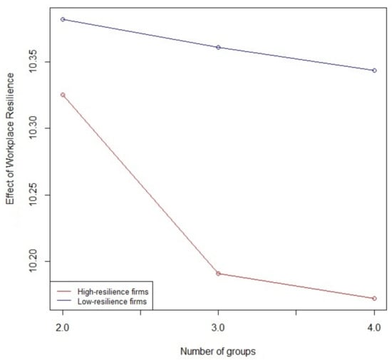
Figure 7.
The average heterogeneous effect of workplace resilience: This figure exhibits how the difference in workplace resilience of high- and low-resilience firms changes the average heterogeneous effect of workplace resilience, by sorting and equally splitting firms into K groups based on their workplace resilience. The first group and the last one are considered firms with low and high workplace resilience, respectively.
To sum up, Figure 7 suggests that in low-resilience firms, a one-percent improvement in workforce flexibility increases dividend growth much more than in the case of high-resilience firms, since the average estimated heterogeneous coefficient for low-resilience firms is much higher. Summary statistics and empirical results on the heterogeneous effect of workplace resilience are provided in Table 4. This table provides statistical tests to reveal these differences in heterogeneous effect, , for these two groups of firms. The results in this table implicitly examine the significant differences in the elasticity of dividend growth to workplace resilience between high- and low-workplace-flexible firms. This table empirically proves that for any number of groups (K), the heterogeneous effect of the workplace resilience of high workplace-resilient firms is “significantly” different from that of the low workplace-resilient ones. Consequently, there are significant discrepancies in dividend growth of high- and low-resilience firms created by the heterogeneous effect of workplace resilience. In other words, this indicates that dividend growth for low-resilience firms is significantly more sensitive to workplace resilience than that of high-resilience firms, technically proving the existence of significant resilience heterogeneity in expected cash flows.
Table 4.
The summary statistics of heterogeneous effect of workplace resilience: This table provides the summary statistics on the heterogeneous effect of workplace resilience for high-resilience and low-resilience firms, including the results of group comparisons. Based on workplace resilience, firms are sorted and split into K groups. The first group and the last one are considered firms with low and high workplace resilience, respectively. It compares the heterogeneous effect of two groups of firms using the nonparametric Wilcoxon test. The heterogeneous effect of high-resilience firms is significantly different from the low-resilience ones (at the level of 0.001, indicated by ***).
6.2.2. Interpretation of Macro Time Effect of COVID-19
Table 3 emphasizes the importance of macroeconomic COVID sensitivity, which implies a significant reduction in dividend growth not only at the level of “All industries”, but also within each industry, except “Mining, utilities and construction”. The estimated coefficient of is statistically significant, showing that all sectors are significantly sensitive to the recession caused by COVID-19, except “Mining, Utility and Construction”.
Does the low amount of estimated workplace resilience, , imply such an insignificant effect of macroeconomic contraction due to COVID-19? In this sector, the reason for the lack of statistical significance of is related to the low amount of estimated average heterogeneous effect of workplace resilience of 2.6. Firms in this sector have a much lower average heterogeneous effect of workplace resilience compared to its average amount plotted in Figure 7 (the red line is below the blue line in Figure 7 and the average amount of 2.6 for this industry is much smaller than the average in the case of “all industries”, in Figure 7). Consequently, this suggests that firms in this industry are more workplace-resilient, on average. Hence, in this industry, social distancing restrictions are not as intrusive as they are in other sectors, so it is not surprising to see such an insignificant impact of the macro time effect of COVID-19.
6.2.3. Interpretation of Financial Resilience
Table 3 also shows the results of elements of financial resilience. The significance of dynamic functional principal components of financial ratios not only suggests the significant effect of firms’ financial status on dividend growth but also proves the significant amplification of workplace resilience by corporate financials17, , in Section 4. This table reveals that financial resilience, especially the first two principal components, which contain most variations originating from financial ratios, directly affects dividend growth and makes its resilience more heterogeneous. These small estimated effects, , is not catastrophic in such a pandemic crisis but is significant enough. Then, overall resilience heterogeneity is not just from the workforce resilience perspective but also based on what firms financially experienced before and during the COVID-19 outbreak. The next section introduces the major elements with more contribution to firms’ financial resilience.
On top of all this, since the averaged heterogeneous effect of workplace resilience is greater than the estimated coefficients of financial resilience elements (PCs), dividend growth is more elastic and responsive to workplace resilience. Equivalently, the role of workplace flexibility is more prominent in explaining the resilience heterogeneity in dividend growth.
Moreover, the empirical results in this section show “to what extent” cash flows can be resilience-heterogeneous and the solution of the proposed model in Section 5, sheds light on “how” such significant resilience-heterogeneity, specifically the heterogeneous effect of workplace resilience and the amplification effect by financial resilience, can be transferred to expected returns as well as all asset-pricing implications. The calibrated exercise compares model-based asset-pricing moments with the corresponding values from historical data. The model-based equity premium (5.269) is close to the average equity premium from the data (5.147). The result holds for the risk-free rate (1.137 vs. 1.006 from historical data). The model-based standard deviation of the log risk-free rate (2.531) is in line with the corresponding amount presented by Ghaderi et al. (2022) using historical data from 1950 to 201918.
7. Major Elements of Financial Resilience
Section 6 explained the significant role of financial resilience of assets in amplification of the dominant heterogeneous effect of workplace resilience on exogenous dividend growth, as well as asset-pricing implications (Section 5). The key application of Dynamic Functional Principal Component Analysis (DFPCA) determined the first five major PCs as components of financial resilience , at the firm level over time, including the COVID-19 era. This section clarifies which financial ratios mostly drive fluctuations in these firms’ financial resilience components.
Figure 8 shows the weights of the financial ratios for each of . It provides an opportunity to compare the relative importance of financial ratios in determining the firm’s resilience. This figure reveals major ratios with over 90 percent average weight (above the black dash line) in the specification of at least one of the first five principal components, , for . It determines Shiller’s Cyclically Adjusted P/E Ratio, Price/Operating Earnings (Basic), Price/Operating Earnings (Diluted), P/E (Diluted, Excl. EI), P/E (Diluted, Incl. EI) and Price/Sales (valuation ratios); Cash Conversion Cycle (liquidity ratio); and Interest Coverage Ratio (solvency ratio) as main elements of dynamic functional PCs and financial resilience as well.
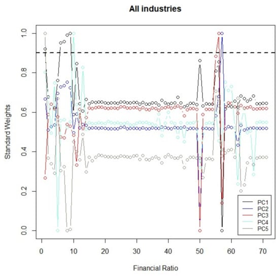
Figure 8.
Overall weights of financial ratios (average of filter sequences, , for the first five PCs): This figure shows the standardized weights of all financial ratios obtained by DFPCA. The sample contains 5833 firms in all industries. The black dash line is the threshold of 90 percent for weights. Data source: firm-level financial ratios, WRDS.
Daadmehr (2024) explains to what extent the valuation and liquidity ratios are significantly correlated with the proposed financial-based resilience index and emphasizes the necessity of workplace flexibility to define a novel “Composite-Financial Resilience Index”. The machine-based (DFPCA) choice of valuation ratios is in line with Glossner et al. (2024), who emphasize the important amplification role of institutional investors in valuation and the severe price decline in COVID-19. Furthermore, having a liquidity ratio as one of the important ratios determined by DFPCA is consistent with Pagano and Zechner (2022), who mention the significant change in liquidity levels of listed US firms from before the emergence of the pandemic to after the onset.
The choice of Interest Coverage Ratio is in line with Palomino et al. (2019), who interpret countercyclicality and its negative relationship with economic activity. In what follows, there is an interpretation of the relation between these ratios, workplace resilience, and firms’ vulnerability and riskiness.
7.1. Valuation Ratios
By definition, valuation ratios are appropriate to measure the relationship between market value and some stream of fundamentals. Figure 9 shows the time variation in different types of valuation ratios with higher than 90 percent weight (averaged in Equation (4)) in elements of firms’ financial resilience () after the onset of the COVID pandemic, diagnosed by Dynamic Functional PCA (DFPCA). The first panel shows that the time trend for almost all of these ratios is the same, especially different types of price-to-earnings ratios that are commonly used as good financial metrics to obtain a better understanding of the overall picture, and are accessible to a wide range of investors. In this paper, DFPCA technically proved its significant role in resilience-heterogeneous dividend growth through the firm’s financial resilience (Section 6.2).
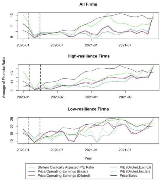
Figure 9.
Valuation ratios: This figure shows the time series of major valuation ratios determined by Dynamic Functional Principal Component Analysis. The categorization of firms into high- and low-resilience groups, in the sense of workplace flexibility, follows Koren and Pető (2020) and Daadmehr (2024). Firms with an ‘affected share’ of less than 40 are assigned to the high-resilience group, and ones with greater than 65 are assigned to the low-resilience group. Vertical black dash lines refer to the fever period of the COVID-19 pandemic, from February to April 2020. Data source: firm-level financial ratios, WRDS.
This figure compares the descriptive behavior of these valuation ratios, also separately for high- and low-resilience firms (the second and third panels), in the sense of workplace resilience. It can be clearly seen from the second panel that these ratios have a more homogeneous trend for high-resilience firms. This homogeneity is less clear in the case of low-resilience firms. To make a better comparison between the valuation ratios of high- and low-resilience firms, one of these ratios is selected as a representative. The Dynamic Functional PCA determines “Shillers Cyclically Adjusted P/E Ratio” as an effective main element of either or with a weight of more than 90 percent (Figure 8). In particular, DFPCA implicitly mentions the inflated P/E due to low or even negative earnings during economic downturns like COVID-19 and refers to the cyclicality of earnings during these periods. It highlights the importance of cyclically adjusting P/E and selects “Shillers Cyclically Adjusted P/E Ratio” as the most promising valuation ratio among different definitions of P/E ratio. The first panel of Figure 10 shows that the adjusted P/E ratio for low-resilience firms is higher than that of high-resilience firms during the COVID-19 outbreak, except for a short time at almost the end of the fever period in the first wave of this pandemic. The flip point in the fever period is consistent with Pagano et al. (2023).
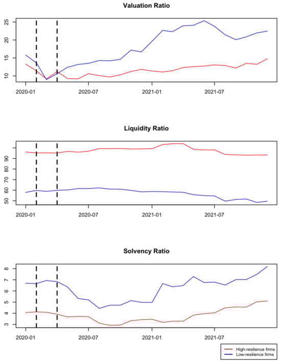
Figure 10.
Representative financial ratios: This figure shows the time series of Shiller’s Cyclically Adjusted P/E (valuation ratio), Cash Conversion Cycle (liquidity ratio), and Interest Coverage Ratio (solvency ratio) as major elements determined by DFPCA. The categorization of firms into high- and low-resilience groups, in the sense of workplace flexibility, follows Koren and Pető (2020) and Daadmehr (2024). Firms with ‘affected share’ less than 40 are assigned to the high-resilience group, and ones with greater than 65 are assigned to the low-resilience group. Vertical black dash lines refer to the fever period of the COVID-19 pandemic, from February to April 2020. Data source: firm-level financial ratios, WRDS.
Generally speaking, when a firm has a high P/E ratio, it implies that investors are willing to pay a premium for its stock relative to its current earnings. Although high P/E ratios signal growth expectations, they also introduce risk. Investors should carefully take these risks into account in their investment decisions. Simply, a firm with a high P/E ratio can be seen as risky for several reasons: (i) Uncertainty: The stock price may suffer if the company fails to meet those expectations. (ii) Market Sentiment: Any negative news can lead to a sharp decline in the price of stock with higher expectations. Then, investor sentiment plays an important role. (iii) Volatility: The price of stocks with high P/E ratios reacts more strongly to market events. (iv) Missed Expectations: It is disappointing for investors if the company loses its growth targets, leading to a potential sell-off.
Firms with higher P/E ratios can possibly be considered riskier since they have higher growth expectations19, making them more vulnerable, as explained. So, stocks with lower P/E ratios may be perceived as less risky, but this is not sufficient enough to assess the overall firm’s financial status and health. Figure 10 (first panel) explains that these firms with higher adjusted P/E ratios are low-resilience in their workforce, in line with Daadmehr (2024), who empirically proves that low-resilience firms are riskier and naturally investors expect more returns on these stocks.
Firms can control the level of the P/E ratio through different kinds of policy. Many articles investigate the impact of dividend policy on the price-to-earnings ratio. Among all, Jitmaneeroj (2017) discusses how these policies and the P/E ratio have a negative and positive association depending on the firm’s profitability. Despite the sticky preferences for dividend policy, many papers explain the existence of determinants that affect firms’ decisions on this kind of policy. One growing strand of the literature suggests that dividend policy can be influenced by ownership structure and affect firms’ performance. Lopes and Narciso (2020) examine the ability of earnings management practices to predict the dividend policy and suggest ownership concentration as a main driver of this relationship. Furthermore, the association between insider ownership and financial performance affects the firm’s P/E ratio. Houmes and Chira (2015) explain that high insider ownership makes the board ineffective and perpetuates weak performance with lower P/E, showing that managers are not capable enough to create value and firms are riskier in this sense, and investors require higher returns.
On another front, accounting and investment policies can jointly affect the P/E ratio. Staehle and Lampenius (2013) compare firms with different accounting and investment policies and combine a model with overlapping capacity investments (among all, Rogerson (2008)).
However, this ratio itself cannot be representative of corporate financials, such as the level of the firm’s debt or cash flow. This emphasizes the necessity of quantifying financial resilience , as an overall indicator of corporate financials, and refers to its important role not only in exogenous dividend growth but also in asset-pricing implications. This directly highlights the novel application of Dynamic Functional PCA as a new definition of financial resilience.
7.2. Liquidity Ratio
Another important element with over 90 percent weight in dynamic functional PCs ( according to Figure 8) is the “Cash Conversion Cycle (CCC)” which can be an indicator of liquidity risk, operational efficiency, and overall financial status. This indicator represents the number of days needed to convert resources to cash. The fewer days it takes, the better it is for the business. The second panel of Figure 10 indicates that, not surprisingly, there is almost no fluctuation in this kind of liquidity ratio in the case of high- or low-resilience firms in the sense of workplace flexibility. However, this panel reveals a huge cross-sectional difference between these two groups of firms in the number of days it takes to convert the cash spending on inventory back into cash by selling its product. This refers to the novel application of Dynamic Functional PCA that can simultaneously capture not only time variation but also cross-sectional heterogeneity in corporate financials.
Holding physical inventories is not a big issue for highly workplace-resilient firms who are capable enough to run distance-working plans and consequently, no matter to what extent conversion takes time. As expected, for high-resilient firms in the workplace, the conversion period is longer since the cash cycle is not a significant consideration for such firms (second panel of Figure 10). On the other hand, firms with low workplace resilience are riskier in the presence of COVID-related lockdown periods (Daadmehr, 2024) and they face more workplace disruption, since it is not possible to conduct different tasks in hybrid mode. Therefore, firms with low workplace resilience need more liquidity and so put more effort into cash-cycle reduction by improving performance in Days Payable Outstanding (DPO), Days Sales Outstanding (DSO), and Days Inventory Outstanding (DIO)20.
Since the Cash Conversion Cycle depends on industry type, management, and many other factors, it is not an appropriate representative measure of firms’ performance and should be considered with other performance criteria. This is exactly what this paper pays attention to. The financial resilience () part of exogenous dividend growth provides a hybrid quantification of firms’ financial status.
7.3. Solvency Ratio
These types of financial ratios help to determine the short-term financial health of a firm, and investors and lenders use them to determine the risk of lending money to the firm21. Another major element with over 90 percent impact on the financial resilience components of firms is the “Interest Coverage Ratio (ICR)” that plays an important role in the cross-sectional and time variation in the third dynamic functional (Figure 8). This evidence is in line with studies that show there is a large cross-industry variation in ICR in different industries, which signals a deterioration of corporate financial conditions (Palomino et al., 2019).
The third panel of Figure 10 reveals a decrease in the level of ICR starting from April 2020. A declining ICR indicates that firms may not be capable enough to meet their debt obligations in the future and become more risky. In COVID time, low-resilience firms were riskier since their workplaces were not flexible enough under the new social distancing rules. These industries saw business disruptions and became even more financially vulnerable in the COVID era (Daadmehr, 2024; Koren & Pető, 2020; Pagano et al., 2023). After April 2020, the decline in ICR for low-resilience firms was greater than that of the high-resilience firms, showing that low-resilience firms had more difficulties meeting their debt obligations.
As explained, low-resilience companies in the workplace are more risky (Daadmehr, 2024) due to the impact of the exogenous COVID-19 pandemic. Risky industries with limited access to external debt financing (e.g., Computer Equipment or Chemicals) require even higher ICRs to be considered creditworthy and financially stable. The third panel of Figure 10 exhibits the persistent higher ICR for firms with low resilience in the workplace that are more risky during all periods of the COVID-19 outbreak (Daadmehr, 2024) and suggests that this workplace riskiness can be amplified by the impact of ICR. The results in Section 6 empirically prove such significant amplifications in exogenous dividend growth. The novel asset-pricing model and the solution in Section 5 reveal how such significant amplification affects expected returns.
The vital role of all three types of financial ratios strictly emphasizes the need for a setup that shows how the financial status of firms interacts with workplace resilience and plays an asset-pricing role in the time of COVID-19. The novel application of Dynamic Functional Principal Component Analysis highlights the major and significant role of these valuation, liquidity, and solvency ratios (among all others) in the snapshot of firms’ financial status, as well as asset-pricing implications (Section 5 and Section 6.2).
8. Conclusions
In this paper, the key aspect of the empirical results is twofold. First, results on the heterogeneous effect of workplace resilience assert that not only does this type of resilience have a direct positive relation with dividend growth, but also the dividend growth for high-resilience firms has less sensitivity to workplace resilience as opposed to low-resilience firms. More importantly, the low amount of averaged heterogeneous effect in some industries can be a sign of a high degree of workplace resilience, as well as insensitivity to aggregate time-varying economic contraction of the COVID-19 disaster.
This study answers the ambiguity of the amplification effect of financial resilience on asset prices mentioned by Daadmehr (2024), by quantifying this kind of resilience and taking the firm’s financial status into account in an appropriate mechanism for asset-pricing models. The methodology in this part clearly reveals how the amplification effect of corporate financials has a significant impact on the dividend stream. To understand to what extent such amplification affects the asset-pricing implications, the paper estimates dividend growth and calibrates preference parameters based on a novel extension of Barro (2006), including the workplace resilience (Koren & Pető, 2020) and financial resilience components. The estimated dividend growth highlights that although the impact of firms’ financial resilience is statistically significant, the effect of workplace resilience is dominant.
The novel application of Dynamic Functional Principal Component Analysis deconstructs the impact of financial resilience and reveals the major and significant role of valuation, liquidity, and solvency ratios in not only the amplification of the COVID effect, especially the impact of workplace resilience, but also exogenous dividend growth and equity premium in a tractable formula. The results emphasize the necessity of financial resilience components (dynamic functional PCs) as a novel definition that could capture time-varying and cross-sectional variation in all corporate financials.
Second, this paper presents an opportunity to assert and prove that COVID-19 is not only a health crisis, but can also be considered a disaster with significant macroeconomic consequences. The results of the Markov-switching approach establish the significant economic contraction during COVID-19. The most prominent result on this part is related to estimating the probability of disaster that has a direct impact on the model-based equity premium (Equation (9)). The estimated macroeconomic sensitivity to the COVID-19 disaster shows a negative impact on dividend growth. By controlling the overall economic contraction due to COVID-19, this paper presents the asset-pricing implications of the COVID-19 disaster. The tractable formulas reveal how equity premium can be characterized by different cross-sectional and time-varying sources of variation; specifically, the model shows that the equity premium is an increasing function of disaster probability. The exercise in calibration, especially the standard deviation of dividend growth, explained the impact of COVID-19 as a disaster on dividend growth distribution that agrees with Weitzman (2005), who emphasizes the impact of rare events to have a heavier tail distribution.
The asset-pricing model developed in this paper can be applicable in any pandemic-like disaster when workplace sustainability drives investors’ beliefs and plays a key role in pricing mechanisms. This evidence sheds light on future research ideas to propose an asset-pricing model with rare events, including not only the COVID-19 disaster but also previous crises from WW1 to the Russia–Ukraine war. This agenda necessitates a longer discussion on how different kinds of disasters with different economic consequences can be considered under the broader setup of the asset-pricing model. This paper leaves this for future work.
Funding
Special gratitude is extended to the University of Naples Federico II for providing data, to the University of Padua, Department of Economics and Management “Marco Fanno” for research grants; and to the Vienna University of Economics and Business (WU-VGSF) for the visiting opportunity and for providing I/B/E/S forecast data from the Refinitiv-Eikon (Thomson Reuters) and WRDS databases.
Institutional Review Board Statement
Not applicable.
Informed Consent Statement
Not applicable.
Data Availability Statement
Datasets are partially available upon request.
Acknowledgments
Warm thanks to Marco Pagano, Josef Zechner, Antonio Acconcia, Daniele Massacci, Lorenzo Pandolfi, and participants at FMA European Conference 2024 (Doctoral Consortium), the International Risk Management Conference (IRMC2023), the Research Symposium on Finance and Economics (Krea University, RSFE2023), Riunione Scientifica Annuale, Societa Italiana di Economia (SIE-RSA2023), the 45th Eurasia Business and Economics Society Conference (EBES2023), seminars at the University of Padua (dSEA), the University of Naples Federico II (DiSES), and the Centre for Studies in Economics and Finance (CSEF).
Conflicts of Interest
The author declares no conflicts of interest.
Appendix A

Figure A1.
Estimated distribution of macroeconomic contraction : This figure compares the empirical distribution of the macro time effect of COVID−19 with the corresponding normal distribution.
Figure A1.
Estimated distribution of macroeconomic contraction : This figure compares the empirical distribution of the macro time effect of COVID−19 with the corresponding normal distribution.

Table A1.
Tests of Markov-switching non-linearity: This table compares the linear model with the Markov-switching model with different numbers of regimes, using the Likelihood Ratio Test. In all cases, the null hypothesis (linear model) is rejected at the level of 0.001.
Table A1.
Tests of Markov-switching non-linearity: This table compares the linear model with the Markov-switching model with different numbers of regimes, using the Likelihood Ratio Test. In all cases, the null hypothesis (linear model) is rejected at the level of 0.001.
| Model Comparison | Lin vs. MS(2) | Lin vs. MS(3) | Lin vs. MS(4) | Lin vs. MS(5) | Lin vs. MS(6) |
|---|---|---|---|---|---|
| LR-Test | 1102.7 | 1413.4 | 1710.0 | 1790.3 | 1813.5 |
Table A2.
Test for number of regimes in Markov switching: This table compares the non-linear Markov-switching model with different numbers of regimes with the base model of two-regime Markov switching, using the Likelihood Ratio Test and Bayes factor (Chib, 1998).
Table A2.
Test for number of regimes in Markov switching: This table compares the non-linear Markov-switching model with different numbers of regimes with the base model of two-regime Markov switching, using the Likelihood Ratio Test and Bayes factor (Chib, 1998).
| Number of Regimes (i) | i = 2 | i = 3 | i = 4 | i = 5 | i = 6 |
|---|---|---|---|---|---|
| Bayes factor () | 1 | 1.28 | 1.55 | 1.63 | 1.64 |
Table A3.
Verification of disaster regimes: This table compares the estimated disaster regimes by MS-AR(1) with the real events. The first two columns are obtained based on the estimated Markov-switching process, and the information in the last column is obtained from Burger (1969), Supel (1978), and Hoxworth et al. (1983).
| Estimated Disaster Regimes | Estimated Duration | Reported by NBER/Fed or Related Publications |
|---|---|---|
| May 1960 to January 1961 | 9 | GDP was −2.1% in Q2 in 1960, rose by 2.0% in Q3, was down by 5.0% in Q4. |
| August 1965 to February 1966 | 7 | August 1965, the month of the so-called Credit Crunch in the financial markets, corporations and Federal Government agencies. |
| September 1969 to October 1970 | 14 | Economy contracted by 1.9% in Q4, and by 0.6% in Q1 1970, rose by 0.6% in Q2 and 3.7% in Q3, fell by 4.2% in Q4. |
| March 1972 to April 1973 | 14 | OPEC oil embargo leads to quadrupling oil prices: instituting wage-price controls. |
| January 1974 to April 1975 | 16 | OPEC oil embargo leads to quadrupling oil prices: Stagflation started in 1973 Q4, continued to 1975 Q1. |
| March 1978 to October 1978 | 8 | Due to unemployment trended down slightly by the end of the decade, inflation continued to rise, reaching 11 percent in June 1979 (Federal Reserve Bank of St. Louis). |
| February 1980 to February 1981 | 13 | Double whammy of two recessions: Oil shock of 1978-79 (Iranian oil embargo). |
| September 1981 to November 1982 | 15 | Raising interest rates to combat inflation by Fed. |
| May 1983 to May 1984 | 13 | Large federal budget deficit put upward pressure on interest rates. |
| August 1990 to March 1991 | 8 | Saving and loan crisis, higher interest rates and Iraq’s invasion of Kuwait, July 1990 to March 1991. |
| February 2001 to October 2001 | 9 | Boom and subsequent bust in dot-com businesses, March to November 2001. |
| August 2008 to May 2009 | 10 | The great recession (subprime mortgage crisis, a global bank credit crisis), lasted in 2009. |
| April 2020 to December 2021 | 21 | COVID-19 pandemic crisis, the skyrocketing of unemployment rate. |
Table A4.
Some model checking for panel analysis: The industry sector codes from “2” to “6” belong to “Mining, Utility and Construction”, “Manufacturing”, “Trade, Transportation and Warehousing”, “Information, Finance, Management, and Remediation Services”, “Educational, Health Care and Social Assistance”, respectively.
| Sector NAICS Code | Sectors | Panel Effect | Cross-Sectional Dependence | Heterogeneous Effect | Serrial Correlation |
|---|---|---|---|---|---|
| 2 | Mining, Utility and Construction | + | + | + | + |
| 3 | Manufacturing | + | + | + | + |
| 4 | Trade, Transportation and Warehousing | + | + | + | + |
| 5 | Information, Finance, Insurance, Real State Rental, Scientific Services, Management and Remediation Services | + | + | + | + |
| 6 | Educational, Health Care and Social Assistance | + | + | + | + |
Table A5.
Financial ratios and categorization:Data source: Financial ratios, WRDS database.
Table A5.
Financial ratios and categorization:Data source: Financial ratios, WRDS database.
| Financial Ratio | Variable Name | Category |
|---|---|---|
| Capitalization Ratio | capital_ratio | Capitalization |
| Common Equity/Invested Capital | equity_invcap | Capitalization |
| Long-term Debt/Invested Capital | debt_invcap | Capitalization |
| Total Debt/Invested Capital | totdebt_invcap | Capitalization |
| Asset Turnover | at_turn | Efficiency |
| Inventory Turnover | inv_turn | Efficiency |
| Payables Turnover | pay_turn | Efficiency |
| Receivables Turnover | rect_turn | Efficiency |
| Sales/Stockholders Equity | sale_equity | Efficiency |
| Sales/Invested Capital | sale_invcap | Efficiency |
| Sales/Working Capital | sale_nwc | Efficiency |
| Inventory/Current Assets | invt_act | Financial Soundness |
| Receivables/Current Assets | rect_act | Financial Soundness |
| Free Cash Flow/Operating Cash Flow | fcf_ocf | Financial Soundness |
| Operating CF/Current Liabilities | ocf_lct | Financial Soundness |
| Cash Flow/Total Debt | cash_debt | Financial Soundness |
| Cash Balance/Total Liabilities | cash_lt | Financial Soundness |
| Cash-Flow Margin | cfm | Financial Soundness |
| Short-Term Debt/Total Debt | short_debt | Financial Soundness |
| Profit Before Depreciation/Current Liabilities | profit_lct | Financial Soundness |
| Current Liabilities/Total Liabilities | curr_debt | Financial Soundness |
| Total Debt/EBITDA | debt_ebitda | Financial Soundness |
| Long-term Debt/Book Equity | dltt_be | Financial Soundness |
| Interest/Average Long-term Debt | int_debt | Financial Soundness |
| Interest/Average Total Debt | int_totdebt | Financial Soundness |
| Long-term Debt/Total Liabilities | lt_debt | Financial Soundness |
| Total Liabilities/Total Tangible Assets | lt_ppent | Financial Soundness |
| Cash Conversion Cycle (Days) | cash_conversion | Liquidity |
| Cash Ratio | cash_ratio | Liquidity |
| Current Ratio | curr_ratio | Liquidity |
| Quick Ratio (Acid Test) | quick_ratio | Liquidity |
| Accruals/Average Assets | Accrual | Other |
| Research and Development/Sales | RD_SALE | Other |
| Avertising Expenses/Sales | adv_sale | Other |
| Labor Expenses/Sales | staff_sale | Other |
| Effective Tax Rate | efftax | Profitability |
| Gross Profit/Total Assets | GProf | Profitability |
| After-tax Return on Average Common Equity | aftret_eq | Profitability |
| After-tax Return on Total Stockholders’ Equity | aftret_equity | Profitability |
| After-tax Return on Invested Capital | aftret_invcapx | Profitability |
| Gross Profit Margin | gpm | Profitability |
| Net Profit Margin | npm | Profitability |
| Operating Profit Margin After Depreciation | opmad | Profitability |
| Operating Profit Margin Before Depreciation | opmbd | Profitability |
| Pre-tax Return on Total Earning Assets | pretret_earnat | Profitability |
| Pre-tax return on Net Operating Assets | pretret_noa | Profitability |
| Pre-tax Profit Margin | ptpm | Profitability |
| Return on Assets | roa | Profitability |
| Return on Capital Employed | roce | Profitability |
| Return on Equity | roe | Profitability |
| Total Debt/Equity | de_ratio | Solvency |
| Total Debt/Total Assets | debt_assets | Solvency |
| Total Debt/Total Assets | debt_at | Solvency |
| Total Debt/Capital | debt_capital | Solvency |
| After-tax Interest Coverage | intcov | Solvency |
| Interest Coverage Ratio | intcov_ratio | Solvency |
| Dividend Payout Ratio | dpr | Valuation |
| Forward P/E to 1-year Growth (PEG) ratio | PEG_1yrforward | Valuation |
| Forward P/E to Long-term Growth (PEG) ratio | PEG_ltgforward | Valuation |
| Trailing P/E to Growth (PEG) ratio | PEG_trailing | Valuation |
| Book/Market | bm | Valuation |
| Shillers Cyclically Adjusted P/E Ratio | capei | Valuation |
| Dividend Yield | divyield | Valuation |
| Enterprise Value Multiple | evm | Valuation |
| Price/Cash flow | pcf | Valuation |
| P/E (Diluted, Excl. EI) | pe_exi | Valuation |
| P/E (Diluted, Incl. EI) | pe_inc | Valuation |
| Price/Operating Earnings (Basic, Excl. EI) | pe_op_basic | Valuation |
| Price/Operating Earnings (Diluted, Excl. EI) | pe_op_dil | Valuation |
| Price/Sales | ps | Valuation |
| Price/Book | ptb | Valuation |
Notes
| 1 | This type of preference could better capture the investors’ preference in an uncertain situation like COVID-19. The results of the calibration exercise support this, although the Euler equation is a general form of power-utility function with a specific version of EZ preferences. |
| 2 | Term “resilience” without mentioning its type, refers to workplace intuition of resilience. |
| 3 | This paper considers analysts’ earnings expectation as a proxy for future cash flows, following Daadmehr (2024) and Landier and Thesmar (2020). |
| 4 | Implicitly, it assumes is equal to production (all output is consumed at each time) and the risky asset pays , which is a claim to aggregate consumption in each period t. |
| 5 | Equation (1) is the simplified version of Equation (13) in Campbell (1993), with constant gross simple return on wealth invested from period t to period t + 1, as an additional assumption to be able to solve the model analytically (Appendix A). This can be considered realistic due to two separate pieces of evidence: (1) Ghaderi et al. (2022) show the wealth-to-consumption ratio varies almost not significantly by time-varying beliefs. (2) The wealth-to-consumption ratio varies with interest rates (Lustig et al., 2013), and interest rates did not affect either the market crash or the market rebound in COVID time (Cox et al., 2020). Moreover, the model and calibration exercise are in line with Barro (2006), who fully explains that the EZW framework ends up as simple as the power-utility setting, and it is in accordance with a broader set of asset-pricing facts. |
| 6 | To compute empirical spectral density, this paper considers Bartlett kernel (e.g., Brockwell and Davis (1991)). |
| 7 | The letter, s is used to emphasize that the overall contraction depends on the state of the economy. It is eliminated for ease in the rest of this subsection. |
| 8 | Statistical tests provided in the Appendix A (Table A1) guarantee the existence of significant regime switching in the COVID-19 outbreak. Table A1 summarizes the results of the Likelihood Ratio Test (LRT) of the linearity of the model. The null hypothesis of linearity is rejected in favor of a nonlinear Markov-switching model with regime shifts. |
| 9 | To clarify, the estimated economic contraction is the fitted values of MS-AR process, . |
| 10 | Federal Reserve Bank of St. Louis, Economic Research Division. |
| 11 | It is important to mention the impact of the generated regressor on asymptotic variance. |
| 12 | Table A4 in the appendix guides statistical model selection, especially containing the results of the Hausman test to verify the existence of the heterogeneous effect. |
| 13 | The statistical model is Equation (8). |
| 14 | Implicitly, this paper assumes asymptotic expected return where the arbitrary period length tends to zero, similar to Barro (2006). |
| 15 | In standard literature, EZ parameters, and , are interpreted as risk aversion and elasticity of intertemporal substitution, respectively. However, this interpretation may not be strictly satisfied when differs from the reciprocal (Garcia et al. (2006), and Hansen et al. (2007)). The Euler equation and the consequent calibration exercise, as expected, highlight that the model is based on a special case of power utility with a bit of parameter relaxation (consistent with Barro (2009)). |
| 16 | In cases of interest, the results based on the first ten principal components can be provided. |
| 17 | In line with the intuition of financial-based resilience and its role in composite-financial resilience index in Daadmehr (2024). |
| 18 | All values are reported in percentage terms. |
| 19 | The P/E ratio can present insights into investors’ expectations for a firm’s future growth prospects. A high P/E ratio implies that investors anticipate strong earnings growth in the future, which increases the risk of possible missed expectations. |
| 20 | The standard definition of Cash Conversion Cycle = DIO + DSO − DPO. Increasing DPO, decreasing DSO, or decreasing DIO results in quicker conversion. |
| 21 | The ideal target ratio may vary by industry. |
References
- Baayen, R., Davidson, D., & Bates, D. (2008). Mixed-effects modeling with crossed random effects for subjects and items. Journal of Memory and Language, 59(4), 390–412, (Special Issue: Emerging Data Analysis). [Google Scholar] [CrossRef]
- Bansal, R., Kiku, D., & Yaron, A. (2012). An Empirical Evaluation of the Long-Run Risks Model for Asset Prices. Critical Finance Review, 1(1), 183–221. [Google Scholar] [CrossRef]
- Barro, R. J. (2006). Rare Disasters and Asset Markets in the Twentieth Century. The Quarterly Journal of Economics, 121(3), 823–866. [Google Scholar] [CrossRef]
- Barro, R. J. (2009). Rare Disasters, Asset Prices, and Welfare Costs. American Economic Review, 99(1), 243–264. [Google Scholar] [CrossRef]
- Bretscher, L., Hsu, A., Simasek, P., Tamoni, A., & Roussanov, N. (2020). COVID-19 and the Cross-Section of Equity Returns: Impact and Transmission. The Review of Asset Pricing Studies, 10(4), 705–741. [Google Scholar] [CrossRef]
- Brillinger, D. R. (2001). Time series. Society for Industrial and Applied Mathematics. [Google Scholar] [CrossRef]
- Brockwell, P. J., & Davis, R. A. (1991). Time series: Theory and methods. Springer. [Google Scholar]
- Burger, A. E. (1969). A historical analysis of the credit crunch of 1966. Review, 51, 13–30. [Google Scholar]
- Campbell, J. Y. (1993). Intertemporal Asset Pricing without Consumption Data. American Economic Review, 83(3), 487–512. [Google Scholar]
- Chib, S. (1998). Estimation and comparison of multiple change-point models. Journal of Econometrics, 86(2), 221–241. [Google Scholar] [CrossRef]
- Cox, J., Greenwald, D. L., & Ludvigson, S. C. (2020). What explains the COVID-19 stock market? (NBER Working Papers No. 27784). National Bureau of Economic Research, Inc. [Google Scholar] [CrossRef]
- Daadmehr, E. (2024). Workplace Sustainability or Financial Resilience? Composite-Financial Resilience Index. Risk Management, 26, 7. [Google Scholar] [CrossRef]
- Daadmehr, E. (2025). COVID-19 Intensity, Resilience, and Expected Returns. Risks, 13(3), 60. [Google Scholar] [CrossRef]
- Dempster, A. P., Laird, N. M., & Rubin, D. B. (2018). Maximum Likelihood from Incomplete Data Via the EM Algorithm. Journal of the Royal Statistical Society: Series B (Methodological), 39(1), 1–22. [Google Scholar] [CrossRef]
- Ding, W., Levine, R., Lin, C., & Xie, W. (2021). Corporate immunity to the COVID-19 pandemic. Journal of Financial Economics, 141(2), 802–830. [Google Scholar] [CrossRef] [PubMed]
- Dingel, J., & Neiman, B. (2020). How many jobs can be done at home? Journal of Public Economics, 189(C), 104–235. [Google Scholar] [CrossRef]
- Epstein, L. G., & Zin, S. E. (1989). Substitution, Risk Aversion, and the Temporal Behavior of Consumption and Asset Returns: A Theoretical Framework. Econometrica, 57(4), 937–969. [Google Scholar] [CrossRef]
- Fahlenbrach, R., Rageth, K., & Stulz, R. M. (2020). How Valuable Is Financial Flexibility when Revenue Stops? Evidence from the COVID-19 Crisis. The Review of Financial Studies, 34(11), 5474–5521. [Google Scholar] [CrossRef]
- Gabaix, X. (2012). Variable Rare Disasters: An Exactly Solved Framework for Ten Puzzles in Macro-Finance. The Quarterly Journal of Economics, 127(2), 645–700. [Google Scholar] [CrossRef]
- Garcia, R., Renault, É., & Semenov, A. (2006). Disentangling risk aversion and intertemporal substitution through a reference level. Finance Research Letters, 3(3), 181–193. [Google Scholar] [CrossRef][Green Version]
- Gelman, A. (2005). Analysis of Variance: Why It Is More Important than Ever. The Annals of Statistics, 33(1), 1–31. [Google Scholar] [CrossRef]
- Ghaderi, M., Kilic, M., & Seo, S. B. (2022). Learning, slowly unfolding disasters, and asset prices. Journal of Financial Economics, 143(1), 527–549. [Google Scholar] [CrossRef]
- Glossner, S., Matos, P. P., Ramelli, S., & Wagner, A. F. (2024). Do institutional investors stabilize equity markets in crisis periods? Evidence from COVID-19. (Swiss Finance Institute Research Paper No. 20-56. Forthcoming at Management Science). European Corporate Governance Institute. [Google Scholar] [CrossRef]
- Gourio, F. (2012). Disaster Risk and Business Cycles. American Economic Review, 102(6), 2734–2766. [Google Scholar] [CrossRef]
- Hamilton, J. D. (1990). Analysis of time series subject to changes in regime. Journal of Econometrics, 45(1), 39–70. [Google Scholar] [CrossRef]
- Hansen, L. P., Heaton, J., Lee, J., & Roussanov, N. (2007). Intertemporal Substitution and Risk Aversion. In J. Heckman, & E. Leamer (Eds.), Handbook of Econometrics (Vol. 6, chap. 61). Elsevier. [Google Scholar] [CrossRef]
- Henderson, C. R. (1982). Analysis of covariance in the mixed model: Higher-level, nonhomogeneous, and random regressions. Biometrics, 38(3), 623–640. [Google Scholar] [CrossRef]
- Hensvik, L., Barbanchon, T. L., & Rathelot, R. (2020). Which jobs are done from home? Evidence from the american time use survey. Available online: https://ssrn.com/abstract=3574551 (accessed on 13 April 2020).
- Houmes, R., & Chira, I. (2015). The effect of ownership structure on the price earnings ratio—returns anomaly. International Review of Financial Analysis, 37, 140–147. [Google Scholar] [CrossRef]
- Hoxworth, D. H., Miller, G. H., & Mitchell, K. (1983). The U.S. economy and monetary policy in 1983. Economic Review, 68, 3–21. Available online: https://ideas.repec.org/a/fip/fedker/y1983idecp3-21nv.68no.10.html (accessed on 11 May 2022).
- Hörmann, S., Kidziński, ń., & Hallin, M. (2015). Dynamic functional principal components. Journal of the Royal Statistical Society Series B, 77(2), 319–348. [Google Scholar] [CrossRef]
- Jitmaneeroj, B. (2017). The impact of dividend policy on price-earnings ratio. Review of Accounting and Finance, 16(1), 125–140. [Google Scholar] [CrossRef]
- Jordà, Ò., Singh, S. R., & Taylor, A. M. (2022). Longer-Run Economic Consequences of Pandemics. The Review of Economics and Statistics, 104(1), 166–175. [Google Scholar] [CrossRef]
- Koren, M., & Pető, R. (2020). Business disruptions from social distancing. PLoS ONE, 15(9), e0239113. [Google Scholar] [CrossRef]
- Krolzig, H. (1997). Markov switching vector autoregressions modelling: Statistical inference and application to business cycle analysis. Springer. [Google Scholar]
- Landier, A., & Thesmar, D. (2020). Earnings Expectations during the COVID-19 Crisis. The Review of Asset Pricing Studies, 10, 598–617. [Google Scholar] [CrossRef]
- Lopes, I. A., & Narciso, A. (2020, July 29–31). Does Earnings Management Influence Dividend Policies? An Approach with Unlisted Firms. Xx usp international conference in accounting, Sao Paolo, Brazil. Available online: https://congressousp.fipecafi.org/anais/20UspInternational/ArtigosDownload/2352.pdf (accessed on 26 April 2025).
- Lustig, H., Nieuwerburgh, S. V., & Verdelhan, A. (2013). The Wealth-Consumption Ratio. The Review of Asset Pricing Studies, 3(1), 38–94. [Google Scholar] [CrossRef]
- Mehra, R., & Prescott, E. C. (1985). The equity premium: A puzzle. Journal of Monetary Economics, 15(2), 145–161. [Google Scholar] [CrossRef]
- Pagano, M., Wagner, C., & Zechner, J. (2023). Disaster resilience and asset prices. Journal of Financial Economics, 150, 103712. [Google Scholar] [CrossRef]
- Pagano, M., & Zechner, J. (2022). COVID-19 and Corporate Finance. The Review of Corporate Finance Studies, 11(4), 849–879. [Google Scholar] [CrossRef]
- Palomino, F., Paolillo, S., Perez-Orive, A., & Sanz-Maldonado, G. (2019). The information in interest coverage ratios of the us nonfinancial corporate sector (Economic Research). FEDS Note. Board of Governors of the Federal Reserve System. [Google Scholar] [CrossRef]
- Pettenuzzo, D., Sabbatucci, R., & Timmermann, A. (2023). Payout suspensions during the COVID-19 pandemic. Economics Letters, 224, 111024. [Google Scholar] [CrossRef] [PubMed]
- Ramelli, S., & Wagner, A. F. (2020). Feverish Stock Price Reactions to COVID-19. The Review of Corporate Finance Studies, 9(3), 622–655. [Google Scholar] [CrossRef]
- Rogerson, W. P. (2008). Intertemporal Cost Allocation and Investment Decisions. Journal of Political Economy, 116(5), 931–950. [Google Scholar] [CrossRef]
- Staehle, M., & Lampenius, N. (2013). What is driving the price-to-earnings ratio: The effect of conservative accounting and growth. Available online: https://ssrn.com/abstract=2239208 (accessed on 26 April 2025).
- Stulz, R. M. (2025). Risk, the Limits of Financial Risk Management, and Corporate Resilience. Annual Review of Financial Economics, 17. [Google Scholar] [CrossRef]
- Supel, T. M. (1978). The U.S. Economy in 1977 and 1978. Quarterly Review, 2(1), 1–6. [Google Scholar] [CrossRef]
- Wachter, J. A. (2013). Can Time-Varying Risk of Rare Disasters Explain Aggregate Stock Market Volatility? The Journal of Finance, 68(3), 987–1035. [Google Scholar] [CrossRef]
- Wachter, J. A., & Zhu, Y. (2024). Learning with rare disasters. Available online: https://ssrn.com/abstract=3407397 (accessed on 12 November 2024).
- Weil, P. (1989). The equity premium puzzle and the risk-free rate puzzle. Journal of Monetary Economics, 24(3), 401–421. [Google Scholar] [CrossRef]
- Weitzman, M. L. (2005). A unified Bayesian theory of equity ‘puzzles’. Available online: https://conference.nber.org/confer/2005/mes05/weitzman.pdf (accessed on 26 April 2025).


Disclaimer/Publisher’s Note: The statements, opinions and data contained in all publications are solely those of the individual author(s) and contributor(s) and not of MDPI and/or the editor(s). MDPI and/or the editor(s) disclaim responsibility for any injury to people or property resulting from any ideas, methods, instructions or products referred to in the content. |
© 2025 by the author. Licensee MDPI, Basel, Switzerland. This article is an open access article distributed under the terms and conditions of the Creative Commons Attribution (CC BY) license (https://creativecommons.org/licenses/by/4.0/).