Article

Agricultural Technology Extension and Farmers’ Income: Evidence from China

Department of Economics, Yunnan University of Finance and Economics, Kunming 650221, China
*
Authors to whom correspondence should be addressed.
Economies 2025, 13(11), 331; https://doi.org/10.3390/economies13110331
Submission received: 30 September 2025 / Revised: 7 November 2025 / Accepted: 11 November 2025 / Published: 14 November 2025
(This article belongs to the Special Issue Economic Indicators Relating to Rural Development)

Abstract

This study evaluates the income effects of China’s Major Agricultural Technology Collaborative Extension Program (MATCEP) using CFPS panel data and a Difference-in-Differences model. The purpose of this study is to evaluate how large-scale collaborative agricultural extension affects farmers’ income and its underlying mechanisms. The results show that the program significantly raises farm household income through two mechanisms: production expansion, achieved via lower transaction costs and land consolidation, and quality upgrading, driven by improved technical efficiency and standardization. The effects are stronger among entrepreneurial and financially constrained households. These findings demonstrate that coordinated extension systems linking research, education, and production effectively translate technological progress into rural income growth.

1. Introduction

Agricultural technology extension is a vital mechanism for transforming scientific advances into tangible welfare gains for farm households. Yet despite extensive studies on localized or crop-specific technology adoption, little evidence exists on how large-scale, collaborative extension programs affect farm income at the national level in China. In 2018, the Ministry of Agriculture and Rural Affairs launched the Major Agricultural Technology Collaborative Extension Program (MATECP) to integrate research institutes, local governments, and new agricultural business entities, aiming to overcome the fragmentation of traditional small-scale extension models. This study leverages the program’s implementation as a quasi-natural experiment to examine whether and through what mechanisms large-scale collaborative extension enhances farm household income, thereby contributing to a deeper understanding of how institutionalized extension systems promote inclusive and sustainable income growth in smallholder-dominated economies.
The Ministry of Agriculture and Rural Affairs launched the Major Agricultural Technology Collaborative Extension Program (MATECP) in June 2018, selecting eight pilot provinces—Inner Mongolia, Jilin, Jiangsu, Zhejiang, Jiangxi, Hubei, Guangxi, and Sichuan—to carry out the first phase. The program aims to build a collaborative extension mechanism linking research institutes, universities, local governments, and new agricultural business entities, thereby breaking long-standing barriers between research, education, and application. It focuses on “multi-actor collaboration” and “whole-chain services”, encouraging pilot provinces to select several dominant agricultural industries and jointly promote key technologies through demonstration, training, and on-site services. By connecting “the research end” with “the application end,” the program seeks to reduce production costs, enhance product quality, and ultimately improve farm household income.
This study advances research design in three significant aspects. To start, it uses data from multiple sources. Utilizing five waves of the China Family Panel Studies (CFPS, 2014–2022), along with regional statistics and individual-level data, we develop a multi-source framework that synthesizes household and regional dimensions, facilitating the analysis of micro-level behaviors in relation to macro-level contexts. Second, it uses a strict method for identifying things. A difference-in-differences (DID) model is utilized to assess the overall policy effects, integrating pre-policy data from 2012 to examine parallel trends and thereby enhancing causal inference. Third, it expands the analysis of mechanisms. In addition to determining the effects of policy, we utilize a mechanism framework to examine two transmission routes, production expansion and quality improvement, therefore addressing both the efficacy of the policy and the mechanisms by which it attains effectiveness.
Previewing the main findings, the empirical analysis shows that the program significantly raised per capita net income in the pilot regions, with baseline estimates indicating an average increase of about 24.7 percent. Robustness tests confirm the reliability of this effect, while mechanism analysis highlights two pathways: promoting production expansion through higher land transfer rates and lower input costs, and upgrading product quality via certification and value-chain extension. Moreover, heterogeneity tests reveal that entrepreneurial households and those with lower financial assets benefited most, underscoring that extension outcomes are closely shaped by household characteristics.
This study makes three marginal contributions. First, this study focuses on China’s government-led, multi-stakeholder agricultural technology extension system for large-scale multi-crop promotion in a new way. Using nationally representative, multi-wave household panel data, this study is able to examine the policy’s overall effects. The results also provide empirical evidence for nations in the developing world. Second, it proposes a dual-pathway mechanism that encompasses both enhancing production and elevating product quality. This is a step forward from previous studies that mostly looked at how to get more out of less money or how to make things cheaper. Third, it uses a difference-in-differences framework to find different treatment effects. It does this by combining data from multiple sources with a dynamic national panel.
The remainder of this study is organized as follows. Section 2 provides a review of the related literature. Section 3 outlines the policy context, theoretical framework, and research hypotheses. Section 4 describes the data sources, variable definitions, and identification strategies. Section 5 reports the benchmark regression results and conducts a series of robustness checks. Section 6 discusses the underlying mechanisms, heterogeneous responses, potential spillover effects and cross-country comparisons. Section 7 concludes with the main findings and their policy implications.

2. Literature Review

The current literature offers a substantial basis for the research theme of this study. The first strand of literature examines whether agricultural technology diffusion effectively raises farm household income. A consistent finding is that the adoption of new technologies improves yields and labor productivity, thereby enhancing household earnings. In China, Wu (2022) shows that technology adoption significantly increases household farm income, with larger-scale farms capturing greater gains, underscoring the importance of resource endowments in realizing income effects. Evidence from Africa also confirms positive impacts: Addai et al. (2023) find that the adoption of improved technologies in Ghana contributes to higher household income, although the benefits are uneven across different household groups. Historical experiences provide further support. India’s Green Revolution demonstrated that the promotion of high-yielding varieties substantially improved agricultural productivity and farmer income, but gains were concentrated among farmers with larger landholdings (Prahladachar, 1983). Similarly, the diffusion of hybrid maize in Kenya boosted yields but translated into significant income gains only under favorable market conditions (Mathenge et al., 2014). Nevertheless, most existing studies are confined to single-crop diffusion or localized trials, leaving little evidence on how large-scale, multi-crop extension programs at the national level affect farm household income.
The second strand of literature examines the impact of agricultural extension services on farmers’ behavior and their role in facilitating technology adoption through diverse mechanisms. Agricultural extension diminishes information asymmetry and educational expenses, consequently decreasing obstacles to adoption (Anderson & Feder, 2004). Extension services improve farmers’ knowledge and confidence in using complicated technologies while lowering their perceived risks by giving them training, demonstrations, and farmer field schools (Krishnan & Patnam, 2014). Recent studies show that extension can also help people use resources more efficiently and encourage practices that are good for the environment. For instance, Qiao et al. (2022) show that extension greatly increases Chinese farmers’ willingness to use organic fertilizers. Ecological knowledge is a partial mediator, and neighborhood effects make the adoption process stronger. Martini et al. (2023) highlight that farmer-to-farmer extension, by embedding relational values such as trust, relevance, and place attachment, fosters locally adaptive knowledge sharing and enhances farmers’ adoption of sustainable practices. Norton and Alwang (2020) further emphasize that structural changes, ICT applications, and pluralistic extension systems are reshaping the way farmers access and adopt innovations, with farmer groups and virtual networks increasingly complementing traditional public extension. Nevertheless, most of these studies stop short at examining adoption or environmental benefits, offering limited insight into the income-generating mechanisms of extension.
The third strand emphasizes the variability in household responses to extension, illustrating that disparities in farm size, social capital, and cognitive capacity substantially influence policy outcomes. For example, Abay (2017) demonstrates that unobserved heterogeneity in input complementarities shapes technology adoption decisions, implying that farmers with different resource endowments derive distinct benefits from extension support. Dinar et al. (2007) further show that the effectiveness of extension services in improving farm performance varies considerably across farms in Crete, depending on their structural characteristics and resource constraints. Ward et al. (2016) argue that pluralistic advisory systems in Latin America need to account for heterogeneous farming contexts, as standardized approaches fail to address differentiated household needs. Similarly, Akzar et al. (2022) identify distinct clusters of Indonesian smallholder dairy farmers with divergent adoption behaviors, underscoring the need for tailored dissemination strategies. Oyetunde-Usman (2022) synthesizes evidence from West and East Africa, highlighting land attributes, extension access, and gender as critical heterogeneous factors shaping adoption outcomes. Recent evidence from Nigeria shows that the adoption of drought-tolerant maize and complementary climate-smart practices is strongly influenced by household wealth, cooperative membership, and training access (Oyetunde-Usman & Shee, 2023). However, these studies generally rely on cross-sectional or single-period data, with few attempts to assess heterogeneous effects of extension within a dynamic, multi-period DID framework using nationally representative panel data.

3. Policy Background and Theoretical Analysis

3.1. Policy Background

Agricultural extension is widely regarded as a fundamental component of agricultural advancement in developing nations. Since the Green Revolution, public extension systems and donor-led projects have used top-down diffusion models to spread better seeds, fertilizers, and irrigation technologies. These methods did lead to significant gains in productivity, but they often didn’t take into account local conditions or farmer involvement, which made them less sustainable (Takahashi et al., 2020). In response, the 1990s and 2000s saw a shift toward participatory and market-oriented extension, which included NGOs, farmers learning from each other, and private advisory services. However, the implementation of contemporary technologies continued to be impeded by structural obstacles, including credit rationing, elevated transaction costs, and insufficient research–farmer connections (Becerra-Encinales et al., 2024). By the middle of the 2010s, the need for multi-actor collaboration and integrative extension systems was becoming more and more important in international conversations. But in most developing countries, the lack of institutional capacity made it hard to implement on a large scale, so the “last-mile” problem was still not solved.
China faced similar problems, but in some ways they were even worse. There were more than 210 million smallholder households working on small plots of land, but the spread of new farming techniques was slowed down by high coordination costs, a lack of rural credit, and poorly developed market institutions. These structural traits made the global “last-mile” problem even worse, so traditional market- or NGO-driven extension models weren’t enough to make a big difference. In this context, the Chinese government chose a strategy that was institutionalized and led by the government. The Major Agricultural Technology Collaborative Extension Program (MATCEP) was started by the Ministry of Agriculture and Rural Affairs (MARA) in 2018. Its goal was to bring together research, education, extension, and industry. MATCEP not only echoed calls from around the world for participatory, multi-actor extension, but it also took advantage of China’s unique ability to coordinate large institutions. It did this by getting universities, research institutes, local governments, businesses, and cooperatives involved. The program’s main goal was to raise farmers’ incomes in two ways: by increasing production scale through land transfer, mechanization, and factor integration, and by improving product quality through certification, branding, and value-chain upgrading. This dual-mechanism design offers a distinctive quasi-natural experiment for analyzing the impact of collaborative extension on the restructuring of household income in rural China.

3.2. Theoretical Analysis

Coase’s (1960) framework asserts that effective resource allocation relies on clearly delineated property rights and reduced transaction costs. In agricultural settings marked by smallholder predominance, fragmented landholdings and information asymmetries frequently lead to persistent market failures. Agricultural extension is an institutional way to fix these problems. It is a kind of public good that has considerable amounts of knowledge externalities (Feder et al., 1985). Extension lowers the costs of searching for and adopting new ideas, makes people less afraid of taking risks, and makes it easier to use resources by encouraging group learning, demonstration, and service delivery (Rahman & Connor, 2022; Dai et al., 2024). The Collaborative Extension Program can be seen as a way to turn technological progress into real improvements in welfare in China’s agricultural economy, which is mostly made up of small farmers. This is done by linking science, education, and extension in a coordinated way.
Based on the above analysis, this paper proposes the following mathematical model formulation.
Firstly, let the household utility depend on consumption  u ( C )  and leisure  v ( l ) :
U ( C , l ) = u ( C ) + v ( l ) , u , v > 0 , u , v < 0 .
Secondly, Time constraints exist within the household:  T = L a + L n + l , where  L a  is agricultural labor and  L n  is nonfarm labor.
Plus, the household shares the production function:  Q = f ( A , M , K , L a ; θ ) ,  with  A  as land area,  M  as mechanized or service input,  K  as other capital inputs, and  θ  as technological efficiency.
Lastly, considering the budget constraint for the following analysis:
C = p Q ( 1 + π ( J ) ) Q + w n L n ( 1 + κ ) ( p M M + p K K + p J J ) ϕ ( A ) ,
where  ϕ ( A )  denotes transaction costs,  κ  denotes liquidity constraints, and  π ( J )  is the price premium from quality investment  J .
For a long time, China’s farming has been based on a “smallholder, fragmented” way of doing things. There isn’t much land and there are a lot of people, so this situation isn’t likely to change much in the near future. Increasing numbers of farming families are looking for other ways to make money as cities get bigger (Huang, 2014). Agriculture is slowly becoming less important as a main source of income and more important as a way to make money on the side. Agricultural science and technology are always getting better, but smallholder farmers often have a hard time using these improvements without help from institutions and organizations. The most important thing about MATCEP is that it is a government-led effort that includes many different groups to help smallholder farmers get the benefits of technology. This makes agricultural technological progress turn into real income growth for farmers. This policy has two main goals: to encourage the growth of production scale and to improve product quality.
MATCEP uses institutional arrangements and public guidance to set up a coordinated agricultural technology extension service mechanism. This helps to increase production scale. This system combines vertical and horizontal links, encourages complementary strengths, and naturally brings together technological innovation and industrial growth. It also makes sure that technical services are useful to businesses. It makes it cheaper for smallholder farmers to set up business and work with institutions when they want to grow their businesses (Kissoly et al., 2017). At the same time, cooperatives, big businesses, and socialized service organizations help smallholder farmers use technology and get into markets by filling in the gaps in their skills (Sellare et al., 2020). Smallholder farmers can “scale up” their businesses without changing how they run their homes thanks to these outside forces. This makes farming more efficient, cuts costs, and uses resources better, which increases the range of operations and raises household income (Meemken, 2020).
MATCEP operates to solve the problem of information asymmetry in agricultural markets by pushing for standardized production systems and ways to certify the quality of products. This makes products better. According to signaling theory (Spence, 1973), quality certification gives customers reliable information about a product, making it easier for them to learn about it. MATCEP supports agricultural goods that not only sell for more money on the market, but also give farmers more power in negotiations. Using standardized and eco-friendly production methods also leads to ongoing improvements in farming practices (Michalscheck et al., 2024). This makes all products better and more competitive in the market.
In short, MATCEP helps farmers make more money in two ways that work well together: by making their farms bigger and their products better. It does this without changing the way agriculture works, which is mostly made up of smallholder farmers. This approach aligns with China’s fundamental agricultural realities, illustrates the significance of policy guidance in agricultural modernization, and provides valuable lessons for other developing nations facing analogous circumstances.
Based on the above analysis, this paper will continue to derive using mathematical models. The MATCEP policy affects the household through: 1. transaction-cost reduction:  ϕ ( A )  ↓; 2. efficiency improvement: θ  ↑; and 3. liquidity relaxation: κ  ↓.
The Lagrangian is:
L = u ( C ) + v ( l ) + λ [ p Q ( 1 + π ( J ) ) f ( A , M , K , L a ; θ ) + w n L n ( 1 + κ ) ( p M M + p K K + p J J ) ϕ ( A ) C ] + μ ( T L a L n l ) .
First-order conditions yield:
p Q ( 1 + π ) f A = ϕ ( A ) , p Q ( 1 + π ) f M = ( 1 + κ ) p M , p Q ( π Q + ( 1 + π ) f J ) = ( 1 + κ ) p J .
Hence:
A ϕ < 0 , J κ < 0 , Q θ > 0 ,
Transaction-cost reduction enlarges land scale, liquidity relaxation increases quality investment, and technological improvement raises efficiency.
Net income  Y = p Q ( 1 + π ( J ) ) Q ( 1 + κ ) ( p M M + p K K + p J J ) ϕ ( A ) , implies:
Y ϕ < 0 , Y κ < 0 , Y θ > 0 .
As  Y ( ϕ , κ , θ ) = Y ϕ , Y κ , Y θ ( + , + , ) ϕ A A C Y κ , θ J , π ( J ) Y , we can get the following hypothesis:
Hypothesis 1: 
The Collaborative Extension Program positively increases overall farm household income.
Hypothesis 2a: 
The Collaborative Extension Program promotes production expansion among farming households.
Hypothesis 2b: 
The Collaborative Extension Program promotes product quality improvement, thereby increasing farmers’ income.
When agricultural technology extension policies are put into action, different types of farmers respond in distinct ways because of gaps in their resources. From the perspective of entrepreneurial theory, entrepreneurs are pivotal in resource distribution and innovation. Schumpeter’s (1934) innovation theory posits that entrepreneurs are the principal catalysts of economic transformation, facilitating the dissemination of novel technologies and the creation of new market opportunities via resource recombination. In rural areas, entrepreneurial farmers usually have a better understanding of the market, are more willing to take risks, and are better at using resources together. As a result, they are more likely to respond to the knowledge, demonstrations, and institutional incentives that agricultural technology extension provides. Empirical studies demonstrate that entrepreneurial farmers are more likely to adopt agricultural innovations swiftly and integrate into emerging markets with greater ease (Pitawala, 2024), thereby reinforcing the hypothesis that entrepreneurial characteristics enhance the income-generating impacts of agricultural technology extension policies.
We introduce an entrepreneurial capability parameter  η i  to capture such heterogeneity:
Q i = f ( A i , M i , K i ; θ ( 1 + η i ) ) ,
where  η i  > 0 indicates entrepreneurial households with greater absorptive and integrative capabilities.
The comparative static result:  Y i η i > 0 ,  implies that entrepreneurial characteristics amplify the income-enhancing effects of technology extension.
Hypothesis 3a: 
Agricultural technology extension policies have stronger income effects on households with entrepreneurial members.
Lastly, from a financial asset standpoint, the wealth levels of households also affect the conversion of agricultural technology extension into income. The Bernoulli–Pratt framework posits that the marginal utility of income decreases as wealth increases (Bernoulli, 1738/1954; Pratt, 1964), suggesting that equivalent agricultural productivity gains result in relatively modest welfare enhancements for affluent households. Portfolio theory posits that as asset size increases, households tend to diversify their investments into non-agricultural and financial sectors, resulting in an elevation of the shadow value of time and capital while reducing the marginal returns of additional agricultural enhancements (Markowitz, 1952; Barrett et al., 2001; Haggblade et al., 2010). Asset development theory posits that wealth levels affect investment thresholds and effort distribution, resulting in disparate returns among households with varying wealth when confronted with identical technological and institutional shocks (Carter & Barrett, 2006; Barrett & Carter, 2013). Consequently, as household financial assets rise, the incremental income-generating impact of agricultural technology extension progressively declines.
We express household utility as a function of consumption and wealth:  U i = U C i ; W i , 2 U i C i W i < 0 ,  and assume the marginal policy effect decreases with wealth:  β 1 W i < 0 .  Thus, higher-wealth households experience smaller income gains from extension programs.
Hypothesis 3b: 
The income effects of agricultural technology extension policies decline as household financial assets increase.
The theoretical framework is illustrated in Figure 1.

4. Research Design

4.1. Data Sources and Processing

This study builds a multi-source dataset that combines household, regional, and enterprise-level information to capture both micro-level income changes and macro-level mechanisms. The household component is drawn from the China Family Panel Studies (CFPS), a nationally representative longitudinal survey initiated in 2010. Five waves from 2014 to 2022 are employed to cover the entire policy period, with the 2012 wave additionally used for pre-treatment trend testing. Since the latest CFPS wave is available only up to 2022, the analysis focuses on the eight provinces included in the initial pilot program.
To measure the policy’s mechanisms of production expansion and quality upgrading, we further incorporate macro- and enterprise-level datasets, including the Zhejiang University CART-Enterprise China Agriculture Research Database, the China Statistical Yearbook, the China Regional Economic Statistical Yearbook, and the Statistical Yearbook of Rural Operation and Management, among others. These sources allow us to construct variables on land transfer rates, organic certification, and agro-processing development. After data cleaning and interpolation for a small number of missing values, we obtain a balanced panel of 7823 valid household observations. This integrated dataset not only enhances the external validity of the empirical results but also enables a richer examination of the channels through which extension policies affect household income.
Descriptive statistics for the variables are reported in Table 1.

4.2. Variable Description

  • The dependent variable: The dependent variable is the logarithm of the annual per capita net income of rural households (Income). This indicator demonstrates household income levels directly, which helps reduce any bias that might come from big differences in absolute values.
  • The core explanatory variable: The Major Agricultural Technology Collaborative Extension Program (Policy) is the main variable that explains the situation. If the county where the household is located was part of the first group of pilot areas starting in 2018 or later joined the program, the value is 1. If not, the value is 0. This variable shows how the policy directly affects farm families.
  • Control Variables: To improve the regression model’s ability to explain things and make sure it is strong, controls are included at both the regional and household levels. Regional-level controls include: per capita social consumption (Consumption), which shows how developed the economy is; the number of higher education institutions (School), which shows how many resources are available for education; the number of mobile phone users (Phone), which shows how digitalized the region is; and public library collections (Library), which show how much cultural infrastructure there is. At the household level, controls include the head of the household’s years of schooling (Education) and health status (Health), which show their human capital and physical condition, respectively.
  • Mechanism Variables: Two regional-level proxies are introduced to see if the policy affects household income by expanding production: land transfer rate (Land) and production input costs (Cost). The ratio of transferred contracted farmland to total cultivated land measures the land transfer rate. This shows how much households are expanding their operational scale. To find the production input costs, we add up the money that households in each region spend on seeds, pesticides, and fertilizers and then take the logarithm. This gives us an idea of how much capital is needed for each unit of output and, indirectly, how efficient production is. To further investigate whether the policy enhances income via quality improvement, two additional regional-level variables are incorporated: the quantity of organic food certifications (Organic), indicative of the growth in high-quality agricultural product supply, and the net increase in agricultural processing enterprises (Process), which signifies the advancement of processing activities and the elongation of the agricultural value chain. To make sure that regression coefficients are always scaled the same way, the number of organic certifications is standardized. The net increase in agricultural processing businesses is the difference between the number of new businesses and the number of businesses that close, expressed in logarithmic form (the absolute value is taken before the log transformation if it is negative). This shows how dynamic and growing processing activities are.

4.3. Identification Strategies

To identify the effect of the 2018 collaborative extension program on farmers’ income, the following baseline DID model is specified:
Income pit   =   a 0   +   a 1 Policy pit   +   a 2 X pit   +   θ i   +   λ t   +   γ p   +   ε pit
where  I n c o m e p i t  denotes household income of household i in year t;  P o l i c y p i t  is the policy dummy, capturing whether household i was affected by the extension program in year;  a 1  is the parameter of interest, representing the average treatment effect of the policy;  X p i t  is a set of control variables;  θ i λ t  and  γ p  are household, year, and regional fixed effects, respectively; and  ε p i t  is the error term.
To examine the transmission mechanisms, this paper applies the two-step mechanism method of Baron and Kenny (1986), introducing mechanism variables into regressions as follows:
I n c o m e p i t = a 0 + a 1 P o l i c y p i t + a 2 X p i t + θ i + λ t + γ p + ε p i t
M p i t = a 0 + a 1 P o l i c y p i t + a 2 X p i t + θ i + λ t + γ p + ε p i t
where  M p i t  denotes the mechanism variable, with other terms defined as above.
Building on the mechanism analysis, this study further conducts a heterogeneity analysis. Specifically, heterogeneity variables and their interaction terms with the policy are constructed and incorporated into the benchmark regression model. The specific model is specified as follows:
Income pit   =   a 0   +   a 1 P o l i c y pt   +   a 2 W Pit   +   a 3 ( P o l i c y pt   ×   W Pit )   +   a 4 X pit   +   θ i   +   λ t   +   γ p   + ε p i t
Within this analytical framework,  W Pit  denotes the heterogeneity variable. By incorporating the interaction term  P o l i c y pt   ×   W Pit  into the benchmark regression, this study examines whether the policy effect varies across different household characteristics. The primary focus lies on the significance and sign of the interaction term, which indicate whether and how the policy exerts heterogeneous impacts on improving farmers’ income. A statistically significant and positive coefficient would suggest that the income-enhancing effect of the policy is stronger for households with the corresponding characteristic, whereas an insignificant or negative coefficient would imply that the effect is either limited or even attenuated in such groups.

5. Results

5.1. Benchmark Regression Results and Analysis

5.1.1. Benchmark Regression Analysis

This study utilizes five waves of CFPS data from 2014, 2016, 2018, 2020, and 2022, implementing a difference-in-differences (DID) model with individual, year, and regional fixed effects to ascertain the impact of the Collaborative Extension Program on household income. Standard error clustering at the household level. Table 2 shows the results of the estimation.
Table 2’s Models 1 and 2 show that the main conclusion stays strong even when control variables are added slowly. The findings in Model 3 indicate that the policy substantially elevated per capita net household income in the pilot regions, achieving significance at the 1% level. The policy specifically increased the net income per person in a household by about 24.71%. Based on the average income of the sample (14,116.53 yuan), this means that each household makes about 3488.19 yuan more each year. These results indicate that the program has already had a significant short-term impact on increasing the income of farm households.
In terms of control variables, regional economic development and educational resources exhibit minimal explanatory capacity, as neither library holdings nor the quantity of telephone users demonstrate significant impacts on household income. In contrast, per capita consumption and the number of schools at the provincial level show negative and statistically significant coefficients. This means that households in areas with higher living costs or more schools don’t always see bigger income gains. This could be because resources are being used up or because there are opportunity costs. In terms of households, the years of schooling and health status of the heads of households are positive but not statistically significant. This means that individual factors like education and health don’t have a big impact on the policy’s income effect in the baseline regressions.
It is important to point out that some parts of China had already tried out programs like the “Agricultural Science and Technology Wings Program” and agricultural science and technology innovation alliances before the program officially started in 2018. These initial endeavors enhanced the technological supply capacity of non-pilot regions, potentially diminishing the observed disparity between treated and control groups. Consequently, the estimated findings in this study are more likely to indicate a lower bound of the policy’s actual effect, implying that the real impact may be even more substantial.
To enhance the credibility of the benchmark results, given that this policy was executed at the provincial level, this study integrated a province-specific time trend interaction term (with 2018 as the focal year) into the model to account for unobserved provincial shocks over time, including infrastructure development, rural financial expansion, and local subsidy policies. The results indicate that the policy coefficient remains positive and significant at the 5% level (β = 0.384, p = 0.012, see Table A1), suggesting that the findings are not influenced by regional time trends.
Additionally, since policy interventions are executed at the provincial level, the clustering hierarchy of standard errors may influence the accuracy of inferences. This study performed robustness tests utilizing provincial clustering and wild cluster bootstrap-t, displaying these findings alongside the province-specific time trend model in Appendix A (see Figure A1). The results indicate that bootstrap-derived p-values correspond with conventional clustered standard error results, preserving the significance of the policy effect and further improving inference reliability at reduced cluster sizes.
The robustness tests also used estimates from village-level clustering to account for correlations within the sample at a more detailed level. Regression results across various clustering levels exhibited consistent directionality and significance, thereby reinforcing the substantial income-enhancing effect of MATCEP.

5.1.2. Pre-Trend Testing

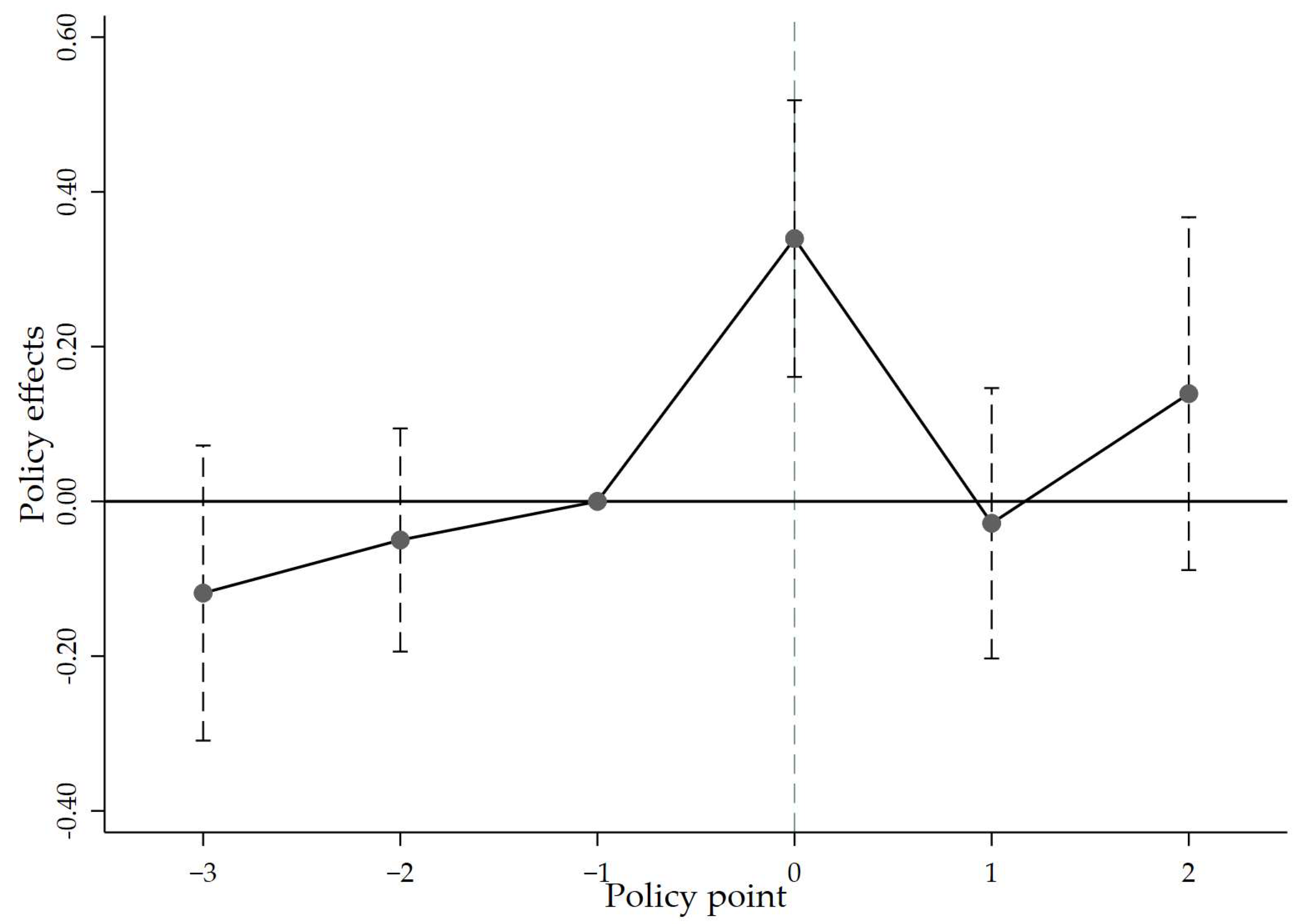
The fundamental premise of the difference-in-differences (DID) methodology is that treated and control provinces exhibit parallel income trajectories prior to the enactment of the policy. To evaluate this hypothesis, this paper adopts the methodology of Bøler et al. (2015) and utilizes an event-study framework to analyze pre-trends. The 2012 wave of CFPS is also used as extra data to make sure there are enough pre-treatment periods for analysis. The specific model is defined as follows:
I n c o m e p i t = a 0 + s 3 2 a s P o l i c y p i t + a 2 X p i t + θ i + λ t + γ p + ε p i t
This specification changes the core explanatory variable from Equation (1) to a group of dummy variables that show the years before and after the agricultural technology extension program was put into place. The implementation year is represented by s = 0, the s-th year before implementation is represented by s < 0, and the s-th year after implementation is represented by s > 0. All other model specifications are in line with Equation (1).
The results of the event-study test for parallel pre-trends are shown in Figure 2. The vertical dashed lines represent 95% confidence intervals, and the year prior to implementation (s = −1) is taken as the baseline period. The findings can be summarized as follows. (i) For all pre-treatment periods (s < −1), the estimated coefficients are statistically insignificant and their confidence intervals encompass zero, indicating no systematic differences in income trends between the treated and control groups before the policy. (ii) A joint significance test of all pre-treatment event-time dummies yields F = 0.48 (p = 0.6194), which fails to reject the null hypothesis of parallel pre-trends. (iii) As an additional robustness check (as can be seen in Table 3), regressions restricted to pre-policy years including covariates are performed. The joint test of covariate–year interactions (F = 1.43, p = 0.2388) also shows no significance, providing further support that the assumption of parallel pre-trends is not violated.
The immediate impact of the policy at the time of implementation can be logically linked to the industrial makeup of the pilot provinces. For instance, Jiangsu focused on seasonal vegetables, Hubei on oilseed rape and horticultural crops, and Sichuan on livestock and vegetable production. All of these have production cycles that are shorter than a year. Zhejiang’s focus on tea, horticulture, medicinal herbs, and flowers also included crops that gave quick returns. These sectoral characteristics elucidate the measurable income increases observed in the inaugural year of policy implementation, primarily fueled by short-cycle crops, aquaculture, and other rapid-return enterprises. On the other hand, it should also be noted that the CFPS data currently extend only to 2022, limiting our ability to capture the longer-run dynamics of the policy impact. With additional post-policy waves, future research may reveal whether the observed short-term response translates into sustained income gains or merely reflects temporary adjustments.
In conclusion, the evidence does not refute the hypothesis of parallel pre-trends between the treated and control groups.

5.1.3. Endogeneity Tests

Even though the baseline regressions show that the agricultural technology extension policy greatly raised household income, possible endogeneity issues can’t be ignored. First, there could be an issue with a missing variable. The model incorporates an extensive array of control variables at various levels to alleviate selection bias; however, it remains challenging to entirely exclude the impact of unobserved factors on the estimates. Second, sample selection bias may occur if pilot and non-pilot regions exhibit systematic differences in either observable or unobservable characteristics, consequently influencing policy identification. To tackle these concerns, this research utilizes robustness checks for omitted variables and a PSM-DID methodology to systematically detect and alleviate potential endogeneity.
  • Test of robustness for omitted variables
This paper employs the ratio method suggested by Altonji et al. (2005) to assess the potential bias introduced by omitted variables in the core estimates. The method evaluates the strength of unobserved factors necessary to invalidate the policy coefficient by comparing a restricted model (Specification A), which incorporates only a subset of controls, with the full model (Specification B), which encompasses all controls. Table 4 shows that when only household, year, and regional fixed effects are included, the ratio compared to the full model is 13.42. This means that variables that were left out would have to be more than 13 times more important than the controls that were included to change the result. The ratio is 953.05 when only regional controls and fixed effects are used. It goes up to 13.12 when only household controls are used. All of the values are much higher than the usual robustness threshold (2), which strongly supports the estimates’ robustness and credibility.
2.
PSM-DID
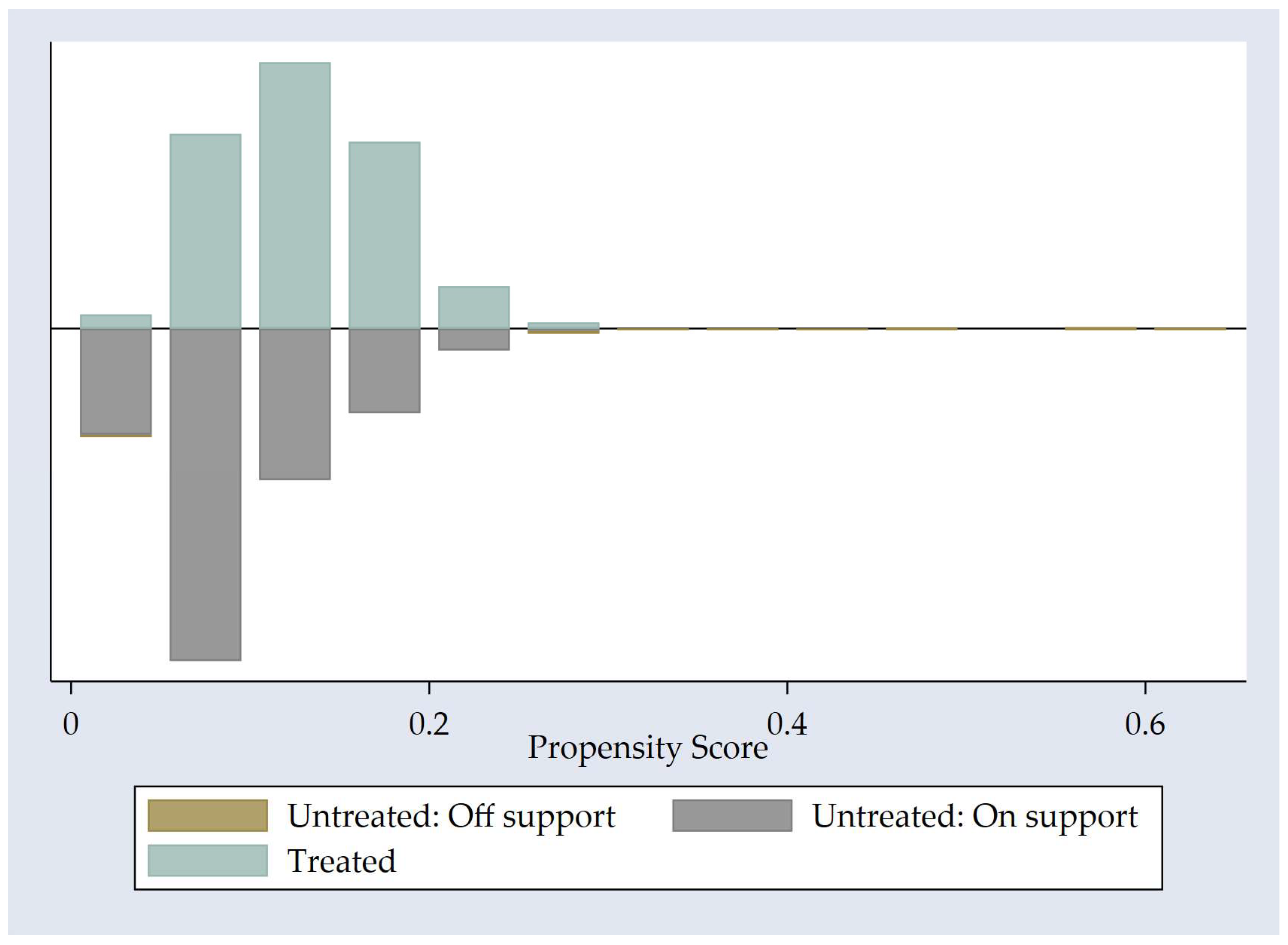
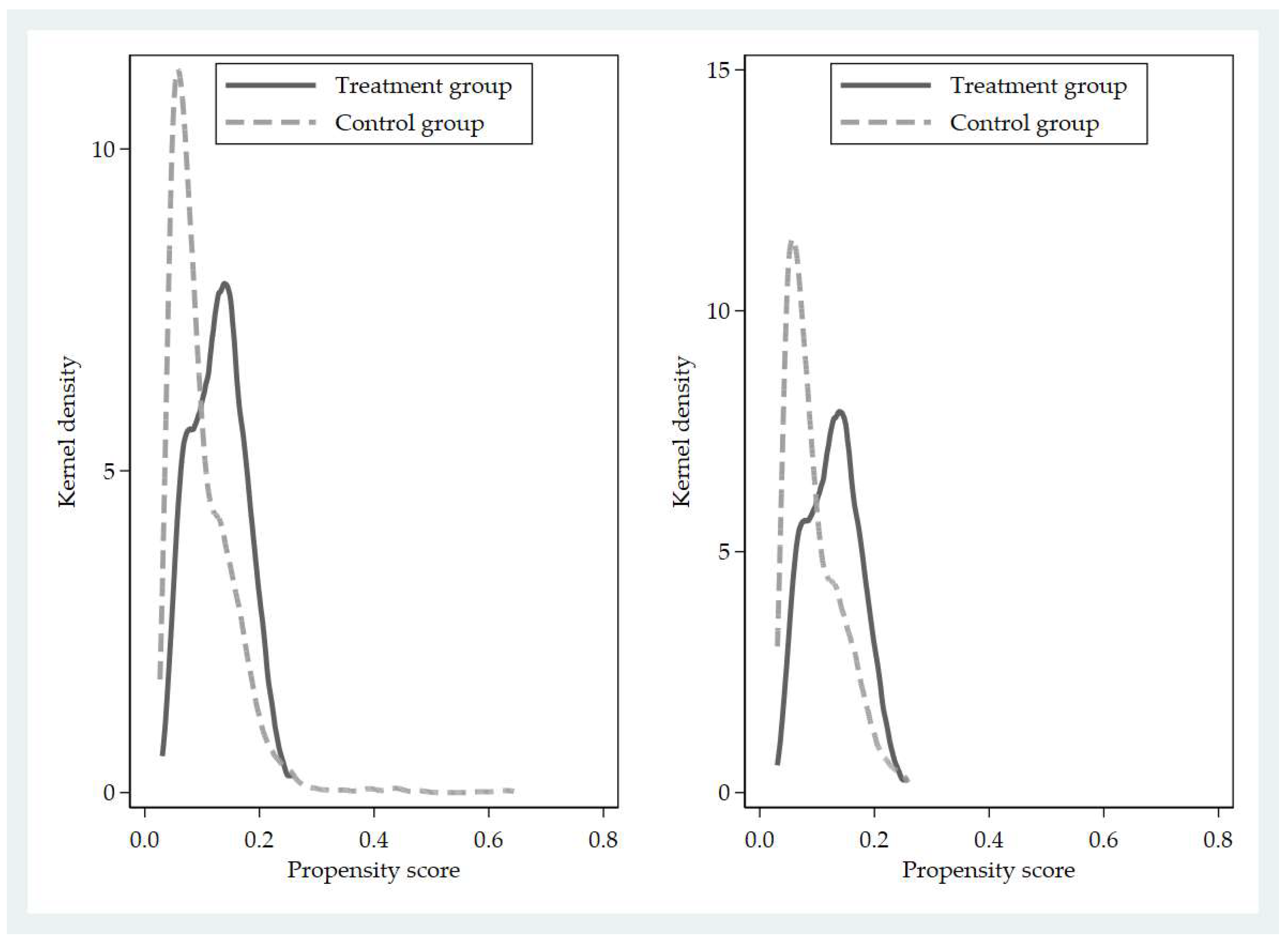
To mitigate potential endogeneity issues stemming from sample selection bias and omitted variables, this study utilizes the propensity score matching difference-in-differences (PSM-DID) methodology as a robustness verification. Table 5 shows that there were significant differences between the treatment and control groups in several covariates before matching. However, after matching, the standardized bias of all covariates (Figure 3) dropped below 10%, and the t-tests were no longer significant. This showed that the balance of the covariates had improved a lot. The propensity score distribution (Figure 4) and kernel density plots (Figure 5) further substantiate that the treatment and control groups demonstrate significant comparability within the common support region.
Table 6 shows the PSM-DID regression results for different matching methods, such as kernel matching (Model 1), caliper matching (radius = 0.01) (Model 2), 1:4 nearest-neighbor matching (with replacement) (Model 3), and nearest-neighbor matching (without replacement) (Model 4). The policy effect (Policy) stays statistically significant in all models, and the estimated coefficients are very close to those from the baseline DID model. This evidence indicates that the findings are not influenced by selection bias but instead demonstrate a strong causal relationship. The PSM-DID analysis bolsters the reliability of the conclusions in accordance with the baseline DID results.

5.1.4. Robustness Test

To confirm the reliability of the baseline results, a series of robustness tests were performed, encompassing placebo tests, outcome variables, winsorization, exclusion of municipalities, and elimination of samples potentially influenced by other exogenous policies.
1.
Placebo tests
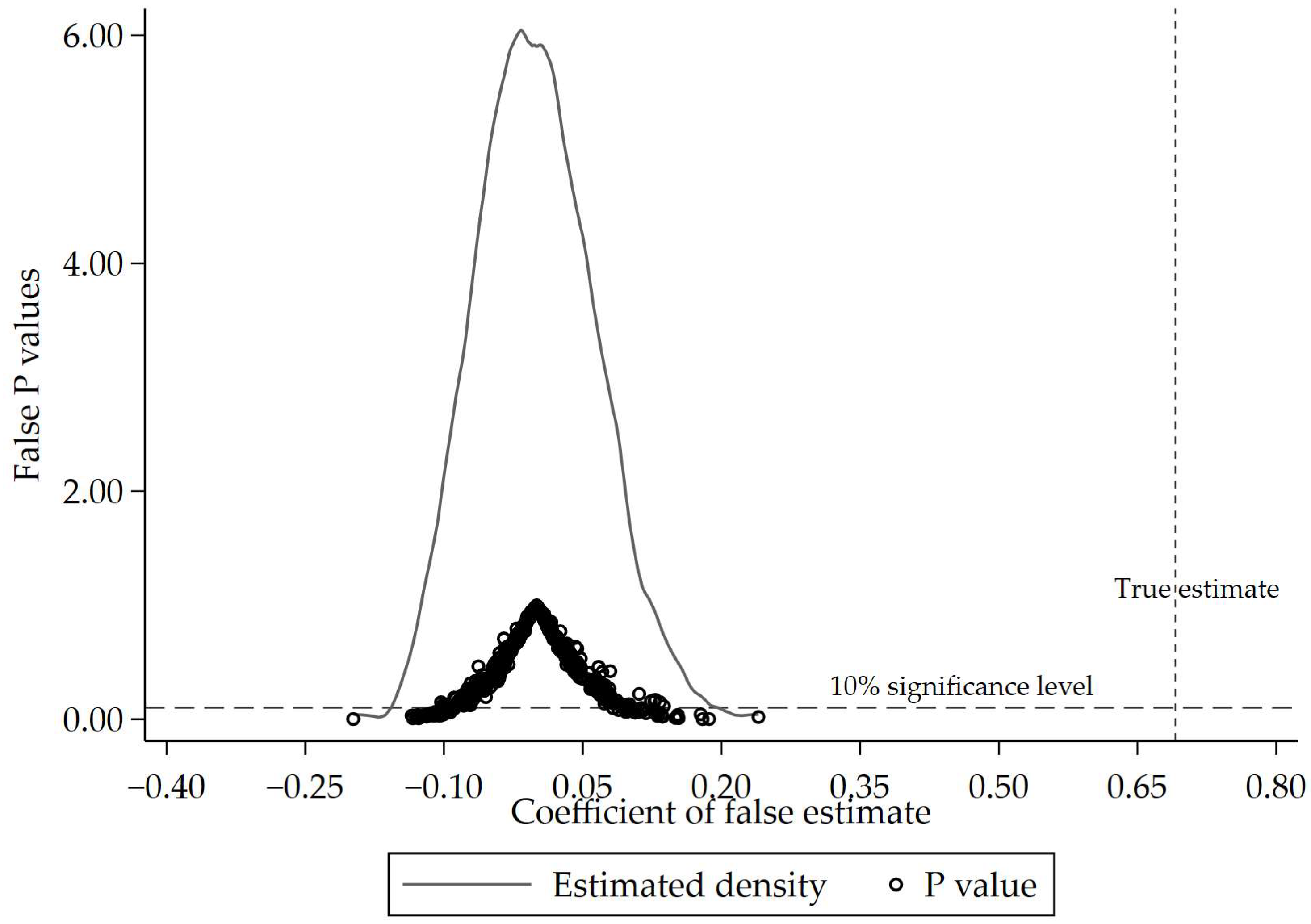
Two types of placebo tests were made to make sure that the baseline estimates were solid. First, in line with Chen et al.’s (2025) method, the year of policy implementation was artificially pushed back to 2016 to create a fake starting point for the policy. All samples that were actually treated from 2018 onward were left out. If the results aren’t affected by pre-trends or other factors that are happening at the same time, the estimated policy effect should get closer to zero. The estimation results (as can be seen in Table 7) in a coefficient of 0.06 with a p-value of 0.62, and the 95% confidence interval encompasses zero, signifying no significant effect of the pseudo-policy. Second, to check for bias that could be caused by confounders that weren’t measured, the treatment variable was randomly given to 500 different groups to create pseudo-treatment groups, and the policy effects were then re-estimated. Figure 6 shows that the placebo coefficients are mostly around zero and have a normal shape. The baseline estimate, on the other hand, is far from the core distribution.
2.
Alternative outcome variable
To mitigate potential bias in income measurement attributable to inflation, household net income was initially deflated using the provincial consumer price index (CPI) of the survey year, subsequently adjusted for household size to derive per capita values, and ultimately converted into natural logarithms (designated as Lincome). The results of the regression (Table 8 Model 1) show that the coefficient of this variable is still significantly positive. This means that the policy’s effect on income stays strong even when price changes are taken into account.
3.
Winsorization
To examine the sensitivity of the baseline estimates to outliers, the dependent variable was winsorized at the top and bottom 1% and 5%, respectively, and the baseline model was re-estimated. Model 2 and 3 of Table 8 report the results. In both specifications, the policy coefficient remains significantly positive at the 1% level, indicating that the income-enhancing effect of the policy is robust to the exclusion of extreme observations.
4.
Excluding municipalities
China’s four municipalities—Beijing, Shanghai, Tianjin, and Chongqing—have higher economic growth and special administrative status. This could make local governments more likely to support agricultural extension services even if they don’t take part in the pilot program, which could change how farmers act. In response to this issue, the baseline model was recalibrated by omitting municipal samples. Model 4 of Table 8 shows that the interaction term of the policy is still significantly positive at the 1% level. This further confirms that the baseline results are strong and trustworthy.
5.
Excluding concurrent policy interventions
In 2019, the National Development and Reform Commission started the National Digital Economy Innovation and Development Pilot Zones in six places: Hebei (Xiong’an New Area), Zhejiang, Fujian, Guangdong, Chongqing, and Sichuan. The goal was to encourage the integration of the digital and real economies. This policy could also have an impact on the income of farm households, so not taking it into account could make it harder to figure out what effect the policy had in this study. The analysis concentrates on samples from Zhejiang, Fujian, Guangdong, Chongqing, and Sichuan, as CFPS does not encompass Xiong’an New Area. We made a policy interaction term (Digi) based on where households lived and when policies were put into place. We then added it to the regression model. The findings, presented in Model 5 of Table 8, further substantiate the income-augmenting impact of agricultural technology extension services.

6. Discussions

6.1. Mechanism Analysis

Based on the preceding theoretical framework, this section empirically examines the mechanisms through which the agricultural technology extension policy affects farm household income.

6.1.1. Production Scale Expansion Pathway

The theoretical framework utilizes two proxy variables at the regional level to evaluate the production expansion mechanism: the provincial land transfer rate (Land) and production input costs (Cost). The outcomes of Model 1 and Model 2 in Table 9 indicate that the policy substantially elevates the provincial land transfer rate (positive coefficient at the 1% level), implying that agricultural technology extension facilitates regional land reallocation and allows more proficient farmers to obtain additional farmland. At the same level, the policy significantly lowers the costs of production inputs (negative coefficient at the 1% level). This means that adopting new technologies makes inputs more efficient and makes it easier to get more money when expanding. In summary, these results show that the collaborative extension program encourages production growth by making land more accessible at the macro level and lowering input costs at the micro level. This expands production boundaries and makes it more appealing for businesses to grow. This evidence shows that agricultural technology extension not only makes production conditions better, but it also makes resource allocation more efficient, which is an important way to increase income.
These findings align with previous research on income-enhancing mechanisms (Danso-Abbeam et al., 2015; Awotide et al., 2016). Awotide et al. (2016) emphasize that technology adoption enhances farmer welfare by increasing yields and market participation, while Danso-Abbeam et al. (2015) highlight that cooperative participation achieves economies of scale through improved resource allocation efficiency. In contrast, the policy mechanism revealed in this study combines both technology diffusion and organizational synergies, forming a systematic transmission pathway from technology adoption to production expansion.

6.1.2. Product Quality Upgrading Pathway

We use the number of organic food certifications (Organic) and the net increase in agro-processing businesses (Process) as mechanism variables to see if the policy raises household income by improving quality. Model 3 and Model 4 in Table 9 show that the policy has a big effect on both the number of organic certifications and the growth of agro-processing businesses. The coefficients are positive at the 1% level. This means that the policy works well to get farmers to use green and environmentally friendly production methods. This makes products safer, increases the number of certifications they can get, and raises the value of their brand, which lets them charge higher prices in the market. The policy also encourages the growth of agro-processing businesses, which adds processing and value-added stages to farming activities. This lengthens the value chain and increases returns. Farmers can get around the problems of only selling raw goods and take advantage of longer value chains, which helps them make more money.
This mechanism is consistent with previous research indicating that farmers can enhance their income by securing price premiums for high-quality products and by distributing value-added returns through the extension of industrial chains (Zhang et al., 2024; Liu et al., 2025). Liu et al. (2025) found that agricultural extension services significantly increased output per unit by enhancing crop technical efficiency, revealing the critical role of knowledge dissemination and service interventions in improving agricultural quality. Meanwhile, Zhang et al. (2024) noted that organic certification and online market access jointly drove up agricultural product prices, demonstrating the synergistic effects of quality signaling and market information mechanisms. In contrast, this study emphasizes a mechanism where coordinated extension policies achieve a systemic transmission pathway from technical efficiency gains to product quality upgrades through the dual effects of technical training and standardized systems.

6.2. Heterogeneity Analysis

This section builds on the mechanism analysis by looking into the different effects of the collaborative extension program on different household characteristics. The goal is to find the factors that affect how the policy affects income.

6.2.1. Household Entrepreneurship

In Model 1, the heterogeneity variable is defined as a binary indicator (Entrepreneurship) that equals 1 if any household member has engaged in self-employment or operated a private business within the past 12 months, and 0 otherwise. Table 10 shows that the policy dummy’s coefficient is positive and statistically significant. This supports the idea that the agricultural technology extension policy generally raises income. The interaction term Policy × Entrepreneurship is more important because it is estimated to be 0.69 and significant at the 5% level. This shows that households with entrepreneurial members get more out of the policy in terms of income growth than households without entrepreneurial members. The finding indicates that entrepreneurial households exhibit heightened market sensitivity and enhanced resource integration capabilities, facilitating their rapid adoption of new technologies, expansion of production networks, and exploration of diversified income streams. This diversity aligns with Schumpeter’s innovation theory, which posits that entrepreneurial spirit, bolstered by institutional frameworks, produces varied economic outcomes via innovation and market restructuring.

6.2.2. Household Financial Assets

In Model 2, the heterogeneity variable is quantified by the logarithm of the household’s total financial assets (Financial assets). The policy coefficient stays positive and very important, which again shows that the agricultural technology extension policy helps farmers make more money. The interaction term Policy × Financial assets, on the other hand, is negative and significant at the 5% level. This indicates that the marginal income effect of the policy diminishes as households’ financial assets rise. This outcome can be elucidated through the capital constraint hypothesis: households with diminished financial capital face greater limitations in the adoption of agricultural technologies, and the policy is instrumental in alleviating these constraints and lowering trial costs. On the other hand, households that already have a lot of money are more liquid and better able to protect themselves against risk, so the policy doesn’t have as big of an effect on their income. This diversity shows that agricultural extension policies can help households that don’t have a lot of money more than others.
Lastly, the results show that different groups are affected in very different ways by the agricultural technology extension policy. Households engaged in entrepreneurship receive greater benefits, indicating a disparity influenced by market participation and organizational capacity. On the other hand, the income effects get less significant as financial assets increase, which shows that there is a variance based on capital endowments and financial limits. These results show that agricultural technology extension policies don’t work the same way for all households. Instead, they work differently depending on the characteristics of each household.

6.3. The Spillover Effects

This study utilizes the DID method to ascertain the average treatment effect of the MATCEP within the framework of the baseline model previously presented. To further analyze the policy’s geospatial spillover effects, in accordance with Cao (2020) and Wang and Bu (2019), we incorporate interaction terms categorized by spatial distance into Equation (6), defined as follows:
I n c o m e p k t = α 0 + α 1 D D D p k t + s = 0 2000 δ s N p k t s + α 2 X p k t + λ t + γ p + ε p k t
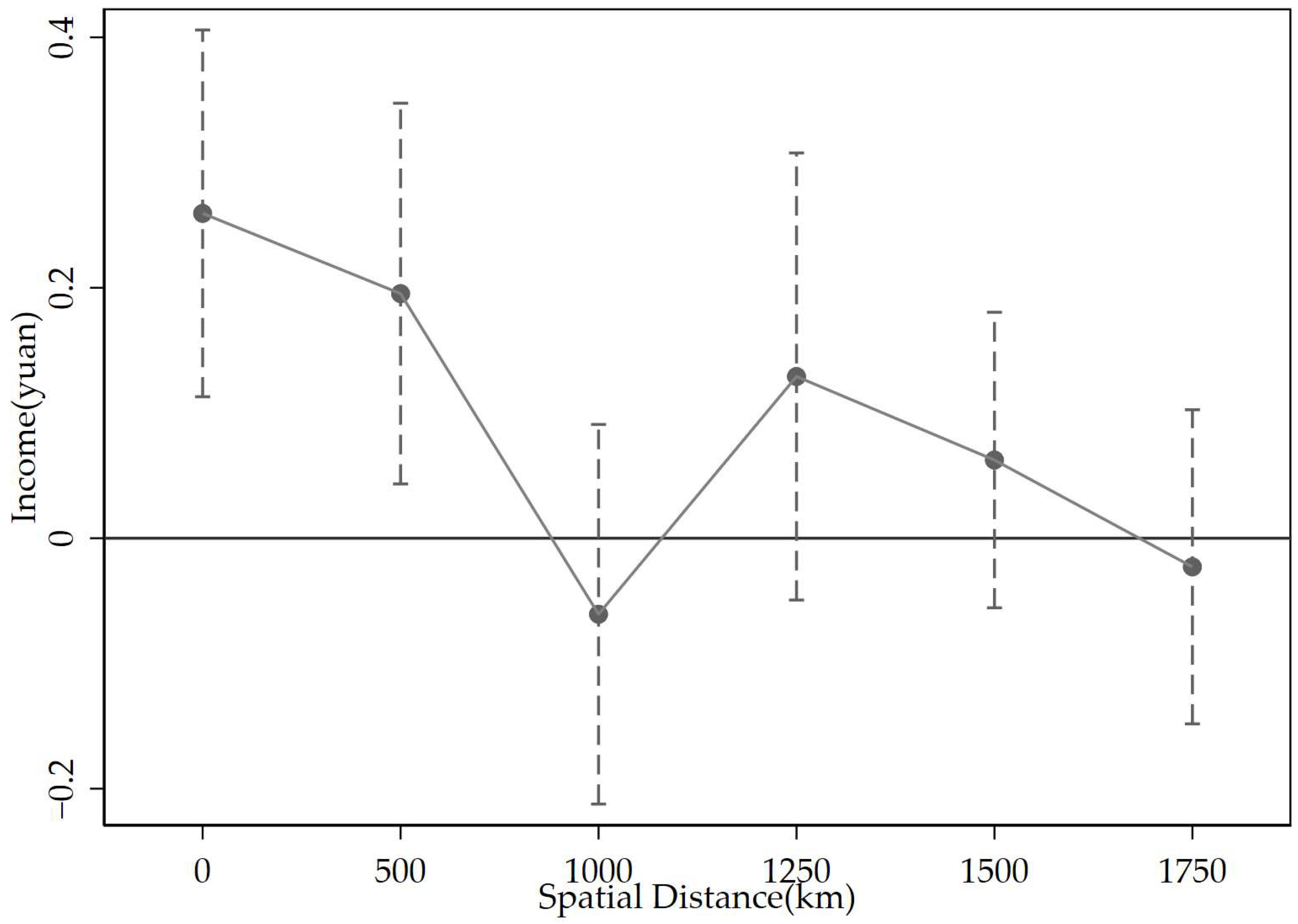
In this case,  N p k t s  shows whether there is a policy pilot province within s kilometers of province p in year t (1 if there is one, 0 if there isn’t). The spatial distance is measured using the great-circle distance between provincial capitals. This study employs a 250-km increment, sequentially setting s = 0, 250, 500, 750, 1000, 1250, 1500, 1750 and 2000 km. It identifies the spatial transmission patterns of policy effects by comparing the estimated values and significance levels of  δ s  at various distances. In contrast to Cao (2020)’s city-level analysis, this study utilizes provinces as the analytical unit and employs the great circle distance between provincial geographic centers for spatial measurement, thereby elucidating the diffusion characteristics of policies at the interprovincial level.
Figure 7 plots the spatial variation of  N p k t s  based on Equation (6) (with a 95% confidence interval). Specifically, MTACEP has a spillover effect on income in nearby provinces. First, when s = 0, agricultural technology extension leads to substantial income increases for the pilot province, aligning with the benchmark regression findings and reinforcing Hypothesis 1. Second, agricultural technology extension has income-boosting effects that reach neighboring provinces up to 1000 km away. These effects start to fade after 1000 km and stay that way after that. This means that the policy’s spatial spillover effects are limited to certain areas, mostly those that are close by and have stronger agricultural and extension network connections. This shows that the policy’s spatial spillover effects have clear geographical limits, mostly in nearby areas with similar agricultural structures, resource endowments, and extension networks. These limitations may be due to things like the limited spread of technical knowledge and demonstration effects, as well as restrictions on the movement of extension workers and agricultural capital between regions. As a result, the policy’s effects are mostly limited to areas that are close to each other.

6.4. Global Perspective

As discussed in Section 3.1. (Policy Background), the implementation of China’s MATCEP is closely linked to its unique institutional and developmental context. To better understand its structural features and policy logic, it is instructive to place MATCEP within the broader global evolution of agricultural extension systems. Across countries, diverse institutional arrangements have emerged to address similar challenges of technological diffusion, fiscal constraints, and farmer participation. In high-income economies, agricultural extension has become institutionalized and professionalized through law-based and multi-level governance frameworks that ensure stable public financing, decentralized accountability, and strong knowledge linkages among universities, research institutes, and farm service systems. In contrast, many developing economies operate state-dominated or donor-dependent systems marked by centralized administration, fiscal volatility, and weak integration between research and field practice, which often constrain technological diffusion and long-term sustainability. The following cross-country comparison examines these representative institutional configurations to position China’s MATCEP within the broader global spectrum of extension governance and innovation models.
In high-income economies, institutionalized and law-based dual-track models predominate. Japan operates a vertically integrated government–cooperative system in which the Ministry of Agriculture coordinates prefectural improvement centers while agricultural cooperatives deliver ”pre-production to post-harvest” services covering over 90 percent of farm households. The United States exemplifies the education–research–extension triad codified in the Smith–Lever Act (1914): Land-Grant Universities and the USDA jointly fund roughly 2900 county extension offices, achieving a technology-transfer rate exceeding 80 percent and demonstrating the capacity of higher-education institutions to couple scientific innovation with large-scale diffusion.
Among developing economies, Thailand’s high-density, donor-supported network—co-financed by the World Bank and the Ministry of Agriculture—illustrates how external assistance and state coordination can jointly build extensive outreach (one agent per 1000 farmers) and integrate export-oriented value-chain services such as durian varietal improvement and cold-chain logistics. The Philippines follows a high-human-capital public system, legislated through its Agricultural Extension Act, yet faces fiscal and geographic constraints owing to archipelagic dispersion. Malaysia’s commodity-board model, led by the Rubber Board and crop-specific associations, provides end-to-end technical and marketing services for cash crops, whereas the United Kingdom and France rely heavily on private firms whose agronomic advice is intertwined with agro-input sales, raising debates on the balance between commercial and public-interest objectives.
In Latin America, Brazil’s PNATER policy (2004, 2010) institutionalized a pluralistic and participatory approach, linking public agencies, cooperatives, and NGOs to support family farming and agro-ecological practices, while Colombia’s AgroSavia network demonstrates the territorial innovation model that connects research centers with producer associations. Across Sub-Saharan Africa, Uganda’s NAADS → SSES reform and Ethiopia’s large-scale public system of Farmers Training Centers (FTCs) exemplify divergent paths: Uganda’s market-oriented but fiscally constrained demand-driven framework versus Ethiopia’s state-financed, high-coverage but standardized supply model. Malawi and the Democratic Republic of Congo further reveal the post-aid transition challenge—limited operational funding, weak coordination, and human-resource bottlenecks undermine service continuity despite extensive donor involvement.
Table 11 shows how agricultural technology extension systems differ from country to country and how their institutional forms change over time. In mature systems, the way that governance, financing, service delivery, and knowledge networks operate together usually decides how well new technology get to farmers (Birner et al., 2009; Anderson & Feder, 2007; Davis, 2008; Klerkx & Leeuwis, 2009; Spielman et al., 2008). Countries with clear lines of duty and local agents who can act flexibly within national frameworks frequently do a good job of keeping both accountability and innovation alive. On the financing side, steady but varied funding sources, which sometimes include local governments and producer groups, have been very important for keeping extension activities going beyond brief policy cycles. Service delivery involves more than just coordinating administrative tasks. It also includes how extension staff talk to farmers, how feedback loops work, and how success is judged in real-life situations. The final dimension, knowledge linkage, hinges on the ability of researchers, firms, and producers to interact rather than operate in parallel; this influences the transition of breakthroughs from laboratories to practical applications.
From this point of view, China’s Major Agricultural technological Collaborative Extension Program (MATCEP) is a unique attempt to close the “last mile” of technological dissemination. It works well because the government works well with colleges, agribusinesses, and cooperatives. The program doesn’t just rely on top-down management. Instead, it encourages central and local levels to work together to fund initiatives, test ideas in the field, and promote learning and flexibility through peer-based assessments. These tools help make the extension system more responsive and able to improve itself. MATCEP is different from many other donor-driven programs in that it works within a long-term institutional framework that includes extension in the larger innovation ecosystem. This makes it a good model for other developing economies that want to find a balance between state leadership and local initiative and knowledge-based collaboration.

7. Research Conclusions and Policy Implications

This study draws upon the 2018 initiation of the Major Agricultural Technology Collaborative Extension Program as a quasi-natural experiment, alongside five waves of CFPS data (2014–2022), employing a difference-in-differences (DID) model integrated with mechanism and heterogeneity analyses. The primary conclusions are as follows.
The policy first and foremost raised the income of farm families by a lot. According to baseline estimates, per capita net income in the pilot regions went up by about 24.71%. This effect stays strong even when we do a lot of robustness tests. This shows that the collaborative extension program really did turn agricultural technological achievements into real income gains.
Second, the policy works through two pathways: increasing the scale of production and improving the quality of the products. Tests of the policy’s effects show that it increased the rate of land transfers, lowered the costs of production inputs, increased the number of organic food certifications, and encouraged the growth of agro-processing businesses. These results indicate that the program not only improves economies of scale by promoting land consolidation and organized production, but also enhances product competitiveness through certification and value chain extension, resulting in income growth in both quantity and quality.
Third, the effects are different for each household. Households with entrepreneurial members benefit more because they are more market-oriented and better at integrating resources. On the other hand, households with fewer financial assets see bigger marginal gains. This shows that agricultural extension works with household characteristics to improve both efficiency and fairness.
In summary, the collaborative extension program enhances farm household income on average, functions through various mechanisms, and demonstrates diverse effects among household groups, highlighting the intricacies of policy dissemination. These results offer novel empirical evidence to inform the enhancement of extension policies.
The implications for the policy are clear. Policymakers should: (i) consolidate and expand extension programs as institutionalized channels for income growth, ensuring that technological achievements are effectively translated into sustained household welfare improvements; (ii) reinforce both production scale expansion and product quality upgrading by promoting land transfer, cooperative arrangements, and factor market reforms on the one hand, and linking extension with certification systems, branding, and agro-processing industries on the other; and (iii) tailor extension strategies to household heterogeneity by integrating entrepreneurship training and rural innovation initiatives for market-oriented households, while expanding inclusive rural finance and credit programs to enable financially constrained households to fully benefit from technology diffusion.
While these findings offer valuable lessons for other developing economies, their broader applicability depends on several institutional prerequisites. Successful implementation of collaborative extension programs requires strong government coordination capacity, well-established agricultural data and monitoring systems, and reliable channels for linking research institutions with grassroots extension agents. Therefore, the results should be viewed not as a blueprint for direct replication, but as evidence-based insights illustrating how coordinated technological extension and institutional support can jointly enhance rural income growth under China’s unique administrative context.
This study still has several limitations. First, at the data level, the CFPS data used in this research only extends to 2022, reflecting the implementation outcomes of the first batch of pilot projects under the Major Agricultural Technology Collaborative Extension Program (MATCEP). Since the policy launched its second batch of extensions in 2023 but relevant microdata has not yet been released, it is impossible to further examine the policy’s sustainability and diffusion effects in subsequent phases. This constitutes a significant limitation of this paper. Second, regarding heterogeneity analysis, as a household-based longitudinal survey, CFPS has limited coverage of agricultural production activities, input structures, and crop types. This hinders the study’s ability to reveal nuanced production-level differences in how various farmer types respond to technology promotion, thereby limiting the depth of mechanism analysis. Finally, as a provincial-level pilot policy, MATCEP’s identification precision is constrained by variations in provincial policy implementation and internal heterogeneity. It struggles to fully capture execution differences at the county or grassroots levels, thereby affecting the accuracy of policy effect estimates to some extent. Future research could conduct more in-depth evaluations of the policy’s long-term impacts by integrating the latest CFPS data with supplementary datasets containing richer agricultural and enterprise-level information.

Author Contributions

Conceptualization, F.L. and X.P.; methodology, Y.L. and X.P.; software, X.P.; validation, X.P.; formal analysis, Y.L. and X.P.; investigation, X.P.; resources, F.L.; data curation, X.P.; writing—original draft preparation, F.L. and X.P.; writing—review and editing, F.L., Y.L. and J.W.; visualization, X.P.; supervision, F.L. and Y.L.; project administration, F.L. All authors have read and agreed to the published version of the manuscript.

Funding

This paper was supported by the National Social Science Fund of China (General Project) (Project No. 25BJL037, “Research on the Micro-Mechanisms and Implementation Paths of the Digital Transformation of Non-Scale Agricultural Production Services”), the Ministry of Education Humanities and Social Sciences Research General Project of China (Project No. 23YJA790040, “Research on the Income-Increasing Mechanisms and Effects of Smallholder Cooperative Operations”), and the Yunnan Provincial Philosophy and Social Science Fund General Project (Project No. YB2021023, “Research on the Ideas, Goals, and Measures for the Digital Transformation of Agriculture in Yunnan Province”), all of which were funded under the supervision of F.L.; and by the National Natural Science Foundation of China (NSFC) (Project No. 72063035, “Field Experimental Research on the Competition Game of the Impact of Digital Inequality on Belief Bias, Competitive Willingness and Income”), funded under the supervision of Y.L.

Institutional Review Board Statement

Not applicable.

Data Availability Statement

The data were obtained from the China Family Panel Studies (CFPS), which are administered by the Institute of Social Science Survey (ISSS) of Peking University. CFPS data are available upon application at https://opendata.pku.edu.cn/ (accessed on 7 November 2025) with the permission of ISSS.

Conflicts of Interest

The authors declare no conflicts of interest.

Abbreviations

The following abbreviations are used in this manuscript:
MATCEPMajor Agricultural Technology Collaborative Extension Program
CFPSChina Family Panel Studies
DIDDifference-in-Differences
FEsFixed Effects

Appendix A

Appendix A.1. Robustness Tests for Adjusting the Clustering Level

To further verify the robustness of the baseline results and considering that the MATCEP is a provincial-level pilot policy, we adjust the clustering level of standard errors to both the province and village levels. Models (1) and (2) in Table A2 report the regression results clustered at the province and village levels, respectively. Compared with the baseline regression, the estimated policy effect remains positive and statistically significant when clustering at the provincial level, indicating that the results are not driven by intra-provincial correlations. When clustering at the village level, the magnitude of the policy effect slightly increases and remains significant at the 1% level. These findings demonstrate that the income-enhancing effect of MATCEP is robust across different clustering levels, further strengthening the credibility of the results. Moreover, a wild cluster bootstrap-t procedure clustered at the provincial level (Figure A1) yields consistent results, confirming that the policy effect remains robust even under a small number of clusters.
Table A1. Robustness Tests for Adjusting the Clustering Level.
VariablesModel 1Model 2
Clustered at the Province LevelClustered at the Village Level
Policy0.2471 **0.2688 ***
(0.0890)(0.0968)
Consumption−0.2303 ***−0.2310 *
(0.0750)(0.1282)
School−0.1980 *−0.1928 *
(0.1093)(0.1085)
Library0.06280.0673
(0.0478)(0.0740)
Phone−0.0614−0.0696
(0.2215)(0.2071)
Education0.00590.0071
(0.0093)(0.0212)
Health0.01110.0111
(0.0149)(0.0159)
Cons4.9972 ***5.0043 ***
(1.4613)(1.8819)
Individual FEsYESYES
Year FEsYESYES
Region FEsYESYES
R 2 0.57350.5811
N78237765
In this table, *, **, and *** denote statistical significance at the 10%, 5%, and 1% levels, respectively. Robust standard errors clustered at the household level are reported in parentheses.
Figure A1. Wild Cluster Bootstrap-t Confidence Interval for the Policy Effect. This figure illustrates the wild cluster bootstrap-t confidence interval for the estimated policy coefficient, obtained following the procedure of Cameron et al. (2008). The test is based on 999 bootstrap replications clustered at the provincial level. The horizontal axis represents alternative hypothesized values of the policy effect, while the vertical axis reports the corresponding bootstrap p-values. The sharp peak indicates the coefficient value most consistent with the sample data, where the null hypothesis cannot be rejected. The two gray diamonds denote the 95% confidence interval [0.053, 0.556], confirming that the positive income effect of the MATCEP remains statistically significant (t = 2.27, p = 0.025) and robust to the small number of clusters.
Economies 13 00331 g0a1

Appendix A.2. Robustness Test for Controlling Provincial-Specific Time Trends

To address potential biases arising from region-specific shocks that vary over time, this study extends the baseline model by incorporating province-specific linear time trends—specifically, by adding interaction terms between provinces and time. This specification allows provinces to exhibit distinct income growth trajectories over the sample period, thereby controlling for systematic biases stemming from variations in regional economic development paths, infrastructure development, rural financial expansion, or agricultural subsidy intensity.
Empirical results are presented in Table A1. After incorporating province-specific linear time trends, the regression coefficient for the policy variable (Policy) remains significantly positive, indicating robust income-promoting effects of the Major Agricultural Technology Cooperative Extension Program. Even after controlling for linear trend factors like provincial economic growth rates, public investment, and agricultural input policies, the policy implementation significantly boosted farmer incomes. This indicates that the policy effect is not driven by long-term provincial development trends but stems from the policy’s direct promotion of agricultural productivity and farmer earnings.
Simultaneously, the coefficients for the time trend term in some provinces were significantly positive, indicating faster income growth trajectories in these regions during the sample period. Conversely, coefficients in other provinces were insignificant or negative, reflecting divergent income growth paths across regions. This corroborates the reviewers’ observation regarding “asynchronous regional economic development.” Overall, controlling for province-specific time trends maintains the robustness of the policy effects, further strengthening the causal explanatory power of this paper’s conclusions.
Table A2. Robustness Test for Controlling Provincial-Specific Time Trends.
VariablesIncome
Policy0.3838 **
(0.1531)
Consumption−0.3317 ***
(0.1154)
School−0.1753 *
(0.0922)
Library0.0325
(0.0596)
Phone−0.0424
(0.1437)
Education0.0085
(0.0162)
Health0.0109
(0.0140)
Cons0.0613
(0.1188)
12.province × Year−0.0027
(0.0168)
13.province × Year−0.0148
(0.0200)
14.province × Year0.0123
(0.0199)
21.province × Year−0.0624
(0.0516)
22.province × Year0.0252
(0.0265)
23.province × Year0.1954 ***
(0.0184)
31.province × Year0.0104
(0.0708)
32.province × Year0.1844 *
(0.1047)
33.province × Year0.1820 *
(0.1027)
34.province × Year0.1406
(0.0933)
35.province × Year−0.0180
(0.0378)
36.province × Year0.0809 ***
(0.0251)
37.province × Year0.0280 *
(0.0158)
41.province × Year0.0198
(0.0553)
42.province × Year0.0060
(0.1049)
43.province × Year0.0426 *
(0.0243)
44.province × Year−0.0280
(0.0383)
45.province × Year−0.0050
(0.0392)
50.province × Year−0.0171
(0.0428)
51.province × Year−0.0160
(0.0718)
52.province × Year0.0341
(0.0341)
53.province × Year0.0093
(0.0197)
61.province × Year6.6380 ***
(1.9279)
Individual FEsYES
Year FEsYES
Region FEsYES
R 2 0.5777
N7823
In this table, *, **, and *** denote statistical significance at the 10%, 5%, and 1% levels, respectively. Robust standard errors clustered at the household level are reported in parentheses.

References

  1. Abay, K. A. (2017). Estimating input complementarities with unobserved heterogeneity: Evidence from Ethiopia. Journal of Agricultural Economics, 68(2), 518–541. [Google Scholar] [CrossRef]
  2. Addai, K. N., Temoso, O., & Ng’ombe, J. N. (2023). Heterogeneous effects of agricultural technology adoption on smallholder household welfare in Ghana. Journal of Agricultural and Applied Economics, 55(2), 283–303. [Google Scholar] [CrossRef]
  3. Akzar, R., Umberger, W. J., & Peralta, A. (2022). Understanding heterogeneity in technology adoption among Indonesian smallholder dairy farmers. Agribusiness, 38(4), 899–918. [Google Scholar] [CrossRef]
  4. Altonji, J. G., Elder, T. E., & Taber, C. R. (2005). Selection on observed and unobserved variables: Assessing the effectiveness of Catholic schools. Journal of Political Economy, 113(1), 151–184. [Google Scholar] [CrossRef]
  5. Anderson, J. R., & Feder, G. (2004). Agricultural extension: Good intentions and hard realities. The World Bank Research Observer, 19(1), 41–60. [Google Scholar] [CrossRef]
  6. Anderson, J. R., & Feder, G. (2007). Agricultural extension. In R. Evenson, & P. Pingali (Eds.), Handbook of agricultural economics (Vol. 3, pp. 2343–2378). Elsevier. [Google Scholar] [CrossRef]
  7. Awotide, B. A., Karimov, A. A., & Diagne, A. (2016). Agricultural technology adoption, commercialization and smallholder rice farmers’ welfare in rural Nigeria. Agricultural and Food Economics, 4(1), 3. [Google Scholar] [CrossRef]
  8. Baron, R. M., & Kenny, D. A. (1986). The moderator–mediator variable distinction in social psychological research: Conceptual, strategic, and statistical considerations. Journal of Personality and Social Psychology, 51(6), 1173–1182. [Google Scholar] [CrossRef]
  9. Barrett, C. B., & Carter, M. R. (2013). The economics of poverty traps and persistent poverty: Empirical and policy implications. Journal of Development Studies, 49(7), 976–990. [Google Scholar] [CrossRef]
  10. Barrett, C. B., Reardon, T., & Webb, P. (2001). Nonfarm income diversification and household livelihood strategies in rural Africa: Concepts, dynamics, and policy implications. Food Policy, 26(4), 315–331. [Google Scholar] [CrossRef]
  11. Becerra-Encinales, J. F., Bernal-Hernandez, P., Beltrán-Giraldo, J. A., Cooman, A. P., Reyes, L. H., & Cruz, J. C. (2024). Agricultural extension for adopting technological practices in developing countries: A scoping review of barriers and dimensions. Sustainability, 16(9), 3555. [Google Scholar] [CrossRef]
  12. Bernoulli, D. (1954). Exposition of a new theory on the measurement of risk. Econometrica, 22(1), 23–36, (Original work published 1738). [Google Scholar] [CrossRef]
  13. Birner, R., Davis, K., Pender, J., Nkonya, E., Anandajayasekeram, P., Ekboir, J., Mbabu, A., Spielman, D. J., Horna, D., Benin, S., & Cohen, M. (2009). From best practice to best fit: A framework for designing and analyzing pluralistic agricultural advisory services. Journal of Agricultural Education and Extension, 15(4), 341–355. [Google Scholar] [CrossRef]
  14. Bøler, E. A., Moxnes, A., & Ulltveit-Moe, K. H. (2015). R&D, international sourcing, and the joint impact on firm performance. American Economic Review, 105(12), 3704–3739. [Google Scholar] [CrossRef]
  15. Cameron, A. C., Gelbach, J. B., & Miller, D. L. (2008). Bootstrap-based improvements for inference with clustered errors. The Review of Economics and Statistics, 90(3), 414–427. [Google Scholar] [CrossRef]
  16. Cao, Q. (2020). The driving effect of national new areas on regional economic growth: Empirical evidence from 70 large and medium-sized cities. China Industrial Economy, 2020(7), 43–60. [Google Scholar] [CrossRef]
  17. Carter, M. R., & Barrett, C. B. (2006). The economics of poverty traps and persistent poverty: An asset-based approach. Journal of Development Studies, 42(2), 178–199. [Google Scholar] [CrossRef]
  18. Chen, Q., Qi, J., & Yan, G. (2025). A practical guide to placebo tests in difference-in-differences method. Management World, 41(2), 181–220. [Google Scholar] [CrossRef]
  19. Coase, R. H. (1960). The problem of social cost. Journal of Law and Economics, 3(1), 1–44. [Google Scholar] [CrossRef]
  20. Dai, Z., Wang, Q., Jiang, J., & Lu, Y. (2024). Influence of university agricultural technology extension on efficient and sustainable agriculture. Scientific Reports, 14(1), 4874. [Google Scholar] [CrossRef]
  21. Danso-Abbeam, G., Dahamani, A. M., & Bawa, G. A. S. (2015). Resource-use efficiency among smallholder groundnut farmers in Northern Region, Ghana. American Journal of Experimental Agriculture, 6(5), 290–304. [Google Scholar] [CrossRef]
  22. Davis, K. E. (2008). Extension in sub-Saharan Africa: Overview and assessment of past and current models, and future prospects. Journal of International Agricultural and Extension Education, 15(3), 15–28. Available online: https://drive.google.com/file/d/1hnw7mOLw_r-8zv5u3NnRyUOZ6yvhM0Zx/view (accessed on 10 November 2025).
  23. Dinar, A., Karagiannis, G., & Tzouvelekas, V. (2007). Evaluating the impact of agricultural extension on farms’ performance in Crete: A nonneutral stochastic frontier approach. Agricultural Economics, 36(2), 135–146. [Google Scholar] [CrossRef]
  24. Feder, G., Just, R. E., & Zilberman, D. (1985). Adoption of agricultural innovations in developing countries: A survey. Economic Development and Cultural Change, 33(2), 255–298. [Google Scholar] [CrossRef]
  25. Haggblade, S., Hazell, P. B. R., & Reardon, T. (2010). The rural non-farm economy: Prospects for growth and poverty reduction. World Development, 38(10), 1429–1441. [Google Scholar] [CrossRef]
  26. Huang, Z. (2014). Is ‘family farms’ the way to develop Chinese agriculture? Rural China, 11(2), 189–221. Available online: https://brill.com/view/journals/rchs/11/2/article-p189_1.xml (accessed on 10 November 2025).
  27. Kissoly, L., Faße, A., & Grote, U. (2017). The integration of smallholders in agricultural value chain activities and food security: Evidence from rural Tanzania. Food Security, 9(6), 1219–1235. [Google Scholar] [CrossRef]
  28. Klerkx, L., & Leeuwis, C. (2009). Establishment and embedding of innovation brokers at different innovation system levels: Insights from the Dutch agricultural sector. Technological Forecasting and Social Change, 76(6), 849–860. [Google Scholar] [CrossRef]
  29. Krishnan, P., & Patnam, M. (2014). Neighbors and extension agents in Ethiopia: Who matters more for technology adoption? American Journal of Agricultural Economics, 96(1), 308–327. [Google Scholar] [CrossRef]
  30. Liu, C., Li, W., You, Y., Yang, Q., & Li, M. (2025). Research on leading agricultural enterprises guiding farmers’ participation in pre-production quality and safety control: Evidence from the Yangtze River Delta Region of China. Frontiers in Sustainable Food Systems, 9, 1615223. [Google Scholar] [CrossRef]
  31. Markowitz, H. (1952). Portfolio selection. Journal of Finance, 7(1), 77–91. [Google Scholar] [CrossRef]
  32. Martini, E., Pagella, T., Mollee, E., & van Noordwijk, M. (2023). Relational values in locally adaptive farmer-to-farmer extension: How important? Current Opinion in Environmental Sustainability, 65, 101363. [Google Scholar] [CrossRef]
  33. Mathenge, M. K., Smale, M., & Olwande, J. (2014). The impacts of hybrid maize seed on the welfare of farming households in Kenya. Food Policy, 44, 262–271. [Google Scholar] [CrossRef]
  34. Meemken, E. M. (2020). Do smallholder farmers benefit from sustainability standards? A systematic review and meta-analysis. Global Food Security, 26, 100373. [Google Scholar] [CrossRef]
  35. Michalscheck, M., Ekpe, S., Birhanu, B. Z., Traore, A., Keita, M., & Giller, K. E. (2024). An evaluative framework for inclusive agricultural value chain policies and interventions—Case: Mali. Global Food Security, 42, 100769. [Google Scholar] [CrossRef]
  36. Norton, G. W., & Alwang, J. (2020). Changes in agricultural extension and implications for farmer adoption of new practices. Applied Economic Perspectives and Policy, 42(1), 8–20. [Google Scholar] [CrossRef]
  37. Oyetunde-Usman, Z. (2022). Heterogeneous factors of adoption of agricultural technologies in West and East Africa countries: A review. Frontiers in Sustainable Food Systems, 6, 761498. [Google Scholar] [CrossRef]
  38. Oyetunde-Usman, Z., & Shee, A. (2023). Adoption of drought-tolerant maize varieties and interrelated climate-smart agricultural practices in Nigeria. Agriculture & Food Security, 12, 43. [Google Scholar] [CrossRef]
  39. Pitawala, D. (2024). Entrepreneurial behavior, technology adoption, and climate change resilience: Evidence from small and medium-scale livestock and maple producers in Vermont. The University of Vermont and State Agricultural College. Available online: https://scholarworks.uvm.edu/graddis/1933 (accessed on 7 November 2025).
  40. Prahladachar, M. (1983). Income distribution effects of the green revolution in India: A review of empirical evidence. World Development, 11(11), 927–944. [Google Scholar] [CrossRef]
  41. Pratt, J. W. (1964). Risk aversion in the small and in the large. Econometrica, 32(1/2), 122–136. [Google Scholar] [CrossRef]
  42. Qiao, D., Li, N., Cao, L., Zhang, D., Zheng, Y., & Xu, T. (2022). How agricultural extension services improve farmers’ organic fertilizer use in China? The perspective of neighborhood effect and ecological cognition. Sustainability, 14(12), 7166. [Google Scholar] [CrossRef]
  43. Rahman, M. M., & Connor, J. D. (2022). Impact of agricultural extension services on fertilizer use and farmers’ welfare: Evidence from Bangladesh. Sustainability, 14(15), 9385. [Google Scholar] [CrossRef]
  44. Schumpeter, J. A. (1934). The theory of economic development: An inquiry into profits, capital, credit, interest, and the business cycle. Harvard University Press. [Google Scholar]
  45. Sellare, J., Meemken, E. M., Kouamé, C., & Qaim, M. (2020). Do sustainability standards benefit smallholder farmers also when accounting for cooperative effects? Evidence from Côte d’Ivoire. American Journal of Agricultural Economics, 102(2), 681–695. [Google Scholar] [CrossRef]
  46. Spence, M. (1973). Job market signaling. Quarterly Journal of Economics, 87(3), 355–374. [Google Scholar] [CrossRef]
  47. Spielman, D. J., Ekboir, J., Davis, K., & Ochieng, C. M. O. (2008). An innovation systems perspective on strengthening agricultural education and training in sub-Saharan Africa. Agricultural Systems, 98(1), 1–9. [Google Scholar] [CrossRef]
  48. Takahashi, K., Muraoka, R., & Otsuka, K. (2020). Technology adoption, impact, and extension in developing countries’ agriculture: A review of the recent literature. Agricultural Economics, 51(1), 31–45. [Google Scholar] [CrossRef]
  49. Wang, X., & Bu, L. (2019). International export trade and enterprise innovation—A Quasi-natural experimental study based on the opening of the “China-Europe Freight Train”. China Industrial Economy, 10, 80–98. [Google Scholar] [CrossRef]
  50. Ward, P. S., Ortega, D. L., Spielman, D. J., & Singh, V. (2016). Heterogeneous demand for drought-tolerant rice: Evidence from Bihar, India. World Development, 85, 282–297. [Google Scholar] [CrossRef]
  51. Wu, F. (2022). Adoption and income effects of new agricultural technology on family farms in China. PLoS ONE, 17(4), e0267101. [Google Scholar] [CrossRef]
  52. Zhang, L., Liu, D., Yin, Q., & Liu, J. (2024). Organic certification, online market access, and agricultural product prices: Evidence from Chinese Apple Farmers. Agriculture, 14(5), 669. [Google Scholar] [CrossRef]
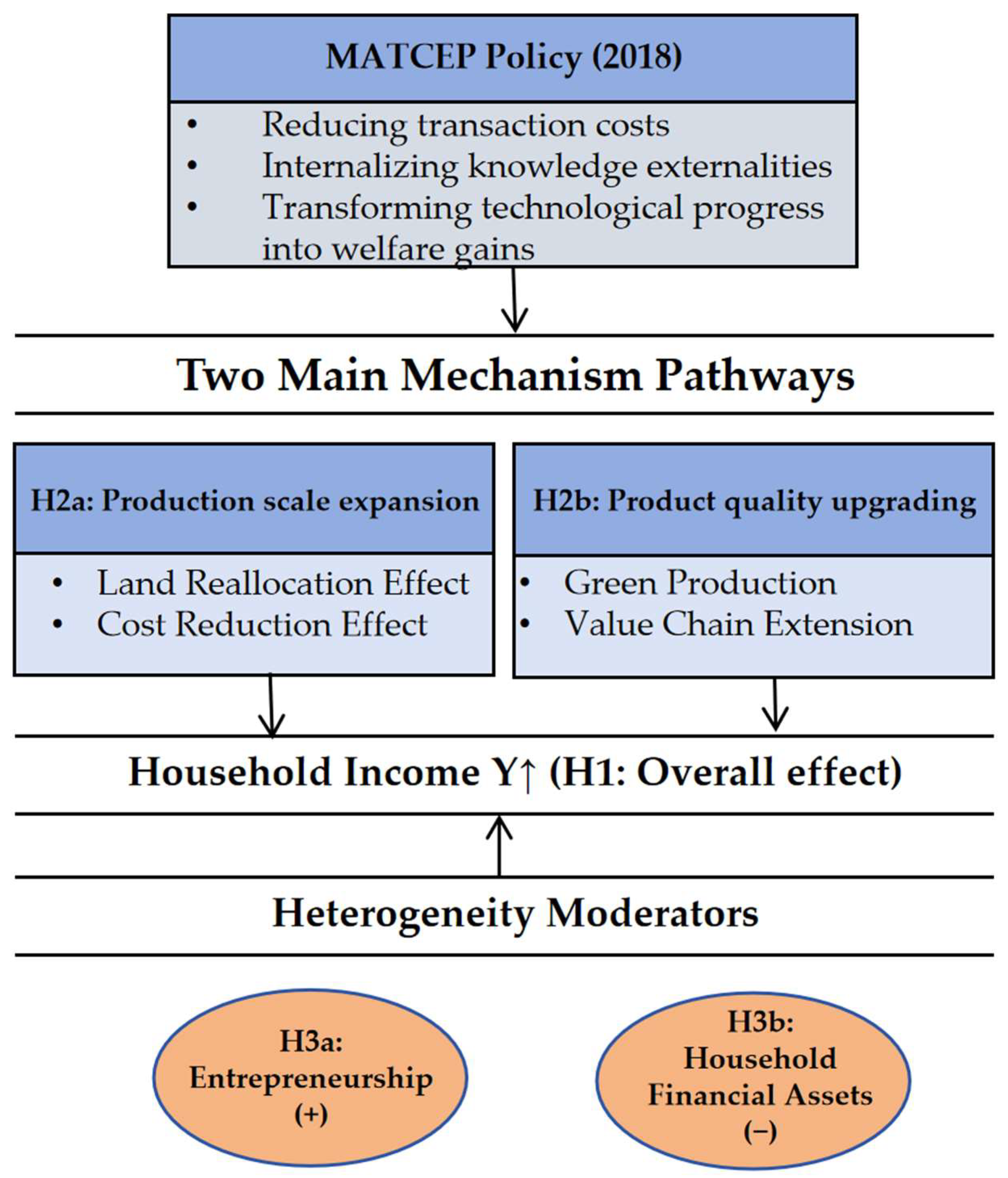
Figure 1. Mechanism Framework of the Collaborative Agricultural Technology Extension Program (MATCEP).
Economies 13 00331 g001
Figure 2. Event-study analysis of income effects under the Major Agricultural Technology Collaborative Extension Program (MATCEP). Estimated dynamic treatment coefficients for each year relative to policy implementation (s = 0); 95% confidence intervals displayed by vertical bars. All pre-treatment coefficients are statistically insignificant, confirming the parallel-trend assumption, while post-treatment years show significant positive effects on household income.
Economies 13 00331 g002
Figure 3. The standardized bias (Kernel Matching).
Economies 13 00331 g003
Figure 4. The propensity score distribution (Kernel Matching).
Economies 13 00331 g004
Figure 5. Kernel density plots of propensity scores before (left) and after (right) matching.
Economies 13 00331 g005
Figure 6. Placebo test of the virtual explanatory variable. The gray curve depicts the distribution of estimated coefficients obtained from 500 randomly assigned “false” policy treatments, while the black dots represent the corresponding p-values of each placebo regression. The horizontal dashed line indicates the 10% significance level (p = 0.1), and the vertical dashed line marks the true estimate from the baseline regression. As shown, most placebo estimates cluster closely around zero and lie above the 10% significance threshold, implying that few false policy effects are statistically significant. In contrast, the true estimate lies far to the right of the placebo distribution, suggesting that the observed policy effect is unlikely to arise from random chance and confirming the robustness of the empirical results.
Economies 13 00331 g006
Figure 7. Spatial Spillover Effects of the MATCEP on Household Income. Estimated income effects across concentric-distance intervals (0–2000 km) between provincial capitals; 95% confidence bands around each coefficient. Significant positive effects are observed within 1000 km, indicating geographically bounded spillovers through regional extension networks.
Economies 13 00331 g007
Table 1. Descriptive statistics.
VariableDefinition and UnitObs.MeanStd. Dev.MinMax
IncomePer capita household income (log, yuan)78231.26431.21790.002527.5000
PolicyAgricultural technology extension policy dummy: 1 = treated region-year, 0 = otherwise78230.05180.22160.00001.0000
ConsumptionPer capita total social consumption (log, yuan)782315.56780.966713.490718.7519
SchoolNumber of higher education institutions (log, units)78231.63950.89540.69314.4427
PhoneNumber of mobile phone users at year-end (log, 10,000 households)78235.93610.62164.00738.2848
LibraryTotal collection of public libraries (log, 1000 volumes/items)78237.32160.83675.771411.2765
EducationYears of schooling of household head78236.18054.19220.000016.0000
HealthHealth status of household head (1–5, higher = healthier)78232.87411.26191.00005.0000
RateLand transfer rate (%)78230.29700.09430.10090.8584
CostExpenditure on seeds, pesticides, and fertilizers (log, yuan)782313.28021.07226.908814.3060
OrganicNumber of organic food certifications (standardized)7823−0.00001.0000−0.91147.3061
ProcessNet increase in agricultural processing enterprises (log; absolute value taken if negative)78236.78481.6780−7.07079.6469
All log variables are calculated as ln(value + 1).
Table 2. Benchmark regression results.
VariablesModel 1Model 2Model 3
Policy0.2287 ***0.2474 ***0.2471 ***
(0.0765)(0.0773)(0.0772)
Consumption −0.2331 **−0.2303 **
(0.0984)(0.0985)
School −0.1974 **−0.1980 **
(0.0858)(0.0860)
Library 0.06310.0628
(0.0562)(0.0560)
Phone −0.0589−0.0614
(0.1434)(0.1439)
Education 0.0059
(0.0165)
Health 0.0111
(0.0140)
Cons1.2525 ***5.0920 ***4.9972 ***
(0.0040)(1.5635)(1.5617)
Individual FEsYESYESYES
Year FEsYESYESYES
Region FEsYESYESYES
R 2 0.57180.57340.5735
N782378237823
In this table, **, and *** denote statistical significance at the 5%, and 1% levels, respectively. Robust standard errors clustered at the household level are reported in parentheses.
Table 3. Pre-trend Test Results.
TestStatistic
Pre-treatment joint testF = 0.48
p = 0.6194
Post-treatment joint testF = 6.15
p = 0.0004
Covariates × year interaction joint pre-test (excluding post-treatment periods)F = 1.43
p = 0.2388
Table 4. Results of robustness test for omitted variables (Ratio Method).
Restricted Specification (A)Full Specification (B)Ratio
Only fixed effects
(individual + year + region)
All controls + fixed effects (individual + year + region)13.4183
Regional controls + fixed effects
(individual + year + region)
All controls + fixed effects (individual + year + region)953.0489
Household controls + fixed effects
(individual + year + region)
All controls + fixed effects (individual + year + region)13.1167
Table 5. Balance Test Results (Kernel Matching).
VariablesMatching StatusTreated MeanControl Mean% Biast-Valuep-Value
ConsumptionBefore matching15.70115.55315.34.110.000
After matching15.70115.682.20.440.659
SchoolBefore matching1.69591.63317.01.880.060
After matching1.69591.6993−0.4−0.070.942
LibraryBefore matching7.50507.300622.16.570.000
After matching7.50507.43737.31.410.158
PhoneBefore matching5.89735.9405−6.6−1.870.062
After matching5.89735.9086−1.7−0.340.733
EducationBefore matching5.93526.2085−6.5−1.750.080
After matching5.93525.9893−1.3−0.260.796
HealthBefore matching2.75972.8872−10.1−2.710.007
After matching2.75972.7783−1.5−0.300.766
Table 6. The PSM-DID Regression Results.
VariablesModel 1Model 2Model 3Model 4
Policy0.2530 ***0.2515 ***0.2291 *0.2530 ***
(0.0779)(0.0780)(0.1280)(0.0779)
Consumption−0.2325 **−0.2403 **−0.2570−0.2325 **
(0.1043)(0.1051)(0.1733)(0.1043)
School−0.2045 **−0.2057 **−0.1832−0.2045 **
(0.0876)(0.0877)(0.2129)(0.0876)
Library0.07430.07460.12910.0743
(0.0614)(0.0636)(0.1188)(0.0614)
Phone−0.1720−0.1731−0.2131−0.1720
(0.1749)(0.1755)(0.5855)(0.1749)
Education0.00720.0065−0.01550.0072
(0.0166)(0.0166)(0.0273)(0.0166)
Health0.01640.01610.01060.0164
(0.0142)(0.0143)(0.0298)(0.0142)
Cons5.5912 ***5.7245 ***6.0854 *5.5912 ***
(1.6837)(1.6865)(3.1859)(1.6837)
Individual FEsYESYESYESYES
Year FEsYESYESYESYES
Region FEsYESYESYESYES
R 2 0.57740.57750.74900.5774
N7703768524497703
In this table, *, **, and *** denote statistical significance at the 10%, 5%, and 1% levels, respectively. Robust standard errors clustered at the household level are reported in parentheses.
Table 7. Results of the placebo test with the policy implementation year moved up two years.
CoefficientStd. Errorz-Valuep-Value95% Confidence Interval
0.05830.11610.500.615[−0.1693, 0.2860]
Table 8. Results of robustness test.
VariablesModel 1Model 2Model 3Model 4Model 5
Alternative
Outcome
Variable
Winsorization at 1%Winsorization at 5%Excluding
Municipalities
Excluding
Concurrent
Policy Interventions
Policy0.0930 **0.2385 ***0.2471 ***0.2457 ***0.2316 ***
(0.0443)(0.0714)(0.0772)(0.0773)(0.0776)
Consumption−0.1100 **−0.2772 ***−0.2303 **−0.2264 **−0.2371 **
(0.0500)(0.0693)(0.0985)(0.0995)(0.0984)
School−0.1756 ***−0.1522 **−0.1980 **−0.1986 **−0.2239 **
(0.0541)(0.0712)(0.0860)(0.0861)(0.0877)
Library0.03230.05350.06280.06360.0523
(0.0357)(0.0513)(0.0560)(0.0561)(0.0562)
Phone−0.1982 **−0.0723−0.0614−0.0581−0.0733
(0.0845)(0.1259)(0.1439)(0.1444)(0.1438)
Education0.00680.00550.00590.00580.0068
(0.0102)(0.0140)(0.0165)(0.0165)(0.0165)
Health−0.00600.00730.01110.00960.0101
(0.0105)(0.0118)(0.0140)(0.0142)(0.0140)
Digi 0.1688
(0.1226)
Cons12.1219 ***5.7738 ***4.9972 ***4.9087 ***5.2862 ***
(0.8427)(1.2131)(1.5617)(1.5778)(1.5563)
Individual FEsYESYESYESYESYES
Year FEsYESYESYESYESYES
Region FEsYESYESYESYESYES
R 2 0.63420.60960.57350.57250.5737
N78237823782377507823
In this table, **, and *** denote statistical significance at the 5%, and 1% levels, respectively. Robust standard errors clustered at the household level are reported in parentheses.
Table 9. Mechanism Analysis Results.
VariablesModel 1Model 2Model 3Model 4
LandCostOrganicProcess
Policy0.0381 ***−0.1179 ***0.5862 ***1.4479 ***
(0.0046)(0.0204)(0.0581)(0.2055)
Consumption−0.0700 ***0.0916 ***0.7031 ***0.3417 ***
(0.0042)(0.0161)(0.0755)(0.1058)
School0.0054−0.0375 ***0.0290−0.0403
(0.0046)(0.0122)(0.0591)(0.0613)
Library0.0137 ***0.1169 ***0.1547 **−0.0280
(0.0026)(0.0149)(0.0602)(0.0377)
Phone0.0491 ***−0.0919 ***−0.00960.1468
(0.0086)(0.0228)(0.0779)(0.1080)
Education−0.0021 ***0.0109 ***0.00060.0122
(0.0007)(0.0037)(0.0100)(0.0161)
Health0.0012 *0.0005−0.0068−0.0015
(0.0006)(0.0028)(0.0090)(0.0148)
Cons0.9933 ***11.5431 ***−12.0833 ***0.7188
(0.0820)(0.2698)(1.4220)(1.8497)
Individual FEsYESYESYESYES
Year FEsYESYESYESYES
Region FEsYESYESYESYES
R 2 0.87770.97820.77610.7310
N7823782378237823
In this table, *, **, and *** denote statistical significance at the 10%, 5%, and 1% levels, respectively. Robust standard errors clustered at the household level are reported in parentheses.
Table 10. Heterogeneity Analysis Results.
VariablesModel 1Model 2
Policy0.1992 ***0.3835 ***
(0.0764)(0.0960)
Entrepreneurship0.0175-
(0.1187)
Policy × Entrepreneurship0.6895 **-
(0.3511)
Financial assets-0.0163 ***
(0.0036)
Policy × Financial assets-−0.0260 **
(0.0119)
Consumption−0.2374 **−0.2334 **
(0.0981)(0.0981)
School−0.1982 **−0.1720 **
(0.0858)(0.0839)
Library0.06410.0463
(0.0560)(0.0558)
Phone−0.0567−0.0408
(0.1437)(0.1431)
Education0.00600.0056
(0.0165)(0.0164)
Health0.01120.0116
(0.0140)(0.0140)
Cons5.0692 ***4.9212 ***
(1.5593)(1.5576)
Individual FEsYESYES
Year FEsYESYES
Region FEsYESYES
R 2 0.57410.7369
N78232536
In this table, **, and *** denote statistical significance at the 5%, and 1% levels, respectively. Robust standard errors clustered at the household level are reported in parentheses.
Table 11. Global perspective on agricultural extension comparison.
DimensionUnited States (Education–Research–Extension Triad)Japan
(Government–Cooperative Dual-Track)
Thailand
(High-Density, Donor-Supported Network)
Brazil
(Pluralistic Family-Farming Model)
Ethiopia
(Public Mass-Extension System)
China (MATCEP, Collaborative Extension)
Governance & OwnershipFederally legislated Smith–Lever Act (1914); shared governance among USDA, land-grant universities, and county governments; public ownership, decentralized execution.Dual-track system: government line agencies (MAFF) + legally autonomous agricultural cooperatives under the Agricultural Cooperative Act (1990); strong vertical accountability.Centralized Ministry of Agriculture with 5-tier hierarchy (national → district → sub-district); coordination through provincial offices; World Bank oversight.Multi-actor governance under PNATER (2004/2010); Ministry of Agrarian Development leads, NGOs and cooperatives co-implement; participatory councils ensure inclusiveness.Strongly centralized under the Ministry of Agriculture; extension agents are public employees; administrative accountability dominates.State-led but collaborative: MARA designs policy, provinces implement; partnerships among universities, cooperatives, and firms institutionalized under MATCEP (2018).
Financing MechanismMixed funding: 20–25% federal/50% state/25% county; stable, legally mandated budgets; performance-based grants for innovation.50–50% cost sharing between central and prefectural governments; cooperatives finance member-specific services through fees and retained earnings.~70% financed by World Bank loans + 30% domestic co-funding; heavy external-aid dependence; declining sustainability after donor withdrawal.Federal–state cost sharing + competitive contracts; NGOs obtain project-based funds; annual budget volatility ±30%.>90% public funding from national treasury; local cost-sharing minimal; CAADP target (10% of public expenditure) achieved.Public funding from MARA + provincial matching; enterprises and cooperatives contribute in demonstration projects; gradually expanding cost-sharing mechanism.
Delivery & Accountability2900 county offices; staff often PhD-level specialists; 4-H and Master Farmer programs; performance audited by USDA/NIFA outcome metrics.Extension officers (technical + diffusion agents) provide onsite training; cooperatives accountable to elected boards; evaluation via MAFF KPIs.One extension worker per ~1000 farmers; multi-service package (technology, finance, marketing); annual audits by World Bank project units.Participatory delivery through family-farm organizations and NGOs; user-feedback integrated via rural councils; accountability horizontal rather than hierarchical.47,000 Development Agents across 15,000 Farmers Training Centers; standardized “technology package” dissemination; administrative reporting to district offices.Provincial technology taskforces manage demonstration bases; evaluation combines output indicators (income growth, adoption rate) and peer review by research institutes.
Knowledge & Innovation LinkagesStrong university–research–extension continuum; experiment stations feed innovations directly into extension curricula; digital agriculture integration.Applied research within prefectural experiment stations; MAFF funds national R&D on rice, horticulture; knowledge flows through cooperative networks.Weak research interface; technology supplied via donor-backed projects and international consultants; limited local R&D absorption.Multi-directional learning: universities + EMATER + farmer field schools; emphasizes agro-ecology and social innovation; bottom-up feedback mechanisms.Close linkage between research centers and DA/FTC network; limited feedback to national R&D; ongoing “Digital Green” ICT pilot improves flow.Integrates universities, academies, and enterprises; collaborative innovation platforms align research agendas with production demand; two-way feedback institutionalized.
Sources: United States data are compiled from the U.S. Department of Agriculture (USDA) official website and the Smith–Lever Act of 1914. Japan’s information derives from the Ministry of Agriculture, Forestry and Fisheries (MAFF) reports and the Agricultural Cooperative Act of 1947. Thailand’s system description and statistics are drawn from World Bank project documents and the Ministry of Agriculture and Cooperatives (MOAC) datasets. Brazil’s data are based on the National Policy for Technical Assistance and Rural Extension (PNATER) and the EMATER official publications. Ethiopia’s information references the Comprehensive Africa Agriculture Development Programme (CAADP) progress reports and the Federal Ministry of Agriculture white papers. China’s data originate from the Ministry of Agriculture and Rural Affairs (MARA) announcements and the Major Agricultural Technology Collaborative Extension Program (MATCEP) Implementation Plan.
Disclaimer/Publisher’s Note: The statements, opinions and data contained in all publications are solely those of the individual author(s) and contributor(s) and not of MDPI and/or the editor(s). MDPI and/or the editor(s) disclaim responsibility for any injury to people or property resulting from any ideas, methods, instructions or products referred to in the content.