Abstract
The purpose of this work is twofold: first, it aims to derive an exact analytical form of the Pareto index based on the already developed model of the economy as a scale-free network comprising a given amount of either wealth or income (total number of links, each link representing a non-zero amount or quantum of income or wealth) distributed among its variable number of actors (nodes), all of whom have equal access to the system), and second, it aims to employ the derived analytical form of the Pareto index to determine the degree to which the observed inequality in wealth and in income as measured by the respective empirical values of the Pareto index is inherent in the economic system rather than the result of externally imposed factors invariably reflecting a lack of equal access. The derived analytical form of the Pareto index for wealth or for income is described by an exponential function whose exponent is the inverse of the average number of wealth or of income per actor (one-half of the average number of links per node) in the economic model. This exponent features prominently in the scale-free model of the economy and has a numerical value of 0.69 when the Pareto index attains a numerical value of 2, which signifies the optimal, albeit still unequal, distribution of wealth or of income in the economy under the condition of equal access. Because of the correspondence of the scale-free model of the economy to a physical system comprising quantum particles such as photons in thermodynamic equilibrium or state of maximum entropy in accordance with the laws of statistical mechanics, the inverse of the exponent is proportional to the temperature of the economic system, and a new parameter introduced to describe in a comprehensible manner the deviation in the economic system from its optimal distribution of wealth or income. A comparison of the empirical wealth and income Pareto indexes based on economic data for the four largest economies in the word, i.e., USA, China, Germany, and Japan, which account for over 50% of the global GDP, versus the corresponding optimal values per the scale-free model of the economy reveals interesting trends that can be explained away by the prevailing degrees of equal access, as manifested by inadequate education, health care, and housing, as well as the existence of rules and institutions favoring certain actors over others, particularly with regard to the accumulation of wealth. It has also been determined that the newly introduced parameters in the scale-free model of the economy of temperature as well as the quanta of wealth and of income should be expressed in power purchase exchange rates for meaningful comparisons among national economies over time.
1. Introduction
A scale-free network to represent an economic system has recently been developed by us, whereby the members or actors of the system are represented as nodes and the wealth or income is represented by the corresponding total number of links associated with each node (Ingersoll, 2024). The connection between a scale-free network and an eco-nomic system is based on the fact that the former is described analytically by a power law, while the distribution of wealth and of income is known empirically to follow a Pareto law, which is a power law (Barabási, 2014; Pareto, 1925). Moreover, researchers have demonstrated that a scale-free network is analogous to a thermodynamic system comprising a very large number of quantum particles such as photons representing the links occupying different energy states, each of which refers to an actor (Bianconi & Barabási, 2001). The significance of the analogy of a scale-free network to a physical system comprising quantum rather than classical particles will become apparent shortly. Thus, our model of the economy as a scale-free network is akin to a thermodynamic system comprising quantum particles occupying different energy states. The energy states reflect the nodes in the scale-free model and, thus, the actors comprising the economic systems. The quantum particles correspond to the number of links associated with each node, a link describing the quantum unit of wealth or of income, which is finite, i.e., non-zero. The total number of links per node represents then the wealth or the income associated with the corresponding actor in the economic system. A thermodynamic system attains a state of equilibrium determined uniquely by the available total energy at a particular moment in time by reaching a state of maximum entropy according to the laws of statistical thermodynamics (Schrödinger, 1944/1989). Moreover, the total energy of a quantum system is only known within the quantum of action (energy × time). Consequently, an economic system as a scale-free network attains a state of equilibrium based on the available total wealth or total income at any particular moment in time. The physical quantum of action (Planck’s constant) is translated into or is analogous to the already-mentioned quantum of wealth and of income in the economic system, two critical parameters to be addressed in detail later in this article. Two important conditions associated with physical systems comprising quantum particles such as photons are that there are an infinite number of possible energy levels and the particles are indistinguishable. These conditions translate into the economic system via the scale-free network model by reflecting a variable, i.e., not-fixed, number of actors (nodes), with each actor having equal access, i.e., probability, to the available wealth or income (number of links). It should be noted that the variable number of actors does not preclude actors with zero links (wealth or income) from being part of the system. Because of the variable number of actors and the equal probability of each actor having access to wealth or income, an actor (node) with zero wealth or income (links) may attain a finite number, while another actor with a finite amount of wealth or income may lose it all (zero links). The key thing to remember is that a link is proportional to the quantum of wealth or of income. The scale-free model of the economy, as described, leads then quite naturally into the derivation of the Pareto distribution of the wealth or of the income among the actors and provides an analytical expression of the Pareto index as a function of certain parameters of the economic system (Ingersoll, 2024). Moreover, this model suggests that there is a particular value for the Pareto index that leads to the most optimal distribution of wealth and of income among the members of the economic system. Lastly, the model of the economy as a scale-free system helps shed light, and perhaps even answers conclusively, in our view, a very important question that has been debated by economists for a long time, namely, equal access vs. equal outcome (Deaton, 2013). Equal access would guarantee, in the absence of external biases, the most optimal, albeit still unequal, outcome. Moreover, equal outcome would not only be impossible to attain but would also result in inefficient use of finite resources and ultimately could exacerbate inequality by dealing with the symptoms rather than addressing the causes of excessive inequality.
The distribution of wealth or of income in the economic system as a scale-free net-work with all actors having equal access or opportunity in it is tantamount to the system becoming hierarchical to confer maximum stability, i.e., maximum entropy, to the system. Thus, certain actors end up with more wealth or income than most: equal opportunity leads to unequal outcome. An optimal value of the Pareto index at 2 represents the most efficient allocation of the available wealth or income among all the members of the eco-nomic system. However, the occurring wealth and income in actual economic systems clearly suggests that both income and, particularly, wealth are not distributed in accordance with the optimal Pareto index value (Ingersoll, 2024). Obviously, there are exogenous factors at work that exist within any economic system imposed either based on the faulty assumption of equal opportunity or deliberately to favor certain actors or a combination of both (Susskind, 2024). Moreover, there is abundant evidence of a lack of equal opportunity (Piketty, 2024; Susskind, 2024). The application of taxation and payment transfers to correct the perceived inequality of the outcome is inefficient because it deals with the symptoms rather than the root cause of the problem, i.e., a lack of equal opportunity. Moreover, the promotion of regulations and institutions favoring certain actors exacerbates further the lack of equal opportunity. We may also mention that how the concept of Parero optimality of the standard economic theory relates, if at all, to the Pareto optimal index of two per the scale-free model of the economy would require research effort beyond the scope of this work.
The application of fundamental principles and concepts from physics, particularly statistical mechanics and thermodynamics, to economics, of which the scale-free model of the economy is a very recent one, has had a rather long history, starting at the end of the 19th century (Pareto, 1925). However, the emphasis has been all along on finance rather than economic theory, and whenever economic theory is addressed, random networks are invariably employed (Mantegna & Stanley, 2000; Mandelbrot & Hudson, 2006; Greenberg & Gao, 2024). A critical distinction between the traditionally favored random networks in economic theory vs. scale-free networks advanced by us is that the former display Gaussian or bell-curve distributions and the latter display Pareto or power law distributions (Barabási, 2014). The objective of this work as a sequel to the already published model of the economic system as a scale-free network is twofold: (a) to derive an exact analytical expression of the Pareto index as a function of the two key parameters that describe the scale-free model of the economy, namely, the average wealth or income per actor and the quantum of wealth or income; and (b) to obtain practical new parameters to measure the inequality in opportunity such that corrective actions can be implemented to deal with the underlying causes.
2. Summary of the Model of the Economy as a Scale-Free Network
The development of the model of the economy as a scale-free network is founded on the empirical observation that a power law, i.e., the Pareto law, describes the distribution of wealth and of income (Pareto, 1925). Moreover, there has been a recent realization in physics that power laws describe the collective behavior of groups of identical or indistinguishable, i.e., quantum, particles, leading to a phase-change state (Bianconi & Barabási, 2001). In other words, the collective behavior of such particles can be modeled as a scale-free network, where the possible energy levels of the system of particles represent the nodes, while the number of particles occupying a particular energy level or node represents the links associated with that node (Barabási, 2014). In essence then, the principles of statistical mechanics and thermodynamics are applicable to the description of the model of the economy as a scale-free network. Table 1 provides the mapping of the economic system to a scale-free network and to a physical system comprising quantum particles (Ingersoll, 2024). The application of statistical mechanics principles obtains the state of equilibrium when the entropy of the system reaches a maximum value under the constraint that the physical system is at a given fixed temperature or total available energy. The latter quantity corresponds to the total wealth or income of the economic system.

Table 1.
Schematic of the mapping of the economic system into a scale-free complex network and its modeling as a Planck photon gas physical system.
The economic model as a scale-free network consists of N actors with a total wealth U to be distributed among these actors, if all these actors have equal opportunity to a portion of the total wealth. This access to equal opportunity is tantamount to the treatment of the quantum particles in the statistical mechanics model as being indistinguishable.1 Moreover, there is a minimum amount of wealth designated by h, the so-called quantum of wealth and a counterpart quantum of income. This is the minimum amount of wealth or income an actor may acquire as part of the economic system. It should be noted that the scale-free model of the economic system does not exclude actors with zero wealth or income, given that the number of actors is variable such that actors can enter or leave the system as they acquire or lose wealth or income depending on the parameters of the economic system itself. Obviously, the numerical value of h for wealth would be different than that for income. In the free-scale network model of the economy, actors are represented by nodes, and the wealth or income of each actor would be equal to one-half the number of links associated with that actor times the quantum of wealth or income, respectively. This is due to the mathematical description of the complex network according to the so-called graph theory (Trudeau, 1993). A graph comprises vertices (nodes) and edges (links). The number of edges (links) attached to each vertex (node) is designated as the degree of that vertex. An edge (link) connects two vertices (nodes). Thus, each link is multiplied by twice the quantum of wealth or income (one quantum per actor), and this represents the wealth or income shared by the respective two actors. Then, each actor owns one-half of that wealth or income in a system where all actors have equal access to it. Thus, we obtain for the scale-free network model of the economy consisting of N nodes and with a total number of links K the equation:
Thus, K/N = represents the average number of links per node and is equal to one-half of the average wealth or income per actor as a multiple of the quantum of wealth or income h as already indicated. The quantity (1/βh) is analogous to the average energy per oscillator in the thermodynamic analogy of the scale-free network as a system of quantum particles in a physical system kept at a temperature T, whereby 1/β can be then viewed as the “temperature” of the economic system. We note then that for the economic system:
If β is high, its temperature is low, and if β is low, its temperature is high.
We will address later in this article the implications of the temperature concept as it pertains to an economic system.
The probability density function ϕ(x) and the cumulative distribution function Φ(x) of the economic system with a varying number of actors N as a function of the normalized random variable x = X/h, where X is the wealth, is then (Ingersoll, 2024):2
Φ(x) = 1 − x−δ x ≥ 1
δ ≥ 1 and δ = 2 at the maximum of ϕ(x) for any x
Eδ(nβh) = ∫ (exp (−nβhx)/xδ) dx for (βh) > 0, δ = 1, 2, 3, …, n = 1, 2, 3, …
The function Eδ(nβh) is the exponential integral function, also known as the Schlömilch function, and is described by Equation (8) (Abramowitz & Stegun, 1972) (Zwillinger, 2012). The parameter δ is identified with the Pareto index per Equations (3) and (4), and it has a minimum value of 1 and an optimal value of 2 per Equation (7). The latter is dictated by the fact that in the original derivation δ is an integer per the definition of the exponential integral functions and the nature of the ϕ(x) function per Equation (3), which is a monotonically decreasing function with an increasing argument x. Equation (5) provides an upper bound of the value of δ or the Pareto index. The objective of this work is to develop a closed-form analytical expression for the Pareto index to replace the originally derived upper bound infinite series expression per Equation (5) while relaxing the constraint on δ to be any real number, rather than an integer greater than one. The optimal value of δ = 2 represents the maximum value of the probability density function ϕ(x) at any x greater or equal to one. The upper bound of the Pareto Index δ is given analytically by Equation (5) as a function of the parameter (βh), the inverse of which reflects the average number of links per node per Equation (1) in the scale-free network representing the economic system. Employing Equation (5), we obtain the approximate value of (βh) of about 0.67, as shown in Table 2 per the optimal value of δ = 2 per Equation (7).3
Table 2.
Numerical calculation of the value of the parameter (βh) for which the Pareto index attains the optimal value of δ = 2 values based on the ratio of the sums of the exponential integral functions E1(βh) and E2(βh) for up to fourteen terms (n = 14).
The approximate value of (βh) of about 0.67 indicates that the optimal distribution of wealth or of income in the economic system described by a scale-free network occurs when the average number of links per node Ko equals about 1.49 (1/0.67). Any deviation from Ko will result in a suboptimal distribution of a fixed amount of wealth or income among the N actors comprising the economic system. Since the number of actors N is not fixed, anytime a change in N would occur, there would be a temporary change in the value of Ko until equilibrium occurs, i.e., the economic system reaches maximum entropy again, and Ko obtains the new optimal value. The assumption for the Ko value to be obtained is that all actors in the system have equal access to wealth or income. If this is not true, then the value of K will remain higher or lower than Ko. We will address later in this article the issue of sub-optimal values of K that are different from Ko. We may also note that the so-called quantum of wealth or income h is different to the unit of currency in the economy that we assumed in the original derivation of the Pareto Law from first principles (Ingersoll, 2024). We now conclude that h represents an average amount of wealth or of income per actor that is specific to a particular economic system. Thus, we would have an hw for wealth and an hi for income in any given economy. However, the Ko value is a constant, thereby indicating that the value of the parameter β will be also different for wealth and for income in the economic system.
Given that Equation (5) provides an upper bound of the value of the Pareto index as a function of the average number of links (average wealth or income) per node (actor) in the economic system as a scale-free network, we will derive an exact and easier-to-use formulation.
3. Previous Work in Scale-Free Networks Applicable to the Economic Model
The impetus for this work is based on two key elements as follows (Ingersoll, 2024): (a) the empirical observation at the beginning of the 20th century that wealth distribution is described by a power law, which is also known as the Pareto law or principle in economic theory (Pareto Principle, 2024); and (b) the realization in the early 21st century that power laws can be described or modeled by scale-free networks as opposed to random networks (Barabási, 2014). A rough enunciation of the Pareto law states that 20% of the population owns 80% of the wealth and is abbreviated as the 80–20 law (Newman, 2006). Income distribution was also found to obey the same law. The “80–20% Pareto Principle” applies to several other situations such as the world-wide web, where 80% of links point to only 15% of webpages, scientific articles, where 80% of citations go to only 38% of scientists, movie celebrities, where 80% of links in Hollywood are connected to 30% of the actors, and numerous more mundane occurrences (Barabási, 2014). We may also mention that, in contrast to scale-free networks, multiple aspects of nature are described by random networks, such as the height or weight of living organisms or the grade distribution of students in school. Random networks are described by the well-known bell curve, i.e., a peak value and fast decaying tails. As the name suggests, a quantity x described by a power law would have the following generic functional dependency:
which is essentially similar to the probability density function per Equation (3) of the distribution of wealth or income in an economic system. The parameter δ, known as the Pareto index, is a number characteristic of the particular system described by Equation (9). Studies have concluded that the value of the Pareto index can vary, as shown in Table 3 for several relevant systems (Barabási & Albert, 1999; Adamic & Huberman, 2000; Redner, 1998). To this we have added the global economy as represented by its Pareto index (Ingersoll, 2024).4 It should be noted that in the already-quoted earlier studies on scale-free networks, the random variable x per Equation (9) represents the number of links k per node (actor) in the system, which of course is proportional to the wealth or income in the economic model per Equation (1), as already described. We may also mention that the Greek letter γ has been used in earlier studies to describe the Pareto index versus the Greek letter δ employed by us in our model of the economy as a scale-free network. Lastly, the average connectivity per node in the scale-free networks included in Table 3 range from a high of 28.78 for movie actor collaboration to 5.46 for the world-wide web and to 2.67 for the power grid (Barabási & Albert, 1999). For the model of the economy as a scale-free network, the optimal value of the average connectivity should be about 1.49 (1/0.67), as already discussed. However, the current average connectivity for wealth and for income will be obtained via a suitable model to be developed in this work.
Table 3.
Pareto index for several systems governed by a power law and modeled as scale-free networks.
Historically, networks of complex topology have traditionally been described with the random graph theory developed by Erdos and Renyi during the second half of the 20th century (Barabási, 2014; Trudeau, 1993).5 However, the structure of the developing world-wide web (WWW) coupled with advances in the understanding of condensed-matter physics toward the end of the 20th and the beginning of the 21st centuries has led to the realization that large-scale networks display self-organization properties that are consistent with a power law description per Equation (9) and, hence, a scale-free state. This feature of large scale-free networks is contrary to the evolution of a random network. That is to say, random networks fail to incorporate the growth of nodes and the preferential attachment of nodes via links to other nodes in a scale-invariant form. Scale-free networks consist of most nodes having a few links coexisting with a few big hubs, i.e., nodes with an anomalously high number of links, in a hierarchical fashion such that the relatively small number of big hubs are connected to the relatively larger number of smaller hubs down to the nodes with a few links to ensure that all the nodes are fully connected, and the network is kept functioning. A random network has a characteristic scale in its node connectivity described by a peak node with the maximum number of links and a distribution of nodes with fewer links following a bell curve. It appeared that in a scale-free network, the nodes and links would arrange themselves in an orderly fashion to obtain the scale-free hierarchical status. But how would that happen? This is where statistical mechanics or thermodynamics came in gradually during the last few decades of the 20th century to explain the so-called condensation or phase transition of quantum particles into a state of order from disorder, which is attained by the forces of self-organization and is described by power laws (Barabási, 2014).
Based on these scientific developments, an analytical model was developed at the turn of the 21st century describing the evolution of a scale-free network over time and dis-playing the resulting power law characteristic feature (Barabási & Albert, 1999; Bianconi & Barabási, 2000, 2001). In addition, while this model clearly demonstrated the power law feature of the scale-free network, it suffered from two fundamental limitations as follows: (a) preferential attachment, such that well-connected nodes are more likely to gain new links; and (b) continuous growth over time, such that nodes are constantly added to the network. In particular, the constant growth aspect is unrealistic in most real-world scale-free networks. This eternal growth limitation of the earlier model has been remedied very recently by the development of an emergent scale-free network model, where the scale-free structure can arise without requiring continuous growth (Lynn et al., 2024). In this model, a combination of node death along with preferential attachment and random attachment of the freed-up links leads to a steady-state but dynamic model of a scale-free network. The scale-free index γ calculated by this model is given by a simple equation of the following form:6
with p = 1 for 100% preferential to p = 0 for 100% random attachments. The range of values for the index γ from two to infinite.
γ = 1 + 1/p … where 0 ≤ p ≤ 1, p is the probability of attachment of a link to a node
This steady-state model represents a significant improvement over the original time-dependent model of over twenty years ago in several aspects for a realistic description of a scale-free network as follows: (a) the model does not depend on constant node growth, which is unrealistic in most real-world scale-free networks; (b) it allows for the death or removal of nodes in the network as well the creation of new nodes, such that the number can be reduced or increased and not remain constant; (c) it provides a scale-free index with a wide range of values, which is typically encountered in real-world situations;7 and (d) it has an index value of two when all nodes display a preferential attachment rather than a random one. We may also note that our model of the economy as a scale-free network is in general consistent with (i) the steady-state dynamic model, including the steady state nature of it, (ii) the variability in the numbers of actors in the system, and (iii) the ability to predict a wide range for the scale-free index or Pareto index with an optimal value of two. We may also note that the application of statistical mechanics principles in the development of the model of the economy as a scale-free network naturally avoids the introduction of the time evolution that has been problematic with the earlier scale-free network models, as already discussed. Statistical mechanics employs the concept of substituting the time evolution of any given system with a large ensemble of such systems to obtain the most probable representation of the system under consideration (Schrödinger, 1944/1989).
4. The Analytical Formulation of the Pareto Index in the Scale-Free Model of the Economy
A simple analytical model for the calculation of the Pareto index will be developed next to complement the already-developed scale-free model of the economy (Ingersoll, 2024). We note that in the original derivation of the scale-free network model of the economy, as summarized in Section 2, the parameter δ, identified as the Pareto index, assumes only integer values greater than or equal to one. This was the result of our assumption that the exponential integral Eδ(βh) function is defined for an integer index to simplify the calculations (Abramowitz & Stegun, 1972). Consequently, the next higher value of δ greater than one is two, as stated in Equation (7). The probability distribution function ϕ(x) per Equation (3) attains at δ =2 a higher value as x increases, i.e., it has a fatter tail or decays slower, than at any value higher than δ = 2 (Pareto Distribution, 2025; Ingersoll, 2024). Hence, the Pareto index of 2 signifies what we call the optimal value for wealth and income distribution. We know that the Pareto index or shape factor can take any positive value greater than one, such that the expected value of the stochastic variable x described by the Pareto distribution is finite (Pareto Distribution, 2025). Moreover, the Pareto index or shape factor of a stochastic variable x described by a Pareto distribution must be higher than two for the variance of the stochastic variable to remain finite (Pareto Distribution, 2025). We also note that the empirically calculated values of the power law index of various scale-free networks per Table 3 are higher than two, with that of the world-wide web approaching two. However, the power law index of the global economy is less than two. We also note that the power law index of scale-free networks as calculated independently by others attains the minimum value of two per Equation (10) as well.
The intent here is then to reconcile all these findings to derive a readily useable formula that is both exact and consistent with the scale-free network model of the economy that has, in turn, as its foundation the employment of statistical mechanics or thermodynamics. In this development process, we will also determine how we can account for the observed difference between the distribution of wealth and income in the real world, as manifested by different Gini coefficients for wealth and for income and, consequently, Pareto indexes. We may note that a distinction between wealth and income is manifested in the analytical model of the economy as a scale-free complex network with respect to the differentiation of so-called quantum of wealth and quantum of income already discussed to some degree in Section 2.
Based on the results per Equations (5) and (7) of the Pareto index as well as the determination of the value of the parameter (βh) when the Pareto index has the optimal value δ = 2, we require heuristically, but also consistently with Equation (5), that the functional form of δ would be as follows:
δ = 1 + f(βh) … where f(βh) is a monotonically increasing function of (βh)
We may note that the numerical value of (βh) per Equation (13) is based on the upper bound of δ per Equation (5), and an exact value of it will be obtained shortly. The functional format of δ per Equation (11) has been selected such that minimum value of δ would be at least one at a certain value of the parameter (βh) to be determined. This also implies that the value of the function f(βh) would also tend to zero at that value of the parameter (βh). It should be noted that Equations (11)–(13) for the Pareto index δ have a similar format as Equation (10), although the parameter p in that equation is different from the function f(βh) in Equation (11). However, we may also note that in Equation (10), the parameter p may be interpreted to mean the degree to which nodes (actors) in the system to which γ would apply are hierarchically connected. Thus, p = 1 signifies an absolutely perfect hierarchical structure, i.e., all nodes have equal access, and a p < 1 indicates a breakdown of the hierarchical structure with external biases introduced to make the system deviate from its optimal configuration. As we have already indicated, a scale-free network where all nodes have equal probability to have a link attached to them attains its most stable configuration (maximum entropy) and displays the optimal distribution of links among its nodes. In that instance, the Pareto index, whether it is given by Equation (10) or Equation (11), attains a numerical value of 2, which signifies, in our view and as already explained, the optimal configuration of the node–link distribution of the scale-free network for the hierarchically most stable system. We may also note that a distinct advantage of the formulation of the Pareto index per Equations (11)–(13) is that δ can also attain values less than 2, which are observed in the system of the economy as the data in Table 3 clearly indicate. We would also like to reiterate that a system such as the global economy that is described empirically by the Pareto distribution and has a power law index or Pareto index less than two has consequently an infinite, i.e., non-finite, variance. Such a system has an unpredictable level of dispersion and is prone to producing outcomes that are vastly different from the average. That is to say, the prevailing economic system globally has diminished hierarchical stability and is characterized by the occurrence of more extreme gains or losses that would otherwise be expected. We have already alluded to and will be discussing in greater detail the reasons that have been responsible for the large deviation in the economy from its optimal state.
In the earliest model of a scale-free network the concept of fitness was introduced to describe the ability of a node to attract links preferentially over time (Bianconi & Barabási, 2000). This feature would then lead to a power law as the network evolved in time. In our model of the economy as a scale-free network there was no need to consider the fitness concept or time evolution, as a different approach was followed based on statistical mechanics that replaces time with ensemble averages and where all actors (nodes) have equal access or probability to wealth (links) (Ingersoll, 2024). In another recently published model of an emergent scale-free network that represents a steady-state, i.e., it is not an explicitly time-dependent system, the freed-up links were assigned a probability p to be preferentially attached to other nodes, while (1 − p) would be the probability of a random attachment, and the scale-free index per Equation (10) would be obtained (Lynn et al., 2024). In order to derive the analytical form of Equation (11), we also consider the concept of fitness to an actor (node) in the system (network), albeit in a different fashion, as is explained next. The fitness ηi of actor “n” is indicative of the associated wealth Ui (or income I) of the actor, which is proportional to the number of links Kn associated with actor or node “n” in the system. Thus, we have:
In addition, our economy model as a scale-free network is based on the principles of statistical mechanics, and consequently, we would expect the fitness ηi to be described statistically by a Boltzmann distribution with a functional form as follows (Boltzmann Distribution, 2025; Feynman, 1998):
where (βh) is the inverse of the average number of links per node Ki of the system in consideration or equivalently twice the average wealth (income) per node with the economic system being in a state of equilibrium. The Boltzmann distribution is derived from the principle of maximum entropy, the latter being of course the basic condition for the derivation of the economic model as a scale-free network (Gao et al., 2019; Ingersoll, 2024). Moreover, the Boltzmann distribution is the only distribution that is mathematically consistent with the thermodynamic condition of time evolution of state functions described by ensemble averages (Gao, 2022).
The Boltzmann distribution in statistical mechanics describes systems that are in thermal equilibrium with respect to energy exchange. Consequently, the Boltzmann distribution in the model of the economy as a scale-free network would describe a system in equilibrium, i.e., having maximum entropy, with respect to wealth or income exchange. Given this realization as well as noting that the argument in the functional form of δ per Equation (5), we proceed to set the function f(βh) in Equation (11) as follows:
The infinite sum in the denominator of Equations (15) and (16) is a well-defined function in statistical mechanics and is called the partition function (Schrödinger, 1944/1989; Feynman, 1998). The partition function is also the normalization factor in Equation (15). The partition function represents in a physical system the connection between the micro-states in statistical mechanics to the macro-state described by thermodynamics. In the scale-free model of the economy, the partition function 1/f(βh) per Equation (16) reflects the transition of the distribution of individual states comprising actors (wealth or income levels, i.e., nodes) and units of wealth or annual income (links) to a system-wide property described by its Pareto index. The denominator in Equation (16) is a geometric progression with its first term equal to exp(−(βh) and a ratio of exp(−(βh) < 1, given that (βh) is a positive number (non-zero). We thus obtain:
f(βh) = (exp (βh) − 1)
We note that the function f(βh) increases monotonically with increasing values of (βh) > 0 consistently with the requirement per Equation (11). Introducing the functional form of f(βh) per Equation (17b) into Equation (11), we obtain for the Pareto index its exact functional dependency on (βh):
optimal value of δ: δo = 2.00000 for (βh)o = 0.69315, Ko = 0.7213
As we already noted in Equations (1) and (14), the inverse of (βh) represents the average amount of wealth or income (links) per actor (node) for the configuration of the economic system in equilibrium with total wealth U (or income I). Employing Equations (18) and (1) or (14), we can calculate the corresponding values of the Pareto index for a selected range of values of the characteristic parameter (βh) and its inverse , describing the status of the economic system as a state of equilibrium. The results are shown in Table 4. We also present in Table 4 the ratio of (βh) and K to the respective optimal values associated with the optimal Pareto index.
Table 4.
Values of the Pareto index calculated based on the scale-free network model of the economy as a function of the average number of links per node, which is proportional to one-half the average wealth or income per actor in the economic system.
As we already indicated in Section 2, the parameter β is interpreted as being indicative of the “temperature” of the economic system per Equation (2). This parameter is known in statistical mechanics or thermodynamics as the “thermodynamic beta” and expresses the response of entropy change to a change in the energy in a physical system. Consequently, it describes the rate of change in entropy in the economic system with a change in wealth or income. In direct analogy to a physical system then, the thermodynamic beta provides the connection between information on the economic system and its stochastic, i.e., probabilistic, interpretation through its entropy and its configuration associated with its total wealth or total income. If a small amount of wealth or income is added to the economic system, β describes the amount by which the economic system will randomize or increase its entropy. If the entropy and the wealth of the economic system are designated by S and U, respectively, then we have analytically:
where TES is the “temperature” of the economic system in a state of equilibrium or maximum entropy.8 The thermodynamic beta is also known as the “coldness” and has units of inverse wealth or income in the economic system. Another way to look at the parameter β per Equation (21) is to realize that if its value is small, it implies that the change in entropy for a given increase in the wealth would be also small, meaning that the system is already in a high state of entropy, i.e., disorder, which would signify a high temperature in a physical system. The converse would also be true if the value of β is high, where the increase in entropy would also be high, implying that the economic system is in a state of lower entropy, i.e., higher order, and a lower temperature. We conclude then that an economic system with a low β and, therefore, a lower Pareto index per Equation (18) is in a state of high entropy, while an economic system with a high β and, therefore, a higher Pareto index is in a state of low entropy. The optimal level of entropy for the economic system would be then attained when the Pareto index is equal to 2, as we have already discussed. In other words, an economic system with a Pareto index below 2 would need to “cool-off” toward optimality, while an economic system with a Pareto index above 2 would need to “heat-up” toward optimality. The need for cooling-off of the economic system implies that the inequality of the outcome is skewed toward fewer members controlling more of the wealth or income, and this trend needs to be reversed to a more equitable distribution from the few actors with extreme wealth or income to the rest of the actors. The extreme case of a “hot” economic system, which is of course practically unattainable, would occur if TES were to reach infinity, and this would indicate that one actor controls all the wealth or income of the economic system. On the other hand, the need for heating-up the system implies that the wealth or income is yet to reach the most optimal or efficient allocation of resources and that additional development of the economic system, i.e., more action, needs to take place. The extreme case of a “cold” economic system, which is also practically unattainable, would be for TEC to reach absolute zero, where all the actors have exactly the same wealth or income. We have discussed the reasons why the extreme “hot” and “cold” cases can never occur on the basis of probability theory (Ingersoll, 2024). However, the introduction of the concept of the temperature of the economic system makes the degree of non-optimal distribution in wealth and income easier to understand conceptually. We have summarized in Table 5 these conclusions based on the concept of the temperature TES of the economic system.
Table 5.
Temperature of the economic system as an indicator of its status vis-à-vis the optimal allocation of wealth or income.
As we already have discussed at length, the attainment of the optimal status of wealth and income distribution requires that all actors in the economic system have equal access to the available wealth or income. Moreover, the accumulation of the wealth or income in the hands of fewer actors occurs due to regulations and institutions reinforcing such an outcome (hyper-active or hot economy). Lastly, the attempt to fix the symptoms instead of the causes of the excessive wealth or income inequality through heavy taxation and payment transfers, among other measures, promotes equal outcomes and leads to a stagnant economy (dormant economy) (Ingersoll, 2024).9 Ensuring equal access to all members of the economic system requires availability of proper education, quality health care, and affordable housing, among others, as well as an efficient set of laws and regulations that are enforced equally across the board (Ingersoll, 2024). In fact, the recipients of the 2024 Memorial Nobel Prize in economics have reached similar conclusions as to what differentiates rich from poor countries (Nobel, 2024). Thus, the structure of institutions within an economic system, namely, the formal constraints devised and imposed by humans to control human behavior, is critical for the economic flourishing of a society (Acemoglu & Robinson, 2012).
The temperature of the economic system TES as defined in Equation (21) has the physical units of wealth or income. In fact, this is the preferred definition of temperature in systems other than those referring strictly to thermodynamics and is referred to as the “fundamental temperature” of the system under consideration (Thermodynamic Beta, 2025). We note from Equation (21) that TES is proportional to the quantum of wealth or annual income and inversely proportional to (βh), which is related to the average number of links per node K per Equation (14) or the average wealth or income per actor in the economic system. We thus have:
In the original derivation of the Pareto law from first principles, we considered the parameter h to represent the so-called quantum of wealth and of income required for an actor to be a member in the economic system (Ingersoll, 2024). However, at that time, without any loss of generality, we assumed that h represents the unit of currency such as USD in the case of the USA. It is apparent now that the definition of the quantum of wealth or of income needs to be revised to reflect a precise quantity. In the scale-free model of the economy, the “h” would then represent one link or, more accurately, the size of the link as a unit of wealth or of income in the economic system. We know empirically that the value of (βh) is different for wealth and for income based on the different Gini coefficients and, therefore, Pareto indexes for wealth and for income within the economy of a country and globally (Ingersoll, 2024). We thus would have, in general:
where the subscripts “w” and “i” designate wealth and income, respectively, and the equal sign is indicative of the “optimal” distribution of wealth and of income. The second part in Equation (23) is a consequence of Equation (1), and the third part follows from Equation (21) along with the subsequent discussion. We can then conclude that within the economy of a country, either only TES or both TES and h may be different as descriptors of wealth and of income. However, the physical dimensions of the two parameters hw and hi are different to the extent that hw is expressed in units of currency, i.e., USD, while hi is expressed in units of currency per time, i.e., USD per year, although the time can be also assumed implicitly. Thus, it is appropriate to consider that hw and hi are different within a given economic system (hw hi). A possible choice for hw and hi would be the average wealth and annual income, respectively, of the members in a particular national economy. A better choice would the median for wealth and for annual income in a national economy because it avoids the skewing of the average distribution due to the weighing-in of the fewer but extremely high-wealth-possessing and income-earning actors. A cursory examination of statistical data collected by certain agencies in a national economy such as the Census Bureau in the USA indicates that data for the median wealth and median annual income as well as the Gini coefficient for wealth and for income are compiled annually. Consequently, numerical values for hw and hi can be readily obtained to be employed in the scale-free model of the economy to make the model practical and able to reach conclusions as to the causes of, and the reduction in, inequality.
5. The Practical Application of the Scale-Free Model of the Economy
Having established the analytical expressions of the parameters in the scale-free model of the economy and their correlations to the observable or measurable quantities in the economic system, we turn our focus now on how to utilize this information to understand better and corroborate the causes for a higher-than-normal degree of inequality in the distribution of income and wealth. We also hope to establish a methodology that could use observable data to ascertain measures of progress in dealing with excessive inequality beyond the optimal level of it.
The observable or measurable quantities in a national economic system would be four parameters as follows:
Gini coefficient for wealth designated as Gm
Gini coefficient for income designated as Gi
Median wealth designated as hw
Median annual income designated as hi
In addition, there is the Lorentz equation that correlates the Gini coefficient for wealth and income with the corresponding Pareto index for wealth and income as follows (Ingersoll, 2024):
δm = ½ [(1/Gw) + 1]
δi = ½ [(1/Gi) + 1]
From Equations (21) and (1) along with Equations (24a) and (24b) we have then:
(βh)w = ln (δw) = ln(½ [(1/Gw) + 1]) and Kw = 1/ln(½ [(1/Gm) + 1])
(βh)i = ln (δi) = ln(½ [(1/Gi) + 1]) and Ki = 1/ln(½ [(1/Gi) + 1])
The values of the average number of links per actor for wealth and for income can be calculated from Equations (26a) and (26b), respectively, given the measured values of the respective Gini coefficients per Equations (24a) and (24b). One could argue that calculating Kw and Ki for the economic system does not represent any new information given that we already know the Gini coefficients for wealth and for income. However, the numerical values of Kw and Ki provide in our view an easier way to understand and appreciate the degree of inequality in the economic system compared to the respective values of the Gini coefficient and the Pareto index.
The numerical value of the “thermodynamic beta” or temperature of the economic system can be also calculated from Equations (23) and (24) as follows:
TESw = hw Kw = hw/ln(½ [(1/Gm) + 1])
TESi = hi Ki = hi/ln(½ [(1/Gi) + 1])
We may note that the temperatures for wealth and for income per Equations (26a) and (26b) reflect median values expressed in units of wealth, e.g., USD, and of income, e.g., USD per annum, respectively.
We will calculate next numerical values of the parameters K and TES per Equations (25a), (25b) and (26a) (26b) for wealth and for income. Using published data on the four leading economies in the world, we have constructed Table 6. We have chosen these economies not only because of their relative size with a combined GDP representing well over 50% of the global GDP but also because of the availability as well as accessibility of relevant data. In the future, other economies with available data can be also studied along the same lines of inquiry. The income estimates are based on the concept of money income, which is pretax and does not account for the value of in-kind transfers. The data in Table 6 have been collected and synthesized from several sources for each country as follows: USA (Statista USA, 2024) (Unites States Census Bureau, 2024) (United States Census Bureau, 2023a, 2023b); Germany (DESTATIS, 2019; Deutsche Bundesbank, 2023; Gut Leben in Deutschland, 2013); Japan (Nippon.com, 2024) (OECD, 2024) (Statista JP, 2024); China (Global Wealth Databook UBS, 2023) (National Bureau of Statistics of China, 2024a, 2024b) (Xie & Jin, 2015) (World Bank Group, 2023).10 The data in Table 6 include the Gini coefficients for wealth and income of the four referenced economies. We may note in passing that the relatively high value of the income Gini coefficient for the USA reflects a large proportion of low wage earners in the system. The relatively lower value of the wealth Gini coefficient in Japan is attributable to a high inheritance tax, most recently at 55%, that suppresses the inter-generational accumulation of wealth. Lastly, the wealth inequality in China has risen dramatically in the past three decades from an estimated value of about 0.31 in the late 1980s as the economy shifted from a regime where wealth was at best discouraged then to an unbridled market economy now (Xie & Jin, 2015). We may also note that economic data for China appear to display variability from source to source, and it is only in the past few years that more consistent information has become available.
Table 6.
Median wealth and median annual income per person for selected economies in the world as numerical indicators of the “Quantum” of wealth and of annual income per actor in the scale-free network model of the economy as of 2024.
As we have already indicated, we utilize the observed or measured median wealth and median annual income values of a national economy as the representative “quantum” units of wealth hw and of income hi in the scale-free model of the economy. We also utilize the calculated Gini coefficients Gm and Gi for the wealth and income in the economy represented by a country. Based on the data in Table 6 and Equations (26a), (26b) and (27a) (27b), we have generated Table 7 for the four major world economies we are using as examples in this work.
Table 7.
Calculation of the Pareto index, thermodynamic beta, number of links per node, and economic system temperature for wealth and annual income from the respective observed values for the Gini coefficient and the median values for the “quantum” of wealth and of annual income per actor in the four major world economies as of 2024.
We note that the range of the average links per node K in the scale-free network for a range of possible values of the Pareto index between, say, 1.1 to 2.5 is about an order of magnitude or a factor of ten, as shown in Table 4. On the other hand, the observed range of the average links per node parameter K varies by a factor of 3 for wealth and by a factor of 1.5 for income. The corresponding range for the Pareto index is less than 1.5 for wealth and about 1.25 for income. In our view then, the parameter K introduced in this work provides a more granular way or more detailed information to discern equality in wealth and of annual income than that offered by the Pareto index. In addition, the parameter K as the average number of links per node provides an easier way to appreciate the degree of inequality vis-à-vis the Pareto index, which is, after all, a mathematical construct describing the exponent in the power law distribution of wealth and of income. Consequently, the parameter K calculated for wealth and for income in an economic system can become a better practical tool in measuring inequality and for tracking down with greater granularity the progress of measures in the economic system toward the optimal distribution of income and wealth.
The calculated values for the “temperature” of the economic system as it pertains to wealth and to income are consistent with the description of this parameter in the previous section. Based on the definition of the temperature of the economic system per Equation (22), the temperature measures two aspects of the economic system as follows: (a) the average number of links per actor, which is directly related to the Pareto index of the eco-nomic system; and (b) the median wealth or the median income in the economy, which is an added measure of the state of the economic system. We note from the data in Table 7 that when comparing national economies there can be a comparable high degree of in-equality as manifested by the Pareto index, while there is significant range in the apparent wealth or income as measured in market or government exchange rates between USD and the respective national currencies. In order to provide more meaningful comparisons in the wealth and income of national economies, we therefore modify the values for hw and hi to be based on the purchasing power parity (PPP) of the respective economies. The PPP index has been developed by economists to take into account the relative cost of local goods, services, and inflation rates of the country rather than using international market currency exchange rates, which may distort the real differences in per capita wealth and income. A comparison of the nominal and PPP-adjusted GDP of the four countries considered in Table 7 reveals the following adjustment factors: USA—1.00, Germany—1.22; Japan—1.67; and China—1.96 (IMF GDP Nominal, 2024; IMF GDP PPP, 2024). We thus obtain the modified or the PPP-adjusted values for the parameters hw and hi and the resulting temperatures for wealth and for income for the four considered economies, as shown in Table 8. A cursory comparison of the PPP-adjusted factors of temperature for wealth and for income of the four economic systems leads to the following preliminary conclusions: (a) the value of the optimal temperature for wealth could be in the order of USD 135,000 based on a regression fit of the results for Japan, Germany, and the USA vs. the corresponding Pareto indexes; (b) the value of the optimal temperature for income could be about USD 45,000 per annum based on the results for Germany and Japan, both of which have economies essentially at the optimal Pareto index as far as income is concerned; (c) the ratio of the optimal wealth temperature to the optimal income temperature is about three years;11 and (d) the ratio of the wealth temperature to the income temperature increases as inequality increases and approaches a factor of ten even in developed economies such as those in the USA and in Germany, while China is apparently following suit. We conclude that for international comparisons of inequality, purchasing power parity data must be used along with the median values for wealth and for income. Thus, the “h” parameter in Equation (22) should be calculated employing PPP-adjusted values, particularly if international comparisons of economic system are attempted.
Table 8.
Adjusted numerical values of the quantum of wealth and of annual income to include the purchasing power parity factor and the calculated accordingly economic system temperatures for wealth and for annual income for the four major economies considered as of 2024.
The preceding analysis has presented two alternative measures to the traditional Gini coefficient and, by extension, to the Pareto index to determine the degree of inequality in wealth and income within an economic system. These measures are based on the Gini coefficient for wealth and for income and include the median per capita income for wealth and for annual income characterized, respectively, as the quantum of wealth and of annual income. These alternative two measures provide the following information.
- -
- The average number of the quantum of wealth and the quantum of annual income links per actor in the system.
- -
- The temperature of the economic system with respect to wealth and to annual income.
Optimal values for these alternative measures have been provided based on the model of the economy as a scale-free network and by employing actual economic data of the four largest national economic systems at the present time, which, combined, account for over 50% of the annual global GDP.
An extremely important conclusion that this study set out to investigate is whether there is something inherently different regarding wealth and income to justify the empirically observed large discrepancy between the two in just about all economies. It has been concluded that there is no inherent discrepancy, and the observed differences are entirely manmade. Of course, this has been speculated before (Piketty, 2024). This work confirms analytically this conclusion based on a scale-free network of the economy. In order to emphasize this conclusion in a mathematical form, we reformulate Equation (18) to include the notion of aggregate fitness ρ(βη) of wealth and of income for the actors in the economic system to read as follows:
Pareto Index for Wealth
δw = exp{(βh)wo ρw(βη)], ρw(βη) = (βη)w/(βη)wo with
ρw(βη) = 1—optimal, albeit unequal, distribution of wealth,
ρw(βη) < 1—higher inequality with fewer actors controlling more wealth,
ρw(βη) > 1—stagnation with too many actors not having sufficient wealth.
Pareto Index for Income
δi = exp{(βh)io ρi(βη)], ρi(βη) = (βη)i/(βη)io with
ρi(βη) = 1—optimal, albeit, unequal distribution of income,
ρi(βη) < 1—higher inequality with fewer actors controlling more income,
ρi(βη) > 1—stagnation with too many actors not having sufficient income.
In the preceding Equation (28) for wealth and (29) for income, the aggregate factor ρ, which is obtained by averaging over all the actors in the economic system, is a clearer indicator than earlier definitions of the fitness concept. The latter is used to quantify the deviation of the actors in the system from not having equal access to it because of a lack of access to quality education, health care, and housing, as well as taxation, transfer of payments, and institutional constructs that selectively favor certain members of the economic system (Piketty, 2024).
Considering, as an example, education, one might argue that a significant amount of public spending is devoted to education. This amount has ranged from 5% to 7% of the GDP in recent years in the USA and in several European countries as well (United States World Bank Development Indicators, 2024; Piketty, 2024). However, the distribution of this substantial investment, amounting to USD 1.3 trillion in 2020, is quite uneven due to the unequal distribution of academic resources, including but not limited to school funding, qualified and experienced teachers, books, physical facilities, and technologies. Focusing on the inequality of expenditures in education in the USA, we note that about 43% of the public investment is dedicated to K-12 and 57% to higher education (Bonneau, 2019). For K-12 education, per pupil spendings are such that the top 1% receives 3% of the investment, the top 10% receives 20%, and the bottom 50% receives 40%, of which the bottom 10% receives 7% approximately and the middle 40% receives 40% of the investment. Spendings on higher education are far more unequally distributed than elementary and secondary education, and inequalities in higher educational spendings have increased over time. Indeed, for one year of higher education, the top 1% of students for whom the most is spent have 11% (compared to 7.0% in 1980) of the overall instructional spendings, the top 10% has 36% (compared to 28% in 1980), the bottom 50% has 20% of the spendings (compared to 26% in 1980), and the bottom 10% has 2% of the overall spendings (compared to 3% in 1980). Mean student spendings have increased by 85% in real terms, but this figure conceals huge disparities: spendings for the top 1% have increased by 175%, and spendings for the median student have only increased by 50%. These figures concern only one year of education. The results, taking into account the length of studies, are even more unequal, as colleges that are big spenders also tend to be those where students stay enrolled longer.12 For France, as another example, the total expenditure in education is 6% of the GDP, with the top 10% of students receiving 20% of the spendings, the middle 40% receiving 46%, and the bottom 50% receiving 34% of the spendings (Bonneau, 2019; Piketty, 2024).13 Thus, inequality in spending in education reinforces the occurrence of inequality in income and in wealth, which, in turn, is associated with the lower educational achievement of the students in the lower socio-economic strata (Garcia & Weiss, 2017).
Regarding health care, the expenditures in the USA in 2022 accounted for 17.3% of the GDP, or USD 4.5 trillion per annum, of which almost 10% was for prescription drugs (National Health Expenditure Accounts, 2024). By comparison, the health care expenditures in Germany accounted for 11.8% of the GDP in 2023 and just under 11% in Japan in 2019 (The Commonwealth Fund, 2023). The per capita expenditures, either in nominal USD or even in PPP-adjusted USD in Germany and Japan, are about half or less of those in the USA, while the respective life expectancy is higher by more than four years and seven years compared to that in the USA. Lastly, the revenue from pharmaceuticals in the USA, the highest in the world, is higher than that of the combined next top nine countries, including China, Germany, and Japan.14 A likely fundamental issue with health care in the USA that is responsible for the higher costs and that provides lower results compared to other developed nations is that it is set up for profit (Piketty, 2024). Lack of quality and affordable health care result in a good percentage of the population being ill and even dying unnecessarily, thereby reducing their contribution to the society and reinforcing the increase in inequality in wealth and in income.
Obviously, education and health care are two good examples of how existing policies distort equal access to all members of the economic system, thereby increasing the degree of inequality in outcomes well beyond what is to be expected naturally.
6. A Potential Approach to Address Excessive Inequality in the Economy
The preceding short description of how the status of expenditures in education and health care, as an example, can affect the increase in inequality in income and wealth requires that a solution must be found to address it. Obviously, this situation is developing over period. A recent evaluation of the status of economic inequality globally makes a persuasive argument regarding the underlying causes leading to it (Susskind, 2024). In essence, increased inequality is the result of the almost obsessive focus on the growth of the economy, while relevant moral issues associated with growth are totally overlooked. The focus on growth has been based on the rather obvious, but as it turns out naive and ultimately incorrect, premise that as the proverbial economic pie grows, the piece of every actor in the economy grows too. On the other hand, in a stagnant economy where there is no growth, an actor’s slice can only grow at the expense of another actor. Thus, in a growing economy, the dilemma as to how to increase one actor’s slice at the expense of another actor appears to go away. Consequently, economic growth appears in theory at least to avoid dealing with the issue of distribution as every actor in the economic system benefits, because it allows the wealth and the income of every actor in the system to rise. This belief has been exemplified by the notion of the “Rising Tide” that was popularized in the USA in the early 1960s and has been repeatedly promoted ever since.15 However, reality shows otherwise. Unchecked growth has led to huge disparities in the economic system, where more and more income and wealth are controlled by fewer actors, as we have already discussed here and as is discussed in great detail elsewhere (Goodman-Bacon, 2021; Piketty, 2024; Susskind, 2024). Dealing equitably with the distribution of income and of wealth within an economic system is, of course, a moral issue more so than a technocratic one, and as such, it has been conveniently left out of consideration until now. Part of the difficulty stems, in our view, from the misconception held by several economists and policy-makers that absolute equality is attainable. Indeed, it would be a daunting proposition to attain absolute equality in income and in wealth if it were possible, which of course is impossible in any case (Ingersoll, 2024). Economists and policy-makers realized, intuitively perhaps, a long time ago the impossibility of such an outcome and hence have resorted to growth as an alternative way out of the dilemma (Okun, 1975). But, as we have proved in this and an earlier work, absolute equality of outcome does not exist (Ingersoll, 2024). The best we can hope for is an optimal distribution of inequality in wealth and in income, both of which can be attained so long as we understand and remedy the causes responsible for excessive inequality. Figure 1 shows schematically where we stand at the present time and where we need to go in the future to attain the optimal distribution of wealth and income in any economic system. Growth of the economy must be maintained, but at a slightly lower pace in most instances to reach a Pareto index of two for both wealth and income with a corresponding Gini coefficient that is the same for wealth and income. As the graph in Figure 1 shows schematically, a level of growth can be maintained while attaining the optimal distribution of wealth and of income in the future. It is interesting to point out that a level of growth higher than the present one is possible, and an optimal distribution can still be obtained, particularly for income.
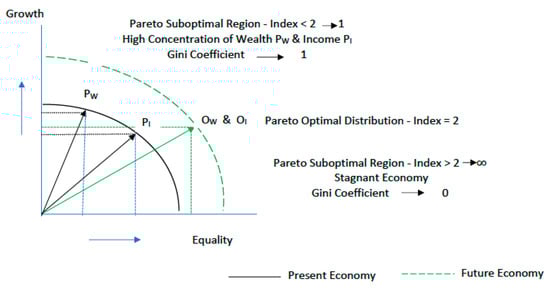
Figure 1.
Schematic graph of growth vs. equality of an economic system at the present time, where the level of growth results in high concentrations of wealth and income to fewer actors and of a future level of growth resulting in an optimal distribution of wealth and income among all the actors.
The natural question arises as to how policy makers should go about in the economic system to affect changes that would result in the optimal distribution of wealth and income. As we have discussed already, ensuring equal access to all the actors in the economic system is the necessary condition to attain optimal distribution in wealth and income. As we also have discussed, education, health care, and housing are key elements for equal access. To this list we can add the quality of infrastructure such as transportation (roads, rail, terminals), communication (universal internet and phone access), and energy (power grid, pipelines). All these sectors of the economy should be organized to function outside a for-profit structure with government involvement as well as citizen participation (Piketty, 2024; Susskind, 2024). A relevant question is how economic growth is attained and, most importantly, how it can be harnessed toward certain objectives such as the optimal distribution of wealth and of income being obtained. There are several purportedly fundamental reasons to explain inequality based on geography (physical location), culture (work ethic, enlightenment, liberalism, social capital), and institutions (rules of the game in society) (Susskind, 2024). The institutional explanation is presently the most prevalent one, although, in our opinion, all these explanations and others still to be articulated play a role with varied degrees within a particular economic system. However, and as we have already discussed, institutional constraints and reforms would be also necessary to attain equal access of the actors in the economic system. Along these lines, it is instructive to note that Daren Acemoglu and James Robinson, winners of the 2024 Nobel Prize in Economics, have drawn the distinction between extractive institutions, which allow a few actors to extract financial and material resources from the many actors in the economic system, and inclusive institutions, which provide equal access to all actors (Acemoglu & Robinson, 2012). This is exactly then, i.e., inclusive institutions, what would be conceptually necessary to be implemented to obtain the optimal, albeit still unequal, distribution of wealth and of income among the members of the economic system.
In concluding this section, we briefly address two analytical models of economic growth: the exogenous model advanced by Robert Solow and Trevor Swan and the endogenous model advanced by Robert Lucas and Paul Romer (Chirwa & Odhiambo, 2018) (Susskind, 2024). The exogenous model suggests that the primary diver of economic growth comes from external factors outside the economy such as technological progress. Growth is not the result of using more resources but the result of using those resources in a more productive way. The endogenous model argues that growth is primarily driven by internal forces within the economy such as investment in human capital, research and development, and innovation. Human capital does not refer to labor but rather to ideas originating from human beings that then can be used by anybody else. Thus, ideas are nonrival, unlike physical objects, are cumulative by their nature, as they can be reused and improved by others, and are infinite in the sense of the possible ways they can be organized and applied. Consequently, more ideas imply “not constant returns”, as with the use of physical resources, but rather “increasing returns”, such that the Malthusian problem of diminishing returns is addressed permanently.16 We should note that the scale-free network model of the economy is consistent with the endogenous model of the economy. This is so because, by virtue of its nature, the scale-free model of the economy supersedes the essentially classical in nature cause-and-effect exogenous model to use the physics analogy. Instead, the scale-free model of the economy represents the essentially infinite quantum world of ideas and resulting actions similar in nature to the basis of the endogenous model.
7. Conclusions and Recommendations
This work follows on a previous work of ours to represent an economic system as a scale-free complex network and, more specifically, to elucidate from a theoretical or analytical point of view whether there exist intrinsic differences in the empirically observed degree of wealth inequality versus income inequality. The scale-free network model of the economy is justified on the empirical observation that wealth and income distributions follow a power law. Scholarship in the past quarter century has demonstrated that systems obeying power laws such as the web can be represented by scale-free complex networks. However, we have been the first to the best of our knowledge to represent an economic system as a scale-free network comprising nodes (actors in the economic system) and links (level of wealth or income by an actor). Moreover, scholarship has also established that scale-free complex networks can be modeled analytically on the basis of statistical mechanics or thermodynamics principles. Thus, the equilibrium state of a scale-free network system is obtained when the entropy reaches a maximum value based on certain constraints characterizing the system under consideration. In an economic system, such a constraint would be the available total wealth or total annual income to be allocated among its members (actors) whose number can be fixed or variable as an additional constraint. A most critical assumption or, for that matter, constraint in the economic system as a scale-free network following the laws of statistical mechanics is that all actors have equal access to the available wealth or income, a requirement imposed in quantum physics by the indistinguishability of the members (particles) comprising the physical system, unlike classical physics, where all particles are assumed to be distinguishable.
The description of the economic system as a scale-free complex network and the subsequent derivation of a power law from first principles does not differentiate between wealth and income such that the derived power law exponent, i.e., the Pareto index, is the same for wealth as it is for income. Moreover, the scale-free network model predicts an optimal value for the Pareto index of two. Optimal here refers to the state of the distribution of wealth and of income that is the most equitable, albeit still unequal, among its members. This optimal state could be likened to what economists describe as Pareto optimality, but it occurs only at the particular value of the Pareto index of two rather than at an indeterminate value of the Pareto index. We should also note along these lines that other researchers have independently established that the numerical value of two is attained for the power law exponent of scale-free networks where all attachments among nodes (actors) are preferential and none is random. Likewise, empirical data suggest that known scale-free networks, the world-wide web being the most prominent one amongst them, have a power law exponent approaching two. Returning to the model of the economy, we note that the optimal Pareto index of two results in a corresponding optimal value of the Gini coefficient of 0.333—the Gini coefficient is directly related to the Pareto index through the Lorentz curve. Empirical evidence based on the Gini coefficient of an economy calculated from available economic data suggests otherwise. The Gini coefficients for both wealth and income are typically higher than the optimal value—the corresponding Pareto indexes are lower than the optimal value. In addition, the consensus among policy-makers and certain economists has been that the Gini coefficient occurring in an economy for wealth and for income ought to be reduced via several measures such as taxation and payment transfers. These measures aim to bring the Gini coefficient as close to zero in the erroneous belief, as the scale-free model of the economy has demonstrated, of attaining an equitable distribution of wealth and of income in the economy among all its members. In other words, the natural outcome of the distribution of wealth and of income would never lead to equal wealth and income for all the members of the economic system. Consequently, the attempt by policy-makers to obtain equal outcomes cannot succeed. On top of that, such attempts lead to the ineffective use of scarce monetary resources. A better approach would be to ensure that actors in the economic system have equal access to it. The scale-free network model of the economy indicates that an equal opportunity is the best we can strive for and for obtaining the most optimal, albeit still not equitable, distribution of wealth and of income.
Obviously, the observed inequality in the distribution of income and particularly wealth is well beyond what one would expect if equal access was in place. In attempting to elucidate if any intrinsic factors, i.e., factors not controlled by society, were at play, we developed an analytical model of the Pareto index based on the results of our model of the economy as a scale-free network and also considering the facts that (a) a general network model is essentially a system described by graph theory and (b) the network model of the economy is constrained by the laws of statistical mechanics or thermodynamics. A key parameter of a network according to graph theory is the average number of links per node. In our economic model, this parameter would represent the average wealth or income per actor, where the wealth and income are described as multiples of the quantum of wealth and of income, respectively. The existence of the quantum of wealth or of income is a critical parameter in our economic model of the scale-free network obeying the laws of quantum statistical mechanics where the existence of the quantum of energy ushered us into quantum physics.17 While in the development of our economic model of the scale-free network, the quantum of wealth or income was introduced to represent a unit of currency, we have now refined the concept to represent the minimum amount of wealth or of income an actor in the economic system can possess—this can be a multiple of the unit of currency. Thus, actors in the economic system with zero wealth or income will have zero links attached to them and would be analogous to being in the ground energy state of the physical system awaiting to be lifted to an excited state. However, our economic model as well as a scale-free network or a gas of quantum particles does not consist of a fixed number of actors, nodes, or particle energy levels, whereby such entities are allowed to enter or depart the system under consideration in a dynamically evolving system toward maximum entropy. As it turns out, the inverse of the average wealth or average income per actor in the economic system is equal to the product of the so-called “beta” parameter times the quantum of wealth or of income. This product features prominently in our model of the economy; it ranges in value asymptotically from zero to infinity and has a well-defined value of about 0.69 when the Pareto index attains its optimal value of 2. Incidentally, the so called “beta” parameter obtains its name from its counterpart parameter in statistical mechanics, where it describes the inverse of the temperature of a physical system.
The association of the economic system to a scale-free complex network that behaves in accordance with the laws of statistical mechanics leads us to consider heuristically that the Pareto index would follow a Boltzmann distribution as a function of the product of the beta parameter times the quantum of wealth or of income under the constrains that its value would range asymptotically from one to infinity and would attain the optimal value of 2 at or near the aforementioned value of “beta” times the quantum of wealth or income. An inverse or decaying exponential function is thus obtained. We note that we have now a Pareto index for wealth and a Pareto index for income. However, this distinction is not intrinsic to the economic model as a scale-free complex network but rather reflects the observed empirical distinction between the quantum of wealth and that of income. As for the values of the quantum of wealth and of income in an economic system, we have opted to use the median wealth and median income per capita to describe these values in that economic system. We have also introduced and derived the economic system temperature for wealth and for income, both expressed in units of currency and currency per year, respectively. Lastly, for comparisons of all these parameters between national economic systems, one should use exchange rates based on purchasing parity power rather than market exchange rates. We have applied these concepts to the four largest economies in the world, i.e., USA, Germany, Japan, and China. We have obtained self-consistent results with a few exceptions pertaining to China, the latter being most likely due to the quality of available data for that economy. We should also point out that none of these countries is near the optimal distribution of wealth, Japan being the closest one due to prevailing inheritance laws, while both Germany and Japan are essentially at the optimal distribution of income, which is attributable to prevailing societal conditions that ensure nearly equal access to the members of their respective economies.
The introduction of the average wealth and income per actor in the economic system as well as of the quantum of wealth and of income along with the development of a simple analytical expression to calculate the Pareto index for wealth and for income allows for a better appreciation, in our view, of the degree of inequality in the distribution of wealth and income with that economic system, which up to now is described by just the Gini coefficient. This increased appreciation, which, in turn, can provide more detailed information regarding the progress in the effectiveness of measures applied to ensure equal opportunity, is due to the increased granularity of the new parameters introduced naturally through the scale-free network model of the economy vis-à-vis the traditional Gini coefficient. The Gini coefficient, of course, remains as a paramount indicator of inequality, but our economic model provides a more expansive, more nuanced, and hopefully easier-to-comprehend degree of the existing inequality. Future research should focus on conclusively demonstrating that Pareto optimality occurs only when the Pareto index of two is attained for wealth and for income. Moreover, new parameters such as the average wealth and income, the quantum of wealth and of income, and the temperature of the economic system should enter the lexicon of metrics of the economy to track in a transparent and easily understood fashion the progress toward the objective of equal access and opportunity.
An important corollary of our work also confirms that the higher degree of inequality observed between wealth and income is not the result of any intrinsic difference in their nature and must be therefore the result of external factors imposed by the actors in the economic system. A cursory examination of public investment in education and the cost associated with health care in a for-profit environment can exacerbate inequality. Many economists have suspected this to be true, and our work demonstrates conclusively this realization. Fixing, of course, this problem will not be easy, but the overarching solution is to ensure every actor in the economic system has equal access to it, i.e., has equal opportunity. Access to quality education, health care, and housing along with equitable laws and regulations are key institutional elements in need of structural change such that all the actors in the economic system attain equal opportunity for the most equitable distribution of wealth and of income possible within the society.
Funding
This research received no external funding.
Data Availability Statement
All data employed in this work have been obtained from public sources as shown in the list of references.
Conflicts of Interest
Author Dr. John G Ingersoll was employed by the company ECOCORP INC. The remaining author declares that the research was conducted in the absence of any commercial or financial relationships that could be construed as a potential conflict of interest.
Notes
| 1 | In quantum mechanics, similar particles, say, electrons, are indistinguishable from one another. This feature is contrary to the presumed distinguishability of similar particles in classical features and is an essential characteristic of quantum particles allowing the explanation of condensation among other natural phenomena. |
| 2 | Typographical errors were discovered in Equations (30b) and (42) in the reference (Ingersoll, 2024) after the article was printed. These errors have been corrected accordingly, as shown in Equations (6) and (7). |
| 3 | The ratio of the sum of the exponential integral functions 2(nβh))/1(nβh)) converges rather slowly, such that the calculated value of (βh) of 0.67 is approximately correct. In the original reference (Ingersoll, 2024), a value of 0.664 was obtained employing less accurate numerical tables for the exponential integral functions. In any case, the exact value of (βh) for δ =2 is not critical for the purposes of this work. |
| 4 | The Pareto index for the global economy has been calculated based on a Gini coefficient of 0.65 as of 2013. |
| 5 | Graph theory as a mathematical discipline that owes its origin to a problem posed to and solved by Leonhard Euler in 1736. The problem known as the “Königsberg Seven Bridges” entailed whether one person could walk across the seven bridges connecting Kneiphof island in the middle of the river Pregel traversing the city of Königsberg in eastern Prussia and never cross the same bridge twice. Euler proved that such a path did not exist and inadvertently started a branch of mathematics known as graph theory. |
| 6 | The name for the power law exponent is typically referred to as the scale-free index for any scale-free network, and the Pareto index in the scale-free network refers to an economic system. As already indicated, the letter γ has been used traditionally to describe the scale-free index, and we have used the letter δ to describe the scale-free index or Pareto index in the model of the economy. |
| 7 | As discussed in Lynn et al., 2024, several attempts have been made by numerous investigators since the development of the original scale-free network model by Barabási & Albert, 1999, to address these issues. However, these attempts have relied on artificially imposed conditions such as global design choices for the optimization, fitness, and connectivity functions. |
| 8 | For a physical system, the proportionality constant in Equation (21) would be equal to the inverse of the Boltzmann constant kB. However, in the economic system, such a constant does not exist and is instead replaced by h, the quantum of wealth or energy. |
| 9 | It is tempting to characterize the status of an economic system at a high temperature as what these days is termed as crony-capitalism and the status of an economic system at a low temperature as socialist or even communist. |
| 10 | The most recent (2023) median wealth data for China are given per adult, and since we have been using numbers per living person, we had to modify the data by the ratio of the adults at 1.116 billion to the population of 1.409 billion (Global Wealth Databook UBS, 2023; Demographics of China, 2023). The most recent (2023) median income data for China refer to disposable income and indicate a ratio of 0.842 between the respective median and average values (National Bureau of Statistics of China, 2024b). Since in our analysis we are using gross income rather than disposable income, we have obtained the published value of the average gross income at RMB 88,807 and multiplied it by 0.842 to obtain the median gross income of RMB 74,775 (National Bureau of Statistics of China, 2024a). |
| 11 | The data on wealth and income for China show a different pattern from those from the USA, Germany, and Japan. This may be due to the quality of the available data as already alluded. Thus, the TESw should be around USD 400,000 and the TESi should be around USD 50,000 for China. |
| 12 | There are about 50 million students in primary and secondary education and almost 20 million in higher education in the USA. The resulting average expenditure by public sources is about USD 11,000 per student in primary and secondary education and about USD 37,000 per student in higher education. |
| 13 | According to Thomas Piketty, the public investment in France results in the top 10% of students received an average of EUR 250,000 to 3,000,000 for their education (all years), the middle 40% of the students received EUR 100,000, and those in the bottom 50% received EUR 60,000 to 70,000 in educational funds. The disparity in educational spending between the top 10% and the bottom 50% is roughly EUR 200,000. Given that those students who receive the most income belong to a more privileged social stratum, the public spending on education reinforces existing inequalities substantially. The differential of EUR 200,000 is about the size of the average inheritance for those in the privileged class and comes as a gift to them from the public expenditures. |
| 14 | The current average per person expenditure for health care in the USA is about USD 13,500, while the corresponding nominal figures (PPP-adjusted) are about USD 6300 (USD 7650) for Germany and USD 3650 (USD 6073) for Japan. The current life expectancy at birth in 2022 stands at 77.5 years in the USA, 81.7 years in Germany, and 84.8 years in Japan. |
| 15 | In 1963, US President John F. Kennedy made the bold claim that economic growth creates shared prosperity through one of the most famous speech lines of his presidency: “A rising tide lifts all the boats.” Thus, the myth of the “Rising Tide” was created and subsequently popularized. Recent scholarship shows otherwise. As our work shows, economic growth does not guarantee equal access to the economy by all its members, but equal access guarantees optimal distribution of wealth and of income and therefore optimal growth of the economy. |
| 16 | The Malthusian problem rests on two assumptions: (a) populations grow to take advantage of any increase in living standards; and (b) those standards become eroded over time as material resources such as food cannot keep up with the demand. A consequence of this observation is what economists call “diminishing returns.” The idea of diminishing returns expresses the reality that in producing goods and services, more inputs would increase outputs, but over time, a given input of material resources would result in a diminishing output compared to the earlier output of the same input. In the exogenous model of growth, technological innovation ensures a constant output so long as the external technological innovation remains. In the endogenous model of growth, the nonrival, cumulative, and infinite ideas ensure an increased output permanently. |
| 17 | It should be noted that the existence of the quantum of wealth and of the quantum of income, in direct analogy to energy in quantum physics, allows for an uncertainty in the total amounts of available fixed wealth and income equal to the value of the respective quanta. The implication is then, in direct analogy to quantum physics, that fluctuations in the heretofore fixed wealth and income can lead to changes in those quantities affecting the entropy and leading to a new equilibrium state. The treatment of wealth and income fluctuations in analogy to their quantum physics counterpart is beyond the scope of this article and will be addressed in subsequent work. |
References
- Abramowitz, M., & Stegun, I. A. (Eds.). (1972, December). Handbook of mathematical functions with formulas, graphs and mathematical tables. Applied Mathematic Series 55, Issued June 1964. Tenth Printing with Corrections. United States Department of Commerce, National Bureau of Standards. [Google Scholar]
- Acemoglu, D., & Robinson, J. (2012). Why nations fail. Crown Publishing, Penguin Random House. [Google Scholar]
- Adamic, L. A., & Huberman, B. A. (2000). Power-law distribution of the world wide web. Science, 287(5461), 2115. [Google Scholar] [CrossRef]
- Barabási, A.-L. (2014). Linked—How everything is connected to everything else and what it means for business, science, and everyday life. Basic Books. [Google Scholar]
- Barabási, A.-L., & Albert, R. (1999). Emergence of scaling in random networks. Science, 286, 509–512. [Google Scholar] [CrossRef] [PubMed]
- Bianconi, G., & Barabási, A.-L. (2000). Competition and multi-scaling in evolving networks. arXiv, arXiv:cond-mat/0011029. [Google Scholar]
- Bianconi, G., & Barabási, A.-L. (2001). Bose-einstein condensation in complex networks. Physical Review Letters, 86, 5632–5635. [Google Scholar] [CrossRef] [PubMed]
- Boltzmann Distribution. (2025). Wikipedia. Available online: https://en.wikipedia.org/wiki/Boltzmann_distribution (accessed on 25 October 2024).
- Bonneau, C. (2019, September). The concentration of educational investment in the US (1970–2018) with a comparison to France. Ecole Normale Superieure and Paris School of Economics. Available online: http://piketty.pse.ens.fr/files/Bonneau2019.pdf (accessed on 25 October 2024).
- Chirwa, T. G., & Odhiambo, N. M. (2018). Exogenous and endogenous growth models: A critical review. Comparative Economic Research, 21(4), 63–83. [Google Scholar] [CrossRef]
- Deaton, A. (2013). The great escape—Health, wealth, and the origins of inequality. Princeton University Press. [Google Scholar]
- Demographics of China. (2023). Wikipedia. Available online: https://en.wikipedia.org/wiki/Demographics_of_China (accessed on 30 October 2024).
- DESTATIS. (2019). Household projections in Germany. German Federal Statistical Office. Available online: https://www.destatis.de/EN/Themes/Society-Environment/Population/Households-Families/Tables/projection-household.html (accessed on 22 October 2024).
- Deutsche Bundesbank. (2023, April). Household wealth and finances in Germany: Results of the 2021 household wealth survey. Deutsche Bundesbank Monthly Report. Deutsche Bundesbank. [Google Scholar]
- Feynman, R. (1998). Statistical Mechanics—A Set of Lectures (p. 6). Westview Press—A Member of the Perseus Group. [Google Scholar]
- Gao, X. (2022). The mathematics of the ensemble theory. Results in Physics, 34, 105230. [Google Scholar] [CrossRef]
- Gao, X., Gallicchio, E., & Roitberg, A. (2019). The generalized boltzmann distribution is the only distribution in which the Gibbs-shannon entropy equals the thermodynamic entropy. The Journal of Chemical Physics, 151(3), 034113. [Google Scholar] [CrossRef] [PubMed]
- Garcia, E., & Weiss, E. (2017, September). Education inequalities at the school starting gate—Gaps, trends, and how to address them. Economic Policy Institute. Available online: https://www.epi.org/publication/education-inequalities-at-the-school-starting-gate/ (accessed on 28 October 2024).
- Global Wealth Databook UBS. (2023). Global wealth databook—Leading perspectives to navigate the future UBS 15 August 2023 (H.-F. Natalie, Ed.; pp. 119–122). Credit Suisse AG. Available online: https://www.ubs.com/global/en/family-office-uhnw/reports/global-wealth-report-2023/_jcr_content/mainpar/toplevelgrid_5684475/col2/linklistnewlook/link_copy.0357374027.file/PS9jb250ZW50L2RhbS9hc3NldHMvd20vZ2xvYmFsL2ltZy9nbG9iYWwtZmFtaWx5LW9mZmljZS9kb2NzL2RhdGFib29rLWdsb2JhbC13ZWFsdGgtcmVwb3J0LTIwMjMtZW4ucGRm/databook-global-wealth-report-2023-en.pdf (accessed on 30 October 2024).
- Goodman-Bacon, A. (2021, April). The myth of the rising tide—Economic Growth does not guarantee inclusion, but ensuring inclusion can lead to growth. Federal Reserve Bank of Minneapolis. Available online: https://www.minneapolisfed.org/article/2021/the-myth-of-the-rising-tide (accessed on 28 August 2025).
- Greenberg, M., & Gao, H. O. (2024). Twenty-five years of random asset exchange modeling. The European Physical Journal B, 97, 69. [Google Scholar] [CrossRef]
- Gut Leben in Deutschland. (2013). Gini coefficient of wealth in EU-15—Well being in Germany. Available online: https://www.gut-leben-in-deutschland.de/indicators/income/gini-coefficient-wealth/ (accessed on 23 October 2024).
- IMF GDP Nominal. (2024). IMF list of countries by GDP nominal. Wikipedia. Available online: https://en.wikipedia.org/wiki/List_of_countries_by_GDP_(nominal) (accessed on 29 October 2024).
- IMF GDP PPP. (2024). IMF list of countries by GDP PPP. Available online: https://en.wikipedia.org/wiki/List_of_countries_by_GDP_(PPP) (accessed on 29 October 2024).
- Ingersoll, J. G. (2024). Inequality in the distribution of wealth and income as a natural consequence of the equal opportunity of all members in the economic system represented by a scale-free network. Economies, 12, 232. [Google Scholar] [CrossRef]
- Lynn, C. W., Holmes, C. M., & Palmer, S. E. (2024). Emergent Scale-free networks. PNAS Nexus, 3, 236. [Google Scholar] [CrossRef] [PubMed]
- Mandelbrot, B. B., & Hudson, R. L. (2006). The misbehavior of markets—A fractal view of financial turbulence. Basic Books. [Google Scholar]
- Mantegna, R. N., & Stanley, H. E. (2000). Introduction to econophysics—Correlations and complexity in finance. Cambridge University Press. [Google Scholar]
- National Bureau of Statistics of China. (2024a). Households’ income and consumption expenditure in 2023. Available online: https://www.stats.gov.cn/english/PressRelease/202402/t20240201_1947120.html#:~:text=Among%20them%2C%20the%20median%20of,was%2086.4%20percent%20of%20the (accessed on 23 October 2024).
- National Bureau of Statistics of China. (2024b, February 29). Statistical communique of the People’s Republic of China on the 2023 national economic and social development. Available online: https://www.stats.gov.cn/english/PressRelease/202402/t20240228_1947918.html#:~:text=The%20gross%20national%20income%5B3,percent%20over%20the%20previous%20year (accessed on 30 October 2024).
- National Health Expenditure Accounts. (2024). Centers for medicare and medicaid services. Available online: https://www.cms.gov/data-research/statistics-trends-and-reports/national-health-expenditure-data/historical#:~:text=The%20data%20are%20presented%20by,spending%20accounted%20for%2017.3%20percent (accessed on 5 November 2024).
- Newman, M. E. J. (2006). Pareto laws, Pareto distributions and Zipf’s law. arXiv, arXiv:04120004v3. Available online: https://arxiv.org/PS_cache/cond-mat/pdf/0412/0412004v3.pdf (accessed on 22 August 2024).
- Nippon.com. (2024). Your doorway to Japan, one in three Japanese households consists of just one person. Available online: https://www.nippon.com/en/japan-data/h02059/ (accessed on 23 October 2024).
- Nobel. (2024). The Sverige Riksbank prize in economic science in memory of Alfred Nobel 2024. Press Release. Available online: https://www.nobelprize.org/prizes/economic-sciences/2024/press-release/ (accessed on 14 October 2024).
- OECD. (2024). OECD better life index Japan. BLI Data Base. Available online: https://www.oecdbetterlifeindex.org/countries/japan/ (accessed on 23 October 2024).
- Okun, A. (1975). Equality and efficiency: The big tradeoff. Brookings Institution Press. [Google Scholar]
- Pareto, V. (1925). Écrits sur la courbe de la répartition de la richesse (L. Droz, Ed.). Œuvres complètes: T. III. Available online: https://shs.cairn.info/ecrits-sur-la-courbe-de-la-repartition-de-la-riche--9782600040211?lang=fr (accessed on 22 August 2024).
- Pareto Distribution. (2025). Wikipedia. Available online: https://en.wikipedia.org/wiki/Pareto_distribution (accessed on 14 July 2025).
- Pareto Principle. (2024). Available online: https://en.wikipedia.org/wiki/Pareto_principle (accessed on 22 August 2024).
- Piketty, T. (2024). Nature, culture, and inequality—A comparative and historical perspective. Other Press. [Google Scholar]
- Redner, S. (1998). How popular is your paper? An empirical study of the citation distribution. The European Physical Journal B, 4, 131–134. [Google Scholar] [CrossRef]
- Schrödinger, E. (1944/1989). Statistical thermodynamics. Dover Publications, Inc. (unabridged and unaltered republication of the 2nd edition (1952) of the work first published by Cambridge University Press in 1944). [Google Scholar]
- Statista JP. (2024). Statista: Average number of members per private household in Japan 2011–2023. Available online: https://www.statista.com/statistics/606191/japan-members-per-household/ (accessed on 23 October 2024).
- Statista USA. (2024). Resident population of the United States by age and sex as of July 1, 2023. Available online: https://www.statista.com/statistics/241488/population-of-the-us-by-sex-and-age/ (accessed on 22 October 2024).
- Susskind, D. (2024). Growth—A history and a reckoning. The Belknap Press at Harvard University Press. [Google Scholar]
- The Commonwealth Fund. (2023). U.S. health care from a global perspective, 2022: Accelerating spending, worsening outcomes. Available online: https://www.commonwealthfund.org/publications/issue-briefs/2023/jan/us-health-care-global-perspective-2022 (accessed on 1 November 2024).
- Thermodynamic Beta. (2025). Wikipedia. Available online: https://en.wikipedia.org/wiki/Thermodynamic_beta (accessed on 22 October 2024).
- Trudeau, R. J. (1993). Introduction to graph theory. Dover Publications.
- United States Census Bureau. (2023a). Income in the United States: 2022. U.S. Department of Commerce. Available online: https://www.census.gov/library/publications/2023/demo/p60-279.html (accessed on 22 October 2024).
- United States Census Bureau. (2023b). The wealth of households: 2022. U.S. Department of Commerce. Available online: https://www.census.gov/content/dam/Census/library/publications/2023/demo/p70br-183.pdf (accessed on 22 October 2024).
- Unites States Census Bureau. (2024). Quick facts United States. U.S. Department of Commerce. Available online: https://www.census.gov/data/tables/time-series/demo/families/households.html (accessed on 21 October 2024).
- United States World Bank Development Indicators. (2024). United States—public spending on education, total (%GDP) 2011–2013. Available online: https://tradingeconomics.com/united-states/public-spending-on-education-total-percent-of-gdp-wb-data.html#:~:text=Government%20expenditure%20on%20education%2C%20total,compiled%20from%20officially%20recognized%20sources (accessed on 31 October 2024).
- World Bank Group. (2023). Gini index—All countries and economies. Available online: https://data.worldbank.org/indicator/SI.POV.GINI (accessed on 23 October 2024).
- Xie, Y., & Jin, Y. (2015). Household wealth in China. Chinese Sociological Review, 47(3), 203–229. [Google Scholar] [CrossRef] [PubMed]
- Zwillinger, D. (2012). CRC standard mathematical tables and formulae. CRC Press/Taylor & Francis Group. [Google Scholar]

Disclaimer/Publisher’s Note: The statements, opinions and data contained in all publications are solely those of the individual author(s) and contributor(s) and not of MDPI and/or the editor(s). MDPI and/or the editor(s) disclaim responsibility for any injury to people or property resulting from any ideas, methods, instructions or products referred to in the content. |
© 2025 by the author. Licensee MDPI, Basel, Switzerland. This article is an open access article distributed under the terms and conditions of the Creative Commons Attribution (CC BY) license (https://creativecommons.org/licenses/by/4.0/).