Abstract
In recent years, the global economy has been hit by a sequence of severe shocks that affected the two largest economies, the USA and the Euro Area, severely. Uncertainties about the future abound. While the challenges are similar for both economies and the policy tools resemble each other, they apply to different economic landscapes. What can they learn from each other? This paper looks at the basic structural facts, the nature of uncertainty shocks, and the efficiency of policy tools in the two economies. The key to understanding recent developments is uncertainty. This paper argues that the channel through which uncertainty influences inflation, wage cost, and unemployment is the markup firms charge to cover their cost of capital. While the measurements of uncertainty are uncertain, adding a proxy for uncertainty can improve the estimates of the basic New Keynesian model. The Federal Reserve Bank has been more successful because it operates in a more integrated capital market. In the Euro Area, uncertainty is higher than in the US and this could make disinflation in Europe more painful in terms of unemployment.
1. Introduction
There can be little doubt that uncertainty has increased significantly in recent years. Geostrategic considerations are ripping globalisation apart, domestic politics are becoming uncompromising, climate change is undermining living conditions, and migration seems out of control. Economic growth has been hit by major crises, and inflation is on the rise. In response to a sequence of severe shocks—from the global financial crisis, to COVID and the Ukraine occupation—fiscal authorities have run large deficits and unconventional monetary policy has swamped banks with liquidity. While this may have helped to avoid major recessions, it has also undermined trust that central banks will meet their inflation targets, and the anchor for stable inflation expectations has shifted.
Even if the economic landscapes differ, the shocks and challenges are similar in Europe and America and their policy tools for remedying the situation resemble each other. Despite some subtle differences, the economies in the United States and the Euro Area not only have identical inflation targets, but they have also performed surprisingly similarly. Treating the Euro Area as a single market and comparing it to the US can provide new insights in understanding the two economies.
A common explanation for the recent inflation surge is that monetary and fiscal policies have over-reacted to a series of interacting supply and demand shocks. The initial price shocks were perpetuated by second-round effects when wages increased to compensate for the loss of real income (). This has been interpreted as renewed evidence for distributional conflicts causing inflation.1 But while second-round effects are important, explaining inflation dynamics requires the wage-setting equation to meet the price-setting equation, which depends on the markup firms add to unit labour costs.
The European Central Bank and the IMF have recently pointed to the impact of unit profits on domestic inflation.2 They have shown that “in the presence of strong increases in costs, an unchanged markup implies similarly strong increases in unit profits”.3 But with stable markups, the inflationary dynamics will depend on the cost push from wages and intermediary consumption such as energy prices. When profits per unit of output rise faster than unit labour costs, the markup is not stable, and we observe “profit inflation”. This has now attracted increasing attention as “domestic cost pressures, measured by the GDP deflator, continued to increase in the first quarter of 2023 as a result of rising unit labour costs and unit profits” (). Profit inflation has been blamed on corporate greed.4 However, the line between profit maximisation and greed is hard to draw. In this paper, I conjecture that the driver of recent inflation was not corporate greed but the general climate of uncertainty.
Price and wage setting depend on the perceptions of firms and workers about future events and how their expectations are affected by uncertainty. Economic agents hold money balances not only for transaction purposes but also as a protection against unforeseen events. Financial markets assess the price for this liquidity preference. In equilibrium, firms must charge a markup that generates the cash flow required as protection against uncertainty. Hence, the markup will be positively correlated with higher degrees of uncertainty. With constant money supply, this means nominal wages must fall, but when the central bank accommodates the demand for money, firms can increase their prices and even concede small wage increases provided that real wages fall.
The hypothesis that uncertainty affects inflation through the markup is testable. This paper looks at the effects of uncertainty for inflation in the US and the Euro Area and studies the consequences for policy making. The paper is organised as follows. In the first part, I describe the macroeconomic landscape relevant for inflation in the Euro Area and the US economy. I present first the main macroeconomic indicators, then discuss shocks and uncertainty. This will allow us in the third part to study how uncertainty has contributed to high inflation through the profit markup channel. I first show the link between markups and price rises, then evaluate the relative weight of profit and wage inflation as a function to uncertainty. I will close by evaluating the transmission channels of monetary policy. I find that the adjustment to shocks and uncertainty operates differently on both sides of the Atlantic.
2. The Tale of Two Economies
The Euro Area is an integrated economy, even if it is politically more decentralised than the United States. The status of semi-autonomous member states leads many analysts to study national economies rather than the Euro Area as a whole. However, when we focus on monetary policy, we can treat the Euro Area as a single economy.5 The economic landscapes are, of course, not the same on both sides of the Atlantic. Both economies are large and relatively closed, but they are integrated through financial markets (). The challenges they face and the policy tools they use are not very different. If uncertainty affects markups, and unit profits are one of the drivers of inflation, monetary authorities in both continental economies must react in similar ways to uncertainty shocks.
Comparing the EA and US requires comparable data. For the US, I retrieved data from the Economic Database of the St. Louis Federal Reserve (FRED), and those for the EA from the ECB or Eurostat. Markups and wage costs were calculated from OECD data. Other sources are indicated separately. The variables encompassed inflation, measured as the logarithmic difference in the consumer price indices (CPI and HCPI), and GDP deflators. Monetary policy is represented by the Federal Funds Rate for the US and the policy rate for the ECB, as well as their respective balance sheets. All the data are quarterly except for the budget deficits, which are annually. While we have long time series for the US, the European monetary union only started in 1999Q1. Where it is of interest, I have shown longer series in the graphs. For the regressions, the data set ends with 2023Q1 unless stated differently.
3. Some Basic Facts about the European and American Economies
Table 1 summarises the performance of the two economies between 1999Q1 and 2023Q1. Mean annual inflation was lower in the Euro Area, even though the standard deviation for inflation was similar. Economic growth was lower in Europe but was more volatile. This could imply that the EA was hit by more severe supply shocks, while the US economy has been subjected to demand shocks, as suggested by (), and this would require different policy responses. Unemployment was significantly higher in Europe and less volatile than in the US. Monetary and fiscal policies were more active in the US (the standard deviations were higher), but monetary policy was more, and fiscal policy less, restrictive in the US.

Table 1.
Summary statistics for the adopted variables.
3.1. Inflation, Profits, and Wages
Figure 1 shows the development of consumer price inflation in the EA and the US in a time series with monthly data until 2024. Before the global financial crisis, Europe stayed close to the 2-percent inflation target, while in the US prices crept up under the pressure of excess demand. Since then, the swings in inflation rates have been substantial. The austerity policy during the Euro crisis pushed demand and inflation below zero, but in the US, an early attempt to start quantitative tightening dampened effective demand (). Lockouts during the COVID pandemic brought inflation below zero again, but after the Russian invasion of Ukraine prices shot up. The movement was slightly delayed in Europe, but given its dependence on imported energy, more extreme. With the return to normality, inflation rates have started to decrease, but they are still above the proclaimed 2-percent inflation target.
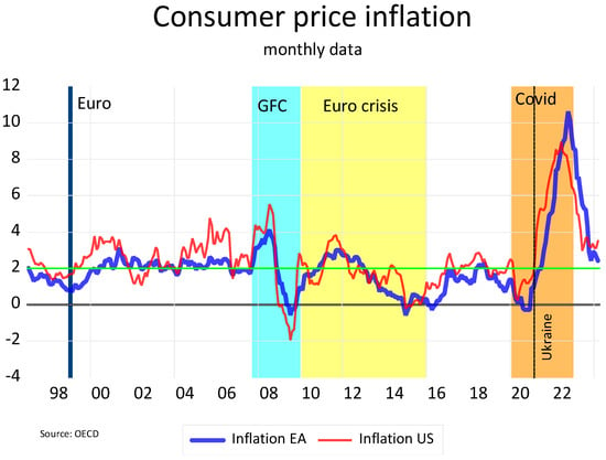
Figure 1.
Inflation in the EA and the US. The green line is the inflation target of 2%.
Yet, what matters for macroeconomic stability is not only the average performance but also the volatility around the mean. High volatility reduces visibility and creates uncertainty (), but certainty is a key variable for the effectiveness of economic policy (). It seems odd to define price stability as “inflation of 2% over the medium term” without taking account of the variance around this mean. Despite its commitment to price stability, inflation has been more volatile in the Euro Area than in the United States.
The persistence of inflation above the target undermines the credibility that central banks can deliver what they promise. () has argued that the progressive lifting of the inflation expectations anchor can be detected, first, through a right shift in the skewness of inflation distribution, then by a rise in the standard deviation, and finally by a rise in the median or mean inflation rate. Table 2 reveals that during COVID, the skewness in the inflation distribution of the Euro Area tilted significantly more to the right than in the US, and the standard deviation also rose more. This development is consistent with the observation by () that inflation uncertainty increases the level of inflation.

Table 2.
Shifting the inflation anchor.
Figure 2 shows that profit markups were always higher in Europe than in the US.6 This gap can be explained by the difference in capital productivity, which requires higher markups in less productive economies in order to remain competitive.7 The profit markups fell in Europe during the global financial crisis, but not in America, while they dropped in both economies at the outbreak of the COVID pandemic.
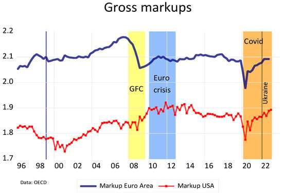
Figure 2.
The markups for the EA and the US.
It is standard wisdom that the cost of labour per unit of output (ULC) is an important element of inflation. But what about profits? They are an integral component of output prices, just like production costs, such as wages, taxes, or the cost of intermediate inputs (). I propose that the price component of profits is a function of uncertainty.
To clarify the relation between profit and wage inflation, let us start with a simple identity that describes the markup as the surplus which firms add to their unit labour costs when setting prices. Abstracting from taxes, we write the price equation as:
where is the profit margin, and the markup is
Unit labour costs are calculated as:
where is the nominal wages (compensation per employee) and is the number of employees. Productivity is the output per worker . The real unit labour costs are divided by the price level, which is effectively the wage share
This share is determined by the level of real wages relative to productivity. The markup is the inverse of the wage share and can be considered as an estimate of real marginal costs.8
It can also be shown that the profit margin is equal to the profit share relative to the wage share:
Thus, when the markup increases, the wage share falls. The tax share would reduce the profits available to firms, but given that it has been remarkably constant since the 1990s except for the COVID years, we will ignore it.
Taking the first differences of logs, we can obtain the inflation rate as follows:
The first bracket reflects the marginal markup, the second the marginal cost of labour. Rising inflation stems from markup increments and from nominal wages surpassing productivity. If the lifting of the inflation anchor primarily affected wage negotiations, we would expect increases in unit labour costs and unit profits in the same proportion. If unit profits rise more, firms generate a profit inflation; otherwise, we speak of wage inflation.
What determines the markup? Marxists believe boundless greed drives the capitalist system; there is no equilibrium. Early models assumed markups to be constant, but later their time-varying character was recognised. Models with monopolistically competitive markets interpret markup variations as reflecting the degree of monopoly power in the economy because higher competition leads to lower markups. Competition-enhancing policies would therefore structurally lower the markup ().
Alternatively, the markup can be interpreted as the outcome of competing claims on aggregate income by firms and workers (). Inflation is therefore the result of inconsistent claims and its dynamics are modelled by the wage–price spiral which settles at the equilibrium non-accelerating inflation rate of unemployment (NAIRU), See (). Thus, price stability is achieved when claims by workers and capital owners are consistent, unemployment is at its long-run natural rate, and money supply does not exceed the growth of potential output.
I conjecture that in equilibrium, firms must cover the cost of capital by their markup. The marginal cost of capital depends on the interest rate which reflects the cost of borrowing and risk assessments in capital markets. Asset owners require a compensation for the risks and discomfort of uncertainty. Because capitalism is defined by the domination of capital markets over labour markets (we do not live in “labourism”), I take the cost of capital as the forcing function for the inflationary process. The labour market must adjust, which it does either by nominal wage setting or by employment variations (the Phillips curve logic).
Deep and integrated capital markets provide opportunities for effective risk-sharing. This is essential for financing the real economy and limiting fluctuations in economic activity. However, recent ECB analysis shows that capital market integration remains rather modest (). Therefore, the transmission of monetary policy to the real economy is hampered, and this might explain why the interest channel is less efficient in Europe for bringing down inflation, as we shall see below. High financial market integration may also explain the higher activism of monetary policy by the Fed. The efficient market for Treasury bonds allows the Fed to increase interest rates quickly and strongly when required by inflationary pressures. This brings inflation expectations down across the board, so that interest rates can be lowered again. For the ECB, the market for outright monetary transactions (OMTs) is more restricted, which creates frictions for the transmissions of monetary policy that show up in the distribution of markups.
How did the relation between profit and wage inflation evolve in the US and the Euro Area? Figure 3 shows the contributions of unit labour costs, unit profits, and unit taxes to the evolution of the GDP deflator.9 Table 3 presents the balance between profit and wage inflation for different periods. A positive sign indicates profit inflation, and a negative sign wage inflation. In the USA, wage inflation always dominated profits; in the Euro Area, profit inflation was more important in the pre-crisis years 1999–2006 and in the post-COVID period. The volatility is generally higher during crisis periods. Given a negative sign for the mean, a negative (left-leaning) skewness indicates a higher likelihood that wage inflation will exceed profit inflation. In Europe, this situation prevailed during the austerity years (2007–2019), but during the early years of monetary union and during the COVID pandemic, profits were the driver of inflation. In the US, the relative impact of wage inflation was reduced during and after the global financial crisis. The kurtosis indicates that the distribution of the relative inflation components has a flatter tail, which means outliers were more frequent (). In Europe, the kurtosis was higher than in the United States during the Euro crisis and pandemic/Ukraine years. Thus, the Euro Area has suffered more from uncertainty shocks, and this would explain why inflation volatility was lower in America.
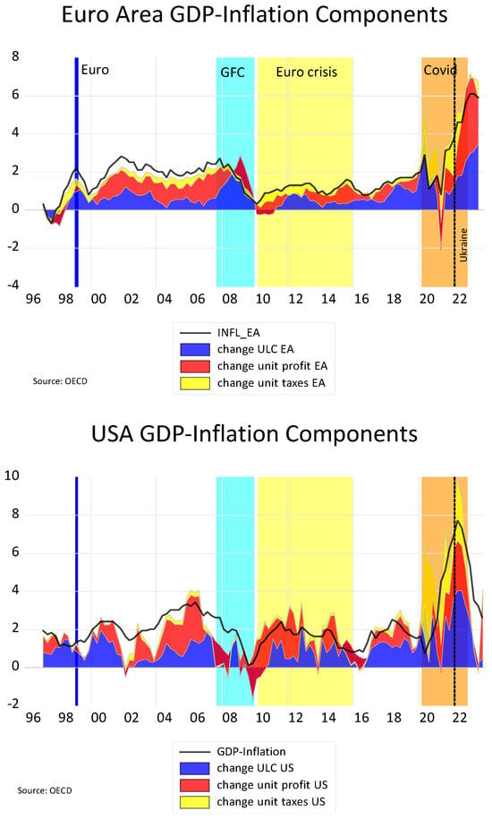
Figure 3.
Inflation components.

Table 3.
Gap between profit and wage inflation.
3.1.1. Macroeconomic Policy and Economic Growth
A notable contrast between the 1970s and the current era is the considerably larger size of the financial markets. The financial crisis in 2007 increased uncertainty and disrupted the financial sector. If uncertainty causes higher liquidity preference, central banks must increase liquidity and give priority to the short-term stabilisation of financial markets over their medium-term inflation targets. Figure 4 confirms that the ECB was less reactive than the Fed. The Fed cut rates quickly during the Great Recession, and when interest rates reached the zero lower bound it started unconventional policies and quantitative easing (; ). The Obama administration stimulated the economy with large deficits. The ECB followed the Fed’s rate decisions with delays, while fiscal policy remained restricted, and the European policy mix worsened. After ECB President Mario Draghi’s declaration that the ECB “will do, whatever it takes, to preserve the euro”10, interest rates fell close to zero (some even became negative), but quantitative easing started only in 2014 with the asset purchase programmes (). The largest expansions of balance sheets occurred in both economies during the COVID pandemic.
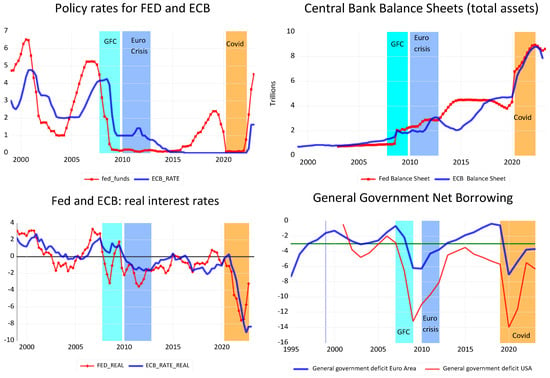
Figure 4.
Central banks’ policy rates, balance sheets, real interest rates, and general government net borrowing.
Logically, aggregate price stability would require the fall of other prices when energy prices go up, and this would require the tightening of monetary policy. In America, the central bank reacted with steep rises in interest rates, but the ECB was more timid; real interest rates are still deeply negative (see Figure 4). Nevertheless, central banks have recently started to shrink their balance sheets. This has been more pronounced in Europe.
Macroeconomic policy is conducted by two unified decision makers in the United States, the Federal Reserve System and the federal government; in Europe, only money is governed by a unified institution, the ECB. Fiscal policy is restricted by the Stability and Growth Pact and serves only in exceptional cases as a policy tool. During the pandemic, the pact’s rules were suspended and the FutureGenerationEU programme provided a stimulus. Yet, European stabilisation policies depend primarily on the ECB and this fact is causing a severe overload for the responsibility of the ECB (). Yet, surprisingly, this overload does not show as higher activism. The Fed Funds rate has varied more than the ECB policy rate and American budget deficits have been on average twice as high and twice as variable as in Europe. Hence, the US has an active macroeconomic policy approach, while the Euro Area is more passive. This has consequences for economic growth.
Figure 5 depicts the real growth rates of output for both the US and the Euro Area. The US experienced generally faster growth than the EA, which suffered particularly during the debt crisis. Thereafter, Europe shortly returned to similar growth rates before it was hit again by the COVID pandemic. Economic growth was less volatile in the USA. This may indicate that macroeconomic stabilisation policy was more successful in the United States, where monetary policy interacts with fiscal policy.
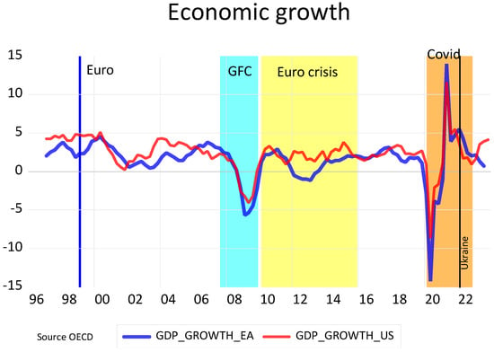
Figure 5.
The growth rate of GDP at constant prices in the EA and the US.
3.1.2. Labour Market Dynamics and the Phillips Curve
One difference between the two economies is the labour market. Distributional conflicts between profits and wages (and marginally taxes) do not determine inflation in the long run, but they matter for the level of employment. When monetary policy is accommodating, a shock to profits or wages will increase prices at a given level of activity, but when money is tight, the speed of returning to equilibrium depends on inflation expectations. Credible austerity will slow down wage and price increases, but if uncertainty about the future path of monetary policy prevails, tight money will increase unemployment, because lower profits reduce investment or because firms seek higher productivity to lower unit labour costs. This logic is reflected in the Phillips curve.
Yet, the dynamics of adjustment differs between the two continents. While inflation increased faster in America, the unemployment rate was always lower than in the Euro Area, except during the COVID crisis. In America, the pandemic had dramatic effects in the labour market, where unskilled and low-paid workers lost their jobs first (), while the European social safety net protected all employees in the Euro Area.11 Unemployment in the US peaked during the Great Recession at 10 percent, reaching European levels, but then fell again quickly below 4 percent. In Europe, it was pushed up to 12 percent by the debt crisis and then fell to 6.5 percent in 2024Q1—the lowest rate since monetary union began.
The original Phillips curve simply described the inverse statistical relationship between unemployment and wage or price increases.12 Figure 6 shows the idea (with actual and not expected inflation). () observed that the Phillips curve was non-linear,13 and () have shown that the sharp drop in core inflation in the early 1980s was mostly due to shifting long-run expectations about monetary policy as opposed to a steep Phillips curve. For the period since 2000, the European curve is flat for all unemployment rates above 8 percent, with a jump at 9.5 percent. In America, it is slightly steeper. In both countries, the curves increased significantly during the pandemic. With the war in Ukraine, the Phillips curve became vertical. We would expect that inflation would decrease quickly when unemployment rises from low levels, but not when it is permanently at high levels.
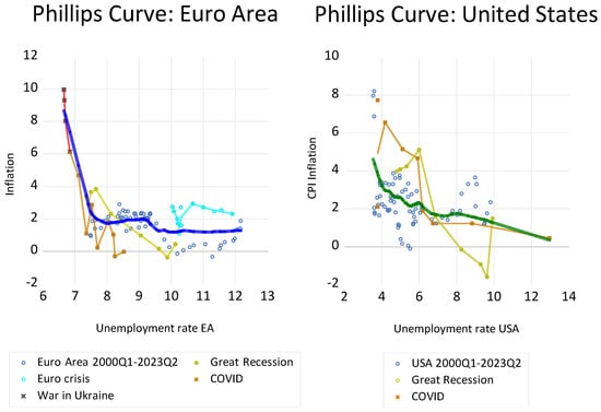
Figure 6.
Statistical Phillips curves in the two economies.
3.2. Macroeconomic Shocks, Inflation, and Uncertainty
Economic shocks are inevitable. However, their depth and frequencies have profound consequences for macroeconomic performances and inflation. Traditionally, the literature focuses on supply and demand shocks, but there is now a growing body of papers regarding uncertainty shocks.14 After discussing uncertainty shocks, I will look in this section at volatility and evidence from the Great Moderation, and estimate the impact of transitory and persistent shocks on the US and EA economies.
3.2.1. Uncertainty Shocks
Uncertainty, risk, and volatility are closely related but distinct concepts. People are uncertain if they lack confidence in their knowledge of the state of the world of future events. They deal with this uncertainty by assigning probability distributions to different prospects, but they may be uncertain about this assignment itself. In his economic theory, Keynes has therefore distinguished between a risk premium, which is related to calculable probability, and a liquidity premium, which creates a sense of comfort and confidence when people seek to protect themselves against uncertainty.15 I will speak of generalised uncertainty to cover both aspects. Generalised uncertainty emerges from social and political conflicts, financial crises, pandemics, and wars—to give some examples.
Insofar as uncertainty affects expectations about future events, it is an ex ante concept. But volatility, denoting the size of changes in asset prices, is an ex post measure of uncertainty (). () have distinguished between macro-, micro-, and higher-order uncertainty shocks, which are all positively correlated, but macroeconomic uncertainty shocks are central because when they are high, public information—past outcomes—becomes a less informative predictor of the future relative to private information. This makes agents put less weight on public information, more weight on private information, and leads them to disagree more. Furthermore, weak macro-outcomes make highly uncertain “disaster outcomes” more likely. Uncertainties of all types move in a correlated, volatile, and countercyclical way. For this reason, I shall concentrate on macro uncertainty shocks. Kozeniauskasa et al 2018. focus on output uncertainty, but the logic applies to inflation as well.
High inflation creates uncertainty about price signals which is likely to spill over into investment, production, liquidity management, and other microeconomic decisions. () have shown that inflation uncertainty (i.e., unexpected inflation shocks) has a positive and significant effect on the level of inflation and a negative and significant effect on the output growth. However, measuring the effect of generalised uncertainty on inflation is complicated by the fact that it operates through two different channels: the liquidity preference and the risk premium channel.
In the New Keynesian model, inflation is explained by the interaction of shocks which shift the aggregate demand and supply curves. The two curves are assumed to be independent of each other and the intersection of the supply and demand curves determines the equilibrium price level for the economy. A positive demand shock (an unexpected increase in spending) will shift the demand curve to the right, so that with given supply, prices, output, and employment will increase. A negative demand shock does the opposite. By raising interest rates, monetary policy shifts the demand curve back to the left. However, this applies only to the short term. If aggregate supply is determined by the capital stock, and monetary policy affects investment, then monetary policy has hysteresis effects and the long-run effect on supply and employment depends on the duration of the shock.16 A negative supply shock, such as an uncertainty shock, will shift the supply curve to the left; given the level of demand, output and employment will fall and prices will go up (stagflation). Money supply needs to be reduced to match the lower output and facilitate the adjustment of relative prices.
When uncertainty increases liquidity preferences, firms must increase their markup to generate larger cash flows. When uncertainty increases the risk premium, it also requires higher returns on capital to cover for higher interest rates, but it will also reduce the appetite to take on new risks which translates into negative supply and demand shifts (). If the negative shift of the demand shock dominates, prices, and therefore profits, may first fall, but firms will subsequently react by increasing their markups.
Uncertainty will then pose a dilemma for monetary policy. On the one hand, with a higher liquidity preference, people wish to hold higher cash balances for contingencies. To avoid a recession, central banks must accommodate this demand for liquidity. On the other hand, if the increase in liquidity leads to higher inflation expectations, people will shift planned future spending into the present and the demand curve to the right. Inflation goes up and the expectations become self-fulfilling. However, this substitution effect can switch the slope of the demand curve. As rising prices become associated with higher output, the slope of the demand curve becomes positive. But if the inflation leads to a permanent increase in wage costs, this is a negative supply shock (shifting the supply curve to the left) which generates a lower equilibrium with an upward-sloping demand curve. () have shown that this switch in the slope of the demand curve will occur when the central bank raises interest rates less than the increase in inflation expectations. Monetary policy must avoid this behaviour by keeping inflation expectations closely anchored to the inflation target. In this case, the cost of reducing inflation in terms of growth and employment will be low (). But when the commitment to price stability weakens, inflation fears will overshoot rational expectations, and this generates more uncertainty about future inflation. Thus, uncertainty complicates the story, because by shifting both supply and demand curves to the left, it will push firms to raise their markups and therefore accelerate inflation.
3.2.2. Have Shocks Ended the Great Moderation?
When () coined the notion of the Great Moderation, he suggested three not mutually exclusive explanations for the long-run tendency of improved macroeconomic stability. First, structural changes and deeper financial markets increased the flexibility and stability of the economy. Second, the New Keynesian paradigm had improved macroeconomic policies since the 1970s (); see also (; ; ). Third, good luck also contributed to stability, as the economy was experiencing smaller and less frequent shocks. However, over the last two decades, the world has been “unlucky”, as it was hit by a sequence of serious shocks which have increased uncertainty. We find important differences in how the US and Euro Area economies dealt with these shocks.
Figure 7 reproduces and extends the indices of macroeconomic volatility developed by (). We perceive a fall of volatility during the 1950s and 60s, first for consumer prices and then for output growth, too. After the oil price shock in 1973, it took nearly 15 years to return to stability. The Great Inflation was succeeded by the Great Moderation, which lasted from the mid-1980s until the global financial crisis in 2007. After 2014, the two economies reconnected with the previous moderation trends until the COVID crisis destabilised all economies. In the Euro Area, consumer prices have nearly always been more volatile. This is puzzling, as it contradicts the ECB’s mandate of maintaining price stability. One explanation for the greater macroeconomic stability in the US may be the greater activism of monetary and fiscal policy.
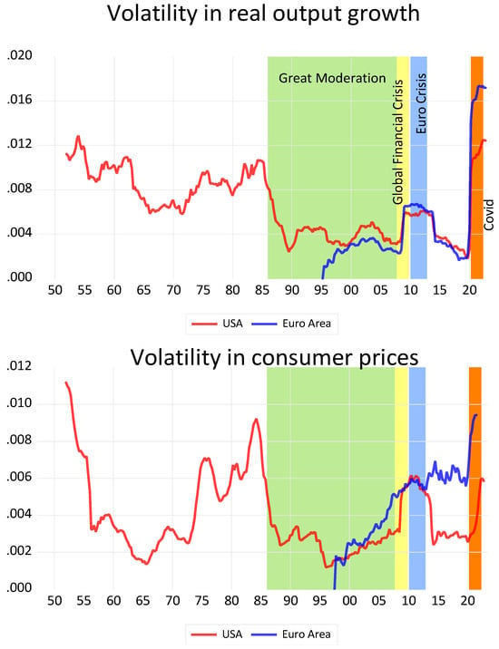
Figure 7.
The real output growth and consumer price volatility indices for the EA and the US.
Unconventional policies with zero interest rates and quantitative easing were designed to prevent major recessions caused by the global financial crisis and COVID shock. These policies deviated from the standard policy model, but they contributed to a rapid return to moderate volatility in real GDP. () found that “if the ECB had not put in place the measures adopted between 2014 and 2017, annual output growth would have been, on average, 0.67 percentage points lower in peripheral countries [of the Euro Area]”. However, the return to low price volatility was more pronounced in the USA, indicating that macroeconomic policy was less efficient in Europe.
In both economies, inflation volatility was positively correlated with variations in the central bank’s balance sheet and more so in Europe (see Figure 8). Clearly, the relation is not linear, but Figure 8 shows that low balance sheet data are correlated with low volatility and large balance sheets with high volatility. The higher response of inflation volatility to variations in the central bank’s balance sheet is a structural feature and not policy-induced. A closer look at the balance sheet of the two banks reveals that the mean growth rates of their balance sheets were similar, but the median was higher in Europe. Hence, the distribution was more skewed to the right in the USA. This means that the balance sheet expansions by the FED were generally larger, but this liquidity was subsequently reduced in smaller gradual steps.17 I interpret this as a sign that the Fed can conduct open-market operations more smoothly because the Treasury Bond market is fully integrated and liquid. Without a deep market for Euro bonds, the ECB’s open-market operations are coarser, and the consequence is higher inflation volatility. Thus, improving financial market integration would improve the macroeconomic performance of the Euro Area.
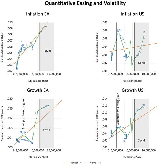
Figure 8.
Scatter plot of volatility against quantitative easing for the EA and the US.
3.2.3. Nominal and Transitory Shocks
I have argued that uncertainty shocks shift both demand and supply curves to the left. Depending on how long the uncertainty lasts, the effect will be temporary if the shock is short (such as changes in spending or inventory), but long-lasting if it generates hysteresis effects ().
() have provided a method for disentangling shocks. Yet, such shocks are econometric artefacts. The literature calls them demand and supply shocks, but because demand shocks can also have long-run supply effects, the distinction between demand and supply shocks is blurred.18 I call nominal shocks the transitory combined effect of supply and demand shocks, and real shocks the persistent combined effect. For example, a sudden increase in investment or a positive productivity shock will unambiguously increase economic growth. A protracted financial crisis, like the Euro debt crisis, will lower real GDP growth for a long time. These are therefore real shocks. By contrast, an unexpected increase in prices, profits, or unit labour cost is a nominal shock which will only have real consequences if real rigidities prevail. Thus, a shock that creates short-term uncertainty is transitory, but if uncertainty becomes a generalised view of the state of the world, it has lasting effects.
The dynamics for our two economies are shown by the impulse response functions (IRFs) in Figure 9. For both countries, real persistent shocks have a stable and statistically significant positive long-run effect on real GDP growth. We note that the reaction is higher in Europe. If we assume that the Euro Area is a portfolio of advanced and emerging economies, this is consistent with () observation that the negative response to real shocks is higher in emerging market economies than in advanced countries. Transitory nominal shocks, however, have no long-run effects on real growth, as postulated by theory. Although the impulse response looks higher in Europe, the nominal shocks in both countries are statistically not significant. Hence, temporary increases in government spending (unless they shift the supply curve) or quantitative easing are unlikely to stimulate economic growth in the long run. However, the pandemic has generated new supply-side-oriented fiscal policies. In Europe, the EUR 806.9 billion investment project called NextGenerationEU aims at concrete improvements in European infrastructure and production capacities. President Biden’s USD 1.2 trillion Bipartisan Infrastructure Law has similar intentions. These programmes diverge from traditional New Keynesian demand management by not only generating aggregate demand, but also by providing long-lasting supply enhancements for economic growth.
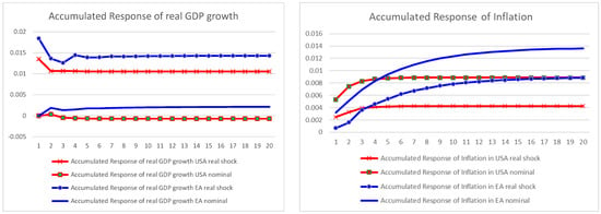
Figure 9.
The IRF plot for real and nominal shocks for the EA and the US.
However, the response of inflation to shocks is not the same in Europe and America. While in both countries real and nominal shocks increase inflation, the effects were rapid and short-lived in the USA. In Europe, they initially raised inflation less, but over time inflation increased more in the Euro Area than in the US. The inflationary response to an increase in temporary stimulus programmes was nearly twice as high in the EA as in the US. One reason could be that the US market is more competitive. This might explain why inflation moderation was higher in the US after the financial crisis when quantitative easing was effectively a nominal shock. However, these estimates indicate that policies to contain inflation and return to price stability do not work in a similar fashion in the two economies.
3.3. The Impact of Uncertainty on Inflation
The channel through which uncertainty affects prices is the markup. In equilibrium, the markup must compensate the owners of asset for risks and worries, and it will vary with the perceived degrees of uncertainty. To assess the impact, we need a measure for uncertainty. Several indicators have been created, but measuring uncertainty is still a project in its early stage.
3.3.1. Measures of Uncertainty
The most general indicator is the World Uncertainty Index (WUI), constructed for an unbalanced panel of 143 individual countries country since 1952, based on the frequency of the word “uncertainty” in the quarterly Economist Intelligence Unit (). For the Euro Area, I have calculated the WUI as the median of the national indices for the member states. Being based on media reporting, this index has the advantage of being broad and covering the full range of uncertainties occurring in the world; it has the disadvantage of not addressing specific economic risks and uncertainties.
Another set of indices measures volatility in financial market. For the United States, the Chicago Board of Options Exchange (CBOE) publishes its volatility index, called VIX. It is an options-derived series that predicts one-month-ahead volatility based on the CBOE S&P 500 futures contract (). For the Euro Area, we used the EURO STOXX 50 Volatility Index (VSTOXX), which measures the implied variance across all options of a given time to expiry.19 The VIX is based on companies in the S&P500, while the VSTOXX uses 50 European blue-chip companies. Both are ex post indicators of the expected volatility in financial markets. As they are deriving information from options trading of the stock of major companies, they are associated with changing asset prices (). If uncertainty increases, leading to higher liquidity preference and collapsing asset prices, this will negatively affect estimated aggregate markups. This seems to have occurred during the sovereign debt crisis in the Euro Area.
Another widely used indicator is the Economic Policy Uncertainty index (EPU) based on the frequency of economic words combined with “uncertainty” in American newspaper coverage (). It associates uncertainty with economic policy decisions, regulatory changes, and geopolitical events. The European index (EPU EU) is the representative average of national economic policy uncertainty in Europe. However, its original calibration on the US economy creates uncertainty regarding the index’s applicability to Europe.20
The three uncertainty proxies are shown in Figure 10. Table 4 summarises the data. The American and European indices are closely correlated, which indicates the high degree of integration across the Atlantic. The World Uncertainty Index (WUI) signals higher general uncertainty for the US (mean, median, and std dev are higher), but the indices for financial markets and economic policy are higher in Europe. The difference between these last two indices may be explained by Europe’s lower degrees of political and financial integration. The mishandling of the sovereign debt crisis for nearly seven years contributed to financial and political uncertainty in Europe. Interestingly, financial volatility decreased after the Russian invasion of Ukraine, while uncertainty increased in the other two indices. The measure for kurtosis is always larger for the USA (above 3), indicating a high probability of exceptional uncertainty, or—to put it differently—uncertainty is more uncertain in America.
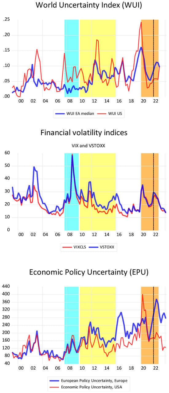
Figure 10.
Uncertainty indices.

Table 4.
Uncertainty indices 1999Q1–2024Q1.
3.3.2. Uncertainty and Profit Inflation
To test the validity of the conjecture that uncertainty causes profit inflation, I regressed each of the three uncertainty proxies on the gap between increases in unit profits and unit labour costs. If profits increase more than wages, we expect positive coefficients for these functions. As in Table 3, I define profit inflation as the positive gap between these two inflation components. The period covered was from 1999Q1 to 2023Q4. All estimates were performed with Eviews. Unit root tests (see Supplementary Materials) confirm that the time series are all stationary, although WUI EA and EPU EU are trend stationary. Granger causality exists for the WUI EU and for VIX.
I estimate two sets of models (see Table 5).21 The first six estimations show the results for dynamic autoregressive distributed lag models (ARDL) (), which allow us to combine I(1) and I(0) variables. The bound test F-statistic confirms a long-run relation between profit inflation and uncertainty in all cases. However, the long-term cointegration coefficients are only significant for the financial volatility indicators, although they have opposite signs in the two economies. In the US, the VIX index increases profit inflation, while in Europe the equivalent VSTOXX volatility increases wage inflation. Economic policy uncertainty (EPU) also has a negative coefficient for the Euro Area, but it is statistically not significant. By contrast, all other variables have positive and non-significant coefficients. Hence, with the ARDL models, the impact of uncertainty on inflation is uncertain.

Table 5.
Profit-Wage Inflation Gap 1999Q1–2024Q1.
We gain some clarity by using a VAR model. I have calculated standard and Bayesian VAR models. We assume that uncertainty induces profit inflation, but higher markups also affect uncertainty. Coincidentally, this assumption may explain why the long-run coefficients for the financial uncertainty series are significant in the ARDL model. The impulse response functions show how profit inflation responds to an uncertainty shock. For reasons of space, I only show the most interesting impulse response functions (IRFs). When the data showed serial correlation, I used the projection minimum distance operator. This method consists of minimising the distance between the data’s and the model’s impulse responses and it is not limited to linearity (). Hence, it calculates the significance of the IRF not for the aggregate time but for each moment. It appears that the WUI generates time-varying trajectories. In the first year (four quarters) after an uncertainty shock, profit inflation lags behind wage inflation but catches up in the second year. For the United States, the overall picture is clear: all three uncertainty variables have a positive impact on profit inflation. In Europe, this is less clear in the short run but confirmed for the long run, except for financial volatility, which again, as in the ARDL model, generates wage inflation. Maybe the argument of corporate greed in the distribution of conflicts has a greater impact in the European context.
The impulse-reaction functions are shown in Figure 11.
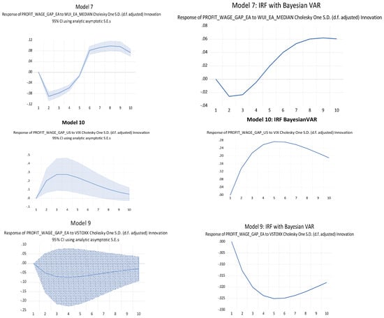

Figure 11.
Impulse response function for selected models of profit inflation.
3.3.3. Policy Effectiveness under Uncertainty
Given that we have now reasonable evidence that in most cases uncertainty increases the profit components in the GDP deflator more than the unit labour cost component, we now look at the effects of uncertainty on the overall rate of inflation. This requires placing it in the broader macroeconomic context. The standard New Keynesian model is based on three variables: prices, interest rates, and unemployment (). I have added central bank balance sheets for quantitative easing, unit labour costs to catch the markup effect, and of course, our three measures of uncertainty. First, we look at the impact of uncertainty on inflation and then how it affects the effectiveness of policy variables.
We also distinguish between long-run and short-run effects. Using level variables in logs, I have estimated Error Correction Models (ECMs) with identical specifications for the two continental economies, but with the three different uncertainty variables. Using an ECM may seem unconventional, but it is justified by the assumption that uncertainty affects inflation through the markup. A stable long-run markup implies that our variables are cointegrated, while the IRF traces the short-run adjustment dynamics. Dickey–Fuller unit root tests confirm that all variables are I(1), except for uncertainty in the US and financial volatility in Europe. Some cointegration tests suggest including a constant and a deterministic trend. The model selection uses the MacKinnon–Haug–Michaelis critical values.
Table 6 presents the estimates for the cointegrated variables. The first two columns show the benchmark models for the Euro Area and the USA without any proxies for uncertainty. According to standard New Keynesian models, we would expect the signs for interest rates and unemployment to be positive and those for quantitative easing and unit labour costs negative.22 This is not always the case. The wrong sign for ULC in Europe may be due to the existence of a long-run deterministic trend which causes the wage share to fall.23 In most cases, adding a variable for uncertainty to the benchmark model improves the results.

Table 6.
Vector Error Correction Estimates.
First, all coefficients for uncertainty are significant and have a negative sign. This means that a permanently higher level of uncertainty requires permanently higher markups. Inversely, the lesson for policy makers is that they will contribute to price stability and the perception of social equity (i.e., the absence of greed perceptions) by minimising uncertainty through stable institutions and cooperative behaviour. Second, given the long period of zero policy rates, the balance sheets of central banks (quantitative easing) have been more significant than interest rate setting. Third, an increase in unemployment rates always lowers inflation, which confirms the Phillips curve logic for the long run. Fourth, in most cases, higher permanent unit labour cost levels shift the price level up as well. In Europe, this is not the case when we have a statistically significant deterministic trend. We can, however, conclude that inflation is sensitive to second-round effects in wage bargaining. Fifth, there is a long-run deterministic trend for inflation to come down in the context of economic policy uncertainty (EPU) in both countries and with general uncertainty only in Europe (WUI EA).
Figure 12 depicts the short-run functions (IRF) of inflation responding to uncertainty in the six models. The impact of general uncertainty (WUI) on inflation is not significant in Europe or America. This is different for the variables measuring financial volatility which increase inflation in both economies. Economic policy uncertainty raises inflation in both economies, but the statistical significance is higher for Europe, probably because economic policy making is less integrated and therefore more uncertain in Europe.
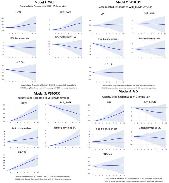
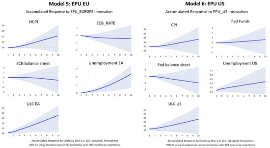
Figure 12.
Impulse response functions for different uncertainty shocks.
The response of monetary policy to uncertainty differs according to which variable we use. For general WUI uncertainty, the ECB raises interest rates but cuts them for financial uncertainty. The reaction to EPU is not significant. In the US, financial volatility leads to a cut in interest rates, but the other indicators are not significant. Quantitative easing was the response to financial uncertainty, especially in Europe, but had no significant relation with general uncertainty or economic policy uncertainty. Unemployment increases in response to policy uncertainty (EPU) in both countries, but not to general uncertainty (WUI), and only in Europe is it increased by financial markets. The same is true for unit labour costs.
Finally, in Figure 13, we inquire how uncertainty affects the efficiency of traditional policy instruments. This is revealed by the response of inflation to shocks in monetary policy and wage bargaining. I first show the two benchmark models. The US model behaves largely in line with New Keynesian theory. Higher interest rates lower inflation, while quantitative easing increases it, and so do higher unit labour costs. However, unemployment has no significant impact. This reflects the flat Phillips curve. By contrast, in the Euro Area, interest rate changes are without significant effect, but the inflationary impact of quantitative easing is significantly higher than in the US. Unemployment seems to have a larger effect in Europe but increases in ULC seem to lower inflation.
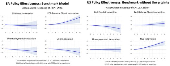
Figure 13.
Policy effectiveness benchmark models.
When we introduce the uncertainty indices, the picture does not change fundamentally but the error margins become narrower (See Figure 14). However, when central banks use variations in their balance sheets in reaction to higher volatility in financial markets, the impact on inflation is not significant. Hence, short-term financial stabilisation policies do not generate inflation. The short-run Phillips curve, whereby higher unemployment lowers inflation, is flat and insignificant in the United States but steeper in Europe.
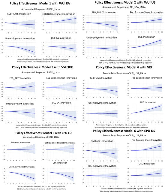
Figure 14.
Policy effectiveness models with uncertainty indicators.
4. Conclusions
This paper has studied the impact of uncertainty on the economies of the United States and the Euro Area over the last quarter of a century. We have observed a remarkable similarity in the structures and functioning of the two economies, although some differences persist. Despite a long-run tendency for macroeconomic moderation, the recent sequence of shocks and the climate of heightened uncertainty has shown some weaknesses in the functioning of the Euro Area. Although the inflation targets were met over the long run, the volatility of inflation was higher in Europe. In addition, the huge uncertainty shocks in recent years have created significant outliers. The US economy seems to absorb shocks more quickly and more smoothly. The average economic growth rate was higher in the US, most probably because of a more efficient macroeconomic policy mix, a higher degree of financial market integration, and a centralised federal government that ensures a greater degree of certitude for American economic policy. The labour markets behave differently on the two sides of the Atlantic. There is evidence for non-linear Phillips curve dynamics with stronger effects for high unemployment in Europe.
Uncertainty matters. We found that the performance of the New Keynesian model improved when we added indicators for uncertainty, although the effect was not the same for financial volatility compared to general and economic policy uncertainty. Inflation increases when uncertainty increases. In the US, this always creates profit inflation, but in Europe, volatility in financial markets and policy uncertainty create wage inflation.
What causes profit inflation is not the traditional wage–price spiral or corporate greed, but the higher risk premium that banks and financial markets demand for providing funds. The higher cost of finance requires higher markups for non-financial firms. If monetary policy remains accommodating, the adjustment to an uncertainty shock causes a temporary increase in prices, but if monetary policy remains restrictive, it will push up unemployment, which in turn will reduce wage claims in accordance with the Phillips curve logic and/or increase productivity, which lowers unit labour costs.
Anti-inflationary policies work through changes in the markup. Higher security, i.e., less uncertainty in economic policy, financial markets, and general living conditions will stabilise prices. The key to price stability is keeping a stable anchor for low inflation expectations. The Fed manages inflation expectations through the successful management of liquidity preference in the markets for Treasury bonds. The ECB does not have a similar market. Weakly integrated financial markets in the Euro Area create frictions which make the transmission of monetary policy less elastic. The Euro Area lacks a fully integrated capital market with a benchmark Euro bond which would lower the cost of capital. This pushes the burden of adjustment in Europe into the labour market. Fiscal policy is also more active in the United States. Again, Europe lacks the institutions for pursuing a coherent macroeconomic policy stance where monetary and fiscal policies interact. These two weaknesses may explain why disinflation has usually been more painful in terms of European unemployment.
Supplementary Materials
The following supporting information can be downloaded at: https://www.mdpi.com/article/10.3390/economies12070157/s1. Figure S1. Unit Roots Tests and Cointegration Tests.
Funding
This research received no external funding.
Informed Consent Statement
Not applicable.
Data Availability Statement
All data were obtained from publicly accessible sources, as explained above in the text.
Acknowledgments
I thank Yasmine Abdelfattah for her valuable research assistance and Paul de Grauwe, Sebastian Diessner, Charles Goodhart, Ben Friedman, Ricardo Reis, and Olivier Blanchard for their helpful comments.
Conflicts of Interest
The author declares no conflict of interest.
Notes
| 1 | The standard model for explaining inflation due to inconsistent wage and profit claims is the NAIRU (non-accelerating inflation rate of unemployment) model (). The assumption of a stable NAIRU implies that the two claims are stable in equilibrium. However, the acceleration in inflation is only possible if wage and price claims are accommodated by monetary policy. If money is kept tight, the consequences will be an increase in unemployment. | |||||||||||||||||||||||||||
| 2 | (; ); for the ECB and (), for IMF. | |||||||||||||||||||||||||||
| 3 | “From a firm’s perspective, this unchanged mark-up may be seen as an unchanged pricing strategy and may, in this respect, not be regarded as actively contributing to inflationary pressures, since profits are simply displaying the same strong dynamics as overall costs. However, from a macroeconomic and inflation analysis perspective, any increase in a component of a price contributes to inflation, regardless of whether there has been a change in the underlying pricing behaviour” (). | |||||||||||||||||||||||||||
| 4 | (; ; ). The frequency of the word “greed” has increased by 85 percent in Google’s ngram since the early 1990s. | |||||||||||||||||||||||||||
| 5 | (; ; ) came to the same conclusion. | |||||||||||||||||||||||||||
| 6 | Data for profit shares are from the OECD database using nominal GDP by income. | |||||||||||||||||||||||||||
| 7 | Over the 2000–2019 period, US capital productivity was on average 29% above that of the EA and the profit share in Europe 30% higher. Hence, the returns on aggregate capital were roughly equal. | |||||||||||||||||||||||||||
| 8 | () have shown that empirically, the difference between marginal cost and unit cost is not significant. () model of real marginal costs that are weighted by the capital share yield the same result. | |||||||||||||||||||||||||||
| 9 | Discrepancies are due to measurement errors and imported intermediary goods. | |||||||||||||||||||||||||||
| 10 | On 26 July 2012. For a discussion of the effects, see (). | |||||||||||||||||||||||||||
| 11 | In the United States, low-wage workers were the first to become unemployed, which led to an increase in aggregate wage compensation per worker employed (). | |||||||||||||||||||||||||||
| 12 | With the assumption of stable markups, wage and goods inflation are identical. When () introduced inflation expectations into the equation, it stopped being a description and became a short-term behavioural explanation. | |||||||||||||||||||||||||||
| 13 | See (). The New Keynesian version of the Phillips curve relates inflation expectations to the natural rate of unemployment. Modelling inflation expectations in a climate of uncertainty is itself uncertain (see below) and estimates of the natural rate of unemployment are disputed (). For the purposes of comparing the US and EA, the classical articulation is sufficient. | |||||||||||||||||||||||||||
| 14 | The early literature focussed on investment with hysteresis effects on the capital stock. See (; ). For overviews of the recent literature, see (; ; ; ). On measuring uncertainty, see (; ; ). | |||||||||||||||||||||||||||
| 15 | “I associate risk premium with probability strictly speaking, and liquidity premium with what in my Treatise von Probability I called ‘weight’. An essential distinction is that a risk premium is expected to be rewarded on the average by an increased return at the end of the period. A liquidity premium, on the other hand, is not even expected to be so rewarded. It is a payment, not for the expectation of increased tangible income at the end of the period, but for an increased sense of comfort and confidence during the period” (, pp. 293–94). Keynes’ view of risk and uncertainty therefore resembles () famous distinction. | |||||||||||||||||||||||||||
| 16 | Hysteresis refers to an event that persists even after the factors that generated it have been removed (). | |||||||||||||||||||||||||||
| 17 | Balance sheet variations 2010–2023
| |||||||||||||||||||||||||||
| 18 | () acknowledge this possibility but consider its effect negligable. | |||||||||||||||||||||||||||
| 19 | Both indices were downloaded from the FRED. | |||||||||||||||||||||||||||
| 20 | Other attempts to measure uncertainty in the Euro Area exist. () created their own economic policy uncertainty (EPU) indicators for the four largest Euro Area countries by applying two unsupervised machine learning algorithms to news articles. They observed strong negative effects of uncertainty on consumption for countries such as Italy (political) and Spain (fiscal, political, and domestic regulation). Unfortunately, I could not find an updated version. () has constructed a Euro Area integration uncertainty index (EAUI) which shows lower levels than the EPU index in recent years. Although of interest, its time series only starts in 2012 and is therefore not suitable for our analysis here. () have calculated monthly series for financial and real variables looking 3 and 12 months ahead. Providing econometric estimates of time-varying macroeconomic uncertainty, their estimates display significant independent variations from popular uncertainty proxies such as the WUI, suggesting that much of the variations in other proxies are not driven by uncertainty. Unfortunately, their index is based only on US data and there is no equivalent for the Euro Area. I will therefore discard these indices for the purpose of comparing the US and EA. | |||||||||||||||||||||||||||
| 21 | For reasons of space, I do not show the estimations, but the evidence can be obtained from the author on request. | |||||||||||||||||||||||||||
| 22 | Note that the cointegrating vector is in the form of the implicit function , so that the signs of the independent variables are negative when the variables have a long-run positive effect on inflation. | |||||||||||||||||||||||||||
| 23 | In the Euro Area, the wage share fell by 0.5 percent from 1999 to 2014. |
References
- Adam, Klaus. 2009. Monetary policy and aggregate volatility. Journal of Monetary Economics 56: 1–18. [Google Scholar] [CrossRef]
- Agarwal, Ruchir, and Miles Kimball. 2022. Will Inflation Remain High? Washington, DC: Finance and Development Magazine, IMF. [Google Scholar]
- Ahir, Hites, Nicholas Bloom, and Davide Furceri. 2022. World Uncertainty Index. NBER Working Paper. Cambridge, MA: National Bureau of Economic Research. [Google Scholar]
- Albrizio, Silvia, Iván Kataryniuk, Luis Molina, and Jan Schäfer. 2023. ECB Euro Liquidity Lines. IMF Working Papers 96. Washington, DC: International Monetary Fund. [Google Scholar]
- Alvarez, Jorge, and Allan Gloe Dizioli. 2023. How Costly Will Reining in Inflation Be? It Depends on How Rational We Are. IMF Working Paper WP 23/21. Washington, DC: International Monetary Fund. [Google Scholar]
- Andersson, Malin, Pedro Neves, and Carolina Nunes. 2023. Earnings calls: New evidence on corporate profits, investment and financing conditions. ECB Economic Bulletin Box 4. [Google Scholar]
- Ascari, Guido, Paolo Bonomolo, Marco Hoeberichts, and Riccardo Trezzi. 2023. The Euro Area Great Inflation Surge. DNB Analysis Series; Amsterdam: De Nederlandsche Bank. [Google Scholar]
- Azqueta-Gavaldón, Andrés, Dominik Hirschbühl, Luca Onorante, and Lorena Saiz. 2023. Sources of Economic Policy Uncertainty in the euro area. European Economic Review 152: 104373. [Google Scholar] [CrossRef]
- Baker, Scott R., Nicholas Bloom, and Steven J. Davis. 2016. Measuring Economic Policy Uncertainty. The Quarterly Journal of Economics 131: 1593–636. [Google Scholar] [CrossRef]
- Ball, Laurence, Gregory Mankiw, David Romer, George A. Akerlof, Andrew Rose, Janet Yellen, and Christopher Sims. 1988. The New Keynesian Economics and the Output-Inflation Trade-Off. Brookings Papers on Economic Activity 1988: 1–82. [Google Scholar] [CrossRef]
- Banerjee, Anindya, and Bill Russell. 2005. Inflation and measures of the markup. Journal of Macroeconomics 27: 289–306. [Google Scholar] [CrossRef][Green Version]
- Barrett, Philip, and Jonathan J. Adams. 2022. Shocks to Inflation Expectations. IMF Working Papers. Washington, DC: International Monetary Fund, vol. 22. [Google Scholar]
- Barro, Robert J., and Francesco Bianchi. 2023. Fiscal Influences on Inflation in OECD Countries, 2020–2022. In Tests of the Fiscal Theory of the Price Level. Unpublished manuscript. [Google Scholar]
- Bauer, Michael D., Ben Bernanke, and Eric Milstein. 2023. Risk Appetite and the Risk-Taking Channel of Monetary Policy. The Journal of Economic Perspectives 37: 77–100. [Google Scholar] [CrossRef]
- Benigno, Pierpaolo, and Gauti B. Eggertson. 2023. It’s Baaack; the Surge in Inflation in the 2020s and the Retrun of the Non-Linear Phillips Curve. NBER Working Paper Series wp 31197. Cambridge, MA: National Bureau of Economic Research. [Google Scholar]
- Bernanke, Ben. 1998. Irreversibility, uncertainty, and cyclical investment. Journal of Qarterly Economics 98: 85–106. [Google Scholar]
- Bernanke, Ben. 2004. The Great Moderation. In The Federal Reserve Board; February 29. Available online: https://www.federalreserve.gov/boarddocs/speeches/2004/20040220/ (accessed on 23 April 2023).
- Bhar, Ramprasad, and Girijasankar Mallik. 2010. Inflation, inflation uncertainty and output growth in the USA. Physica A 389: 5503–10. [Google Scholar] [CrossRef]
- Bilbiie, Florin O., and Diego R. Känzig. 2023. Greed? Profits, Inflation, and Aggregate Demand. NEBR Working Paper (31618). Cambridge, MA: National Bureau of Economic Research. [Google Scholar]
- Blanchard, Olivier. 2018. Should We Reject the Natural Rate Hypothesis? The Journal of Economic Perspectives 32: 97–120. [Google Scholar] [CrossRef]
- Blanchard, Olivier J., and Ben S. Bernanke. 2023. What Caused the US Pandemic-Era Inflation? NBER Working Paper (31417). Available online: http://www.nber.org/papers/w31417 (accessed on 25 October 2023).
- Blanchard, Olivier, and Thomas Philippon. 2003. The Decline of Rents and the Rise and Fall of European Unemployment. MIT, Unpublished paper. Available online: https://crei.cat/wp-content/uploads/2016/09/blanchard.pdf (accessed on 25 October 2023).
- Blanchard, Olivier, and Danny Quah. 1989. The dynamic effects of aggregate demand and supply disturbances. American Economic Review 79: 655–73. [Google Scholar]
- Blanchard, Olivier, and John Simon. 2001. The Long and Large Decline in U.S. Output Volatility. Brookings Papers on Economic Activity 2001: 135–64. [Google Scholar] [CrossRef]
- Bloom, Nicholas. 2009. The Impact of Uncertainty Shocks. Econometrica 77: 623–85. [Google Scholar]
- Bloom, Nicolas. 2014. Fluctuations in Uncertainty. Journal of Economic Perspectives 28: 153–76. [Google Scholar] [CrossRef]
- Born, Alexandra, Franziska Bremus, Wieger Kastelein, Claudia Lambert, and Natalia Martín Fuentes. 2022. A Deep Dive into Risk Sharing through the Capital Channel in the Euro Area—Inter- versus Intra-Regional Risk Sharing Financial Integration and Structure in the Euro Area. Frankfurt: ECB. [Google Scholar]
- Cerra, Valerie, Antonio Fatás, and Sweta C. Saxena. 2020. Hysteresis and Business Cycles. IMF Working Paper WP/20/73. Cambridge, MA: National Bureau of Economic Research. [Google Scholar]
- Dixit, Avinash, and Robert S. Pindyck. 1994. Investment under Uncertainty. Princeton: Princeton University Press. [Google Scholar]
- ECB. 2023. Economic, financial and monetary developments. Economic Bulletin 4: 2023. [Google Scholar]
- ECON Committee. 2022. 10 Years after “Whatever It Takes”: Fragmentation Risk in the Current Context Compilation of Papers. Luxembourg: European Parliament. [Google Scholar]
- Ehrmann, Michael, and Marcel Fratscher. 2002. Interdependence between the Euro Area and the US: What Role for EMU? ECB Working Paper No. 200. Available online: https://papers.ssrn.com/sol3/papers.cfm?abstract_id=376184 (accessed on 1 May 2024).
- Friedman, Milton. 1968. The Role of Monetary Policy. The American Economic Review 58: 1–17. [Google Scholar]
- Hahn, Elke. 2023. How have unit profits contributed to the recent strengthening of euro area domestic price pressures? ECB Economic Bulletin, Boxes 4. [Google Scholar]
- Hansen, Niels-Jakob, Frederik Toscani, and Jing Zhou. 2023. Euro Area Inflation after the Pandemic and Energy Shock: Import Prices, Profits and Wages. IMF Working Papers WP/23/131. Cambridge, MA: National Bureau of Economic Research. [Google Scholar]
- Hazell, Jonathon, Juan Herreno, Emi Nakamura, and Jon Steinsson. 2022. The Slope of the Phillips Curve: Evidence from U.S. States. Quarterly Journal of Economics 137: 1299–344. [Google Scholar] [CrossRef]
- IMF. 2013. World Economic Outlook. Washington, DC: International Monetary Fund. [Google Scholar]
- Istrefi, Klodiana, and Sarah Mouabbi. 2018. Subjective interest rate uncertainty and the macroeconomy: A cross-country analysis. Journal of International Money and Finance 88: 296–313. [Google Scholar] [CrossRef]
- Jordà, Òscar, and Sharon Projection Kozicki. 2006. Minimum Distance: An Estimator for Dynamic Macroeconomic Models. UC Davis Economics Working Paper. vol. No. 06-27, Available online: https://economics.ucr.edu/wp-content/uploads/2019/11/OscarJorda5-5-2006.pdf (accessed on 1 May 2024).
- Jurado, Kyle, Sydney C. Ludvigson, and Serena Ng Source. 2015. Measuring Uncertainty. The American Economic Review 105: 1177–216. [Google Scholar] [CrossRef]
- Keynes, John Maynard. 1979. The General Theory and After: A Supplement. The Collected Writings of John Maynard Keynes. London: Macmillan, vol. xxix. [Google Scholar]
- Knight, Frank H. 1921. Risk, Uncertainty, and Profit. Boston: Hart, Schaffner & Marx. Boston: Houghton Mifflin Company. [Google Scholar]
- Kozeniauskasa, Nicholas, Anna Orlik, and Laura Veldkamp. 2018. What are uncertainty shocks? Journal of Monetary Economics 100: 1–15. [Google Scholar] [CrossRef]
- Kuttner, Kenneth N. 2018. Outside the Box: Unconventional Monetary Policy in the Great Recession and Beyond. Journal of Economic Perspectives 32: 121–46. [Google Scholar] [CrossRef]
- Layard, Richard, Stephen Nickell, and Richard Jackman. 1991. Unemployment. Macroeconomic Performance and the Labour Market. Oxford: OUP. [Google Scholar]
- Lorenzoni, Guido, and Iván Werning. 2023. Inflation Is Conflict. In National Bureau of Economic Research Working Papers. Working Paper 31099. Cambridge, MA: National Bureau of Economic Research. Available online: http://www.nber.org/papers/w31099 (accessed on 7 February 2024).
- McNamara, Kathleen. 2015. The Forgotten Problem of Embeddedness: History Lessons for the Euro. In The Future of the Euro. Edited by R. Matthias Matthijs and Mark Blyth. Oxford: OUP, pp. 21–43. [Google Scholar]
- Neely, Christopher. 2021. Measuring Uncertainty and Volatility with FRED Data. FRED. June 25. Available online: https://fredblog.stlouisfed.org/2021/06/measuring-uncertainty-and-volatility-with-fred-data/ (accessed on 25 April 2024).
- Owens, Lindsay. 2022. Corporate Profits Are Soaring as Prices Rise: Are Corporate Greed and Profiteering Fueling Inflation? Washington DC: US Senate Committee on the Budget. Available online: https://www.budget.senate.gov/imo/media/doc/Lindsay%20Owens%20-%20Testimony%20-%20U.S.%20Senate%20Budget%20Committee.pdf (accessed on 7 April 2024).
- Pagliacci, Carolina. 2003. Comparing the inflationary impacts of uncertainty between advanced and emerging economies. Macroeconomics and Finance in Emerging Market Economies, 1–20. [Google Scholar] [CrossRef]
- Pagliari, Maria Sole. 2021. Does One (Unconventional) Size Fit All? Effects of the ECB’s Unconventional Monetary Policies on the Euro Area Economies. Working Paper 829. Paris: Banque de France. [Google Scholar]
- Pastorek, Daniel. 2023. Euro area uncertainty and Euro exchange rate volatility: Exploring the role of transnational economic policy. Finance Research Letters 58: 104351. [Google Scholar] [CrossRef]
- Pesaran, Hashem, and Yongcheol Shin. 1995. An Autoregressive Distributed Lag Modeling Approach to Co-Integration. Edited by ResearchGate. Available online: https://www.researchgate.net/publication/4800254 (accessed on 7 April 2024).
- Phillips, Alban W. 1958. The Relation between Unemployment and the Rate of Change of Money Wage Rates in the United Kingdom, 1861–1957. Economica, New Series 25: 283–99. [Google Scholar] [CrossRef]
- Reis, Ricardo. 2021. Losing the Inflation Anchor. Brookings Papers on Economic Activity 2021: 307–79. [Google Scholar] [CrossRef]
- Reis, Ricardo. 2023. Four Mistakes in the Use of Measures of Expected Inflation. AEA Papers and Proceedings 113: 47–51. [Google Scholar] [CrossRef]
- Rouse, Cecilia, and Martha Gimbel. 2021. The Pandemic’s Effect on Measured Wage Growth. In CEA—The White House; April 19. Available online: https://www.whitehouse.gov/cea/written-materials/2021/04/19/the-pandemics-effect-on-measured-wage-growth/ (accessed on 3 May 2023).
- Smets, Frank, and Raf Wouters. 2004. Comparing Shocks and Frictions in US and Euro Area Business Cycles. A Bayesian DSGE Approach. ECB Working Paper Series 391. Frankfurt am Main: European Central Bank. [Google Scholar]
- Stock, James H., and Mark W. Watson. 2001. Vector Autoregressions. The Journal of Economic Perspectives 15: 101–15. [Google Scholar] [CrossRef]
- Weber, Isabella M., and Evan Wasner. 2023. Sellers’ Inflation, Profits and Conflict: Why can Large Firms Hike Prices in an Emergency? University of Massachusetts Amherst Economics Department Working Paper Series 343; Amherst: University of Massachusetts Amherst. [Google Scholar] [CrossRef]
- Wellink, Nout. 2023. Crises have shaped the European Central Bank. Journal of International Money and Finance 138: 102923. [Google Scholar] [CrossRef]
- Whaley, Robert. 2009. Understanding the VIX. Journal of Portfolio Management 35: 98–105. [Google Scholar] [CrossRef]
- Yellen, Janet L. 2012. Revolution and Evolution in Central Bank Communications. In Board of Governors of the Federal Reserve System; November 13. Available online: https://www.federalreserve.gov/newsevents/speech/yellen20121113a.htm (accessed on 24 April 2023).
Disclaimer/Publisher’s Note: The statements, opinions and data contained in all publications are solely those of the individual author(s) and contributor(s) and not of MDPI and/or the editor(s). MDPI and/or the editor(s) disclaim responsibility for any injury to people or property resulting from any ideas, methods, instructions or products referred to in the content. |
© 2024 by the author. Licensee MDPI, Basel, Switzerland. This article is an open access article distributed under the terms and conditions of the Creative Commons Attribution (CC BY) license (https://creativecommons.org/licenses/by/4.0/).