Article

On the Asymmetric Relation between Inflation and Growth in Mexico: A NARDL Approach

by
José Carlos Trejo-García
,
Ramón Valencia-Romero
,
María De Lourdes Soto-Rosales
and
Francisco Venegas-Martínez
*
Escuela Superior de Economía, Instituto Politécnico Nacional, Mexico City 11350, Mexico
*
Author to whom correspondence should be addressed.
Economies 2024, 12(1), 21; https://doi.org/10.3390/economies12010021
Submission received: 18 December 2023 / Revised: 10 January 2024 / Accepted: 14 January 2024 / Published: 17 January 2024
(This article belongs to the Special Issue Fiscal Policy and Macroeconomic Stability)

Abstract

:
The effects of various geopolitical tensions, conflicts between countries and the global post-pandemic COVID-19 have caused an acceleration in the price level in many countries around the world. This research focuses on Mexico since its monetary policy has created intricate interactions between inflation and growth in the short and long term, maintaining recently one of the highest real interest rates in Latin America (on average 5.75% vs. the US 2.3%). This paper examines the asymmetric link between the National Consumer Price Index and the Global Economic Activity Index in Mexico during the period 1994–2023. To do this, a Nonlinear Autoregressive Distributed Delay (NARDL) model is used with monthly data, which will allow the relationship between both variables to be more adequately investigated. The main empirical finding is that upward or downward shocks to the consumer price index have caused different effects in magnitude and sign on economic growth over time. Finally, several reasonable, practical, and feasible recommendations are provided for the design of the monetary policy considering non-linear effects.

1. Introduction

There are many studies on how inflation negatively or positively affects economic growth (Temple 2000; Barro 1995; Fischer 1993). One of the commonly asked questions is whether inflation itself directly influences or is the uncertainty surrounding inflation that hinders or stimulates economic growth. For instance, Okun (1971) and Friedman (1977) suggest that higher inflation reduces economic growth. However, positive or negative changes do not always have the same effects and are often asymmetric (non-linear) (Kahneman and Tversky 1979; Shiller 1998).
Following the global pandemic and the conflict between Russia and Ukraine, prices rose in most economies. The causes can be on the side of supply or demand, with both positive and negative effects. Therefore, the questions here are whether inflation has any relationship with the pace of economic activity in the short and long term and whether this relationship could reflect non-linear asymmetric behavior; that is if there is an inflationary economic environment that makes the objective of monetary policy impossible and undermines confidence in the productive sector. In this sense, numerous studies have considered the problems of asymmetry (non-linearity), as well as the difficulty they generate in making robust inferences or forecasts (Kassi et al. 2019; Sowah et al. 2023; Allen and McAleer 2021).
Regarding the bibliographic gap on non-linearity, the relationship between economic growth and inflation in Latin America has been a topic of research and debate. A key literature gap revolves around the balance between these two variables. Traditionally, the Phillips curve framework suggests an inverse relationship between inflation and unemployment, implying that low unemployment (high economic growth) could be associated with higher inflation and vice versa. However, the applicability of this framework to Latin American economies, which have experienced an intricate history of high inflation and economic instability with asymmetric (non-linear) effects, has been widely questioned. Particularly in the context of inflation and economic growth, this research is an innovative approach to understand the complex dynamics of Mexico’s deep integration into the global economy as one of the two largest economies in Latin America. In some cases, the results of this type of analysis can be considered as an example with valuable insights for policymakers, academics, and economic researchers, considering the possible relationship between nonlinear models, high-frequency data, and the distinction between short- and long-term effects with the consideration of the General Index of Economic Activity (monthly data) as an alternative variable to the common Gross Domestic Product (quarterly or annual data). Therefore, this provides a new perspective on economic policymaking in Mexico with high-frequency granular data, which is especially valuable in rapidly changing economic environments when crucial decisions must be accelerated and specific policy responses are required.
On the other hand, inflation and economic growth are two crucial factors in an economy, and their interactions have been complex in the case of Mexico (Central Bank of Mexico, from now on, briefly, Banxico 2022). The monetary policy applied by Banxico has created intricate interactions between inflation and growth in the short and long term, often characterized by asymmetric effects. A proper understanding of these relationships is essential for policymakers to strike the right balance between maintaining price stability and fostering sustainable economic growth.
On the other hand, it is worth mentioning that Mexico has one of the highest real interest rates in Latin America. This shows that Mexico has a more restrictive position in the region, despite having stopped its cycle of core rate increases; therefore, expectations are that the performance of consumer prices will be able to slow down, attract capital flows, and strengthen the national currency.
For the Mexican case, this research contributes to the relevant literature on asymmetric effects in the inflation–growth nexus because very few studies have been carried out that consider periods shorter than annual measurements, such as the growth of the gross domestic product (GDP) and the inflation rate. For this, the Non-linear Autoregressive Distributed Lag (NARDL) model will be applied. This approach allows the investigation of asymmetric effects, capturing the differential impact of inflation on economic growth during periods of rising inflation compared to periods of falling inflation. In this way, a good combination of the benefits of high-frequency data analysis with the robustness of NARDL is achieved, allowing a better understanding of the intricate interactions between these variables with the finer temporal resolution, which is especially valuable in rapidly changing economic environments, where crucial decisions can speed up when more targeted policy responses are required. The originality in the research of monthly data with NARDL models is evident in the context of the Mexican case: (1) fine-tuned short-term dynamics, (2) non-linear insights, (3) timely decision-making, (4) fine-tuned policy implications, and (5) real-time monitoring.
Therefore, this research aims to examine the existence of asymmetry between economic growth rates of the monthly index of economic activity (IGAE, Spanish acronym for Índice Global de Actividad Económica) and the monthly price index (INPC, Spanish acronym for Índice Nacional de Precios al Consumidor). Monthly data for Mexico are obtained from the Mexican National Institute of Statistics and Geography, during the period 1994–2023, which will be used in a NARDL model with the consideration of short- and long-term asymmetries. Therefore, this work stands as a significant contribution to the field, highlighting its methodological rigor, extensive data analysis, and valuable policy implications, all of which collectively elevate its relevance and importance in the literature on the subject.
The rest of the investigation is organized by first analyzing the periods of economic recession due to geopolitical reasons and the global health emergency of the COVID-19 pandemic, as well as the periods of rising prices in Mexico, mentioning the facts that influenced their behavior in the face of the reactivation of consumption and economic production. Subsequently, a NARDL model will be used with the confirmation of the required econometric tests. Finally, the discussion of the empirical results and conclusions with recommendations are provided.

2. A Brief Literature Review

In recent years, many studies have delved into the complexities of NARDL models, shedding light on their ability to capture the non-linear relationship between inflation and economic growth. In this sense, Hossain et al. (2021) found asymmetry in this relationship and suggested that positive changes in inflation have a substantial short-term positive influence on growth, while negative changes are less impactful. These authors found several implications for policy implementation in Bangladesh, suggesting that moderate inflation could be beneficial for economic growth. Likewise, Chen et al. (2020) investigated the impact of financial development and prices on economic growth in Kenya using a NARDL model, finding an asymmetric relationship. Moreover, Al Khatib (2023) studied the relationship between financial development (FD) and economic growth (EG) in Syria from 1980 to 2018; this asymmetry suggests that the impact of FD on EG is complex and varies with the levels of FD, offering insights for policymaking in Syria and emphasizing the importance of creating conditions that foster positive FD shocks for long-term economic growth. Also, Ismail and Masih (2019) examined the relationship between inflation and economic growth in South Africa using the NARDL approach, showing the existence of a long-run equilibrium relationship between the two variables, providing insights into the complex dynamics of inflation’s impact on economic growth, and contributing to the broader understanding of macroeconomic stability and policy development. On the other hand, Torun (2023) examined the relationship between oil prices and economic growth in Turkey from 1976 to 2021, utilizing a NARDL model the author found that both positive and negative oil price shocks asymmetrically affect Turkey’s economic growth. This dynamic is crucial for effective economic policymaking, especially considering its dependence on oil imports and the impact of global oil price volatility on its economy. Furthermore, Ekpeyong (2023) analyzes the impact of inflation, unemployment, and economic growth on poverty in Nigeria using the NARDL approach from 1980 to 2021. The author provided insights into the relationships between these variables. Similarly, Khalili et al. (2023) investigated the impact of inflation on Iran’s economic growth using a NARDL model, highlighting that negative changes in inflation have a significant adverse effect on economic growth, while positive changes in inflation have no significant impact. Nene et al. (2022) explored the impact of inflation targeting policies on inflation uncertainty and economic growth; the study assessed the effects in selected African and European countries, finding that inflation targeting policy significantly reduces inflation uncertainty in European countries and has a positive impact on their economic growth. Olamide et al. (2022) examined the effects of exchange rate volatility and inflation on economic growth within the Southern African Development Community (SADC) region from 2000 to 2018, showing that both exchange rate instability and inflation negatively impact economic growth in the region. Rehman et al. (2022) applied the NARDL technique to uncover both short-run and long-run dynamics, revealing that inflation and poverty have adverse linkages to economic growth in Pakistan. As noticed, these models have attracted considerable attention in the literature due to their ability to reveal complex or intricate relationships that traditional econometric models can miss. Additionally, Hsu and Chien (2023) used a NARDL model to analyze the relationship between economic growth, inflation, and technological advancement. The authors highlighted the impact of these factors on energy production in the context of China’s rapidly evolving economy. Likewise, Wen et al. (2022) evaluated the impact of political uncertainty on inflation and economic growth in Pakistan by utilizing a NARDL model, and the authors provided empirical evidence of the relationship between these two variables, indicating a complex and nuanced interaction that has significant implications for Pakistan’s economic policy and growth strategies. Moreover, Chang and Fang (2023) assess the impact of consumer prices on economic growth in China considering its economic structure and policy in the context of the current global challenges. Also, Anda et al. (2023) carried out a NARDL analysis to explore the relationship between FDI, trade, inflation, consumption, exports, and imports on Romanian economic growth, considering the economic structure and granular temporality. Also, Pollin and Andong (2006) investigated the relationship between inflation and economic growth across different countries. Their study offered a comprehensive analysis of this relationship, particularly focusing on its non-linear aspects in various economic contexts, including both middle-income and low-income countries. Finally, Thanh (2015) explored the non-linear relationship between inflation and economic growth in ASEAN-5 countries. The author uses a Panel Smooth Transition Regression (PSTR) approach to identify inflation thresholds and their impact on economic growth, providing valuable insights into the economic dynamics of the ASEAN region.
Developing research on inflation and economic growth for Mexico in light of the above literature review involves exploring the complex non-linear interactions between these variables. The present research focuses on how different levels and changes in inflation affect Mexico’s economic growth, considering its specific economic structure as a blend of strong domestic consumption, government spending, nearshoring, and foreign investment, set against a backdrop of inflationary challenges and global economic interdependencies, as well as external influences like oil prices and global market trends.
By adopting a similar approach to the studies above, the research will provide vital insights to get effective economic policymaking in Mexico, especially in balancing inflation with sustainable growth. The key is to recognize and analyze the intricate and often non-linear relationships that exist between inflation and economic growth within the Mexican context.

3. Price Level and Economic Activity in Mexico from 1993 to 2023

Article 28 of the Political Constitution of the Mexican United States addresses the conduct of monetary policy by the Central Bank of Mexico (Banxico), which aims to ensure the stability of the purchasing power of the Mexican peso, striving to achieve the lowest possible cost for Mexicans in terms of economic activity. In the past 13 years, there have been three periods of inflation exceeding 6%, which is twice the inflation target (3%, with a fluctuation range of ±1%).
The sample period of the study (1993–2023) includes the Mexican crisis of 1994, the subprime crisis (2008–2009), the COVID-19 pandemic (2020–2022), and the ongoing Russia–Ukraine conflict. These crises have in common a combination of supply-side and demand-side forces contracting economic growth. However, their causes (and several consequences thereof) are inherently different.
The first period that stands out is 1994–1995. Here, the Mexican peso crisis was largely caused by increasing political uncertainty. During the 1994 presidential election, the incumbent administration (PRI, Partido Revolucionario Institucional) engaged in expansionary fiscal and monetary policy. However, the assassination of the PRI presidential candidate substantially increased political risk and widened the risk premium of Mexican securities. The crisis had important implications for Mexican securities and international spillovers to some American economies (Bailey and Chung 1995; Bailey et al. 2000). The crux of the matter is that the Mexican peso crisis was a currency crisis largely driven by political uncertainty, so it is possible that the non-linearities observed for the period are due to the real effects of uncertainty in capital and labor investments (Bloom 2009; Gulen and Ion 2016; Campello et al. 2022). The increase in political uncertainty had profound implications for the effectiveness of monetary policy and the relationship between inflation and growth, as was evident during the Mexican crisis in 1995. Some of the events that caused this social and political crisis were the assassination of presidential candidate Luis Donaldo Colosio and the EZLN (Ejercito Zapatista de Liberación Nacional) uprising, the effectiveness of monetary policy (loss of investor confidence, exchange rate pressure), loss of transparency about the country economic and fiscal situation, and economic contraction as a result of monetary policy response to stabilize the Mexican peso (high inflation and high-interest rates).
The second period occurred at the end of January 2009 with an annual inflation rate of 6.28%. This was due to an international financial and economic crisis stemming from the subprime crisis. Inflation increased due to higher prices of primary products compared to the levels seen on average during 2008, joined with a significant depreciation of the exchange rate, resulting in negative effects on production costs (Banxico 2009). The subprime crisis has its epicenter in the US mortgage market but had major international spillovers to the entire world. Given the interrelationship between the US and Mexican economies, there can be several channels by which economic growth is negatively affected in Mexico by the crisis in the US. For example, several large US banks had international subsidiaries in Mexico (e.g., Bank of America affiliated with Santander Bank, and Citibank known as Banamex in Mexico). While these banks were largely affected by the subprime crisis, they also benefitted from rounds of quantitative easing by the Fed (Hattori et al. 2016; Rodnyansky and Darmouni 2017) and by the Troubled Asset Relief Program (TARP) program. The subprime crisis led to an increase in political uncertainty, which, in turn, had a significant impact on (1) the effectiveness of monetary policy (external shocks, currency fluctuations, and volatile capital flows), (2) the relationship between inflation and growth in Mexico (slowdown in global economic activity, inflation concerns due to rising commodity prices, and fiscal policy with austerity programs), and (3) the presence of external shocks (dependency on the US economy, and actions of Banxico to cut interest rates and intervention to provide liquidity).
The third relevant period occurred at the end of December 2017 with an annual inflation rate of 6.77%. The main effects were due to the Mexican peso depreciation caused by uncertainty surrounding Mexico’s relationship with the incoming administration of the US at that time. This led to increases in energy prices (gasoline and petroleum liquid gas), resulting in higher public transportation fares and product prices (Banxico 2017).
The fourth event is the COVID-19 pandemic, which is inherently different from other crises due to its public health etiology. In the Mexican context—specifically regarding the relationship between inflation and growth—it is critically important to note that Banxico announced unconventional monetary policies (21 April 2020) in response to the pandemic (Cortes et al. 2022). As such, Mexican securities benefitted not only from domestic monetary policy but also from the (largely positive) international spillovers from the US Fed Quantitative Easing (QE) (Cortes et al. 2022). During 2020, with these actions used to maintain an average annual inflation rate of 3.40%, Mexico contained the impact of the annual economic deceleration of −7.72% observed in the Global Economic Activity Index.
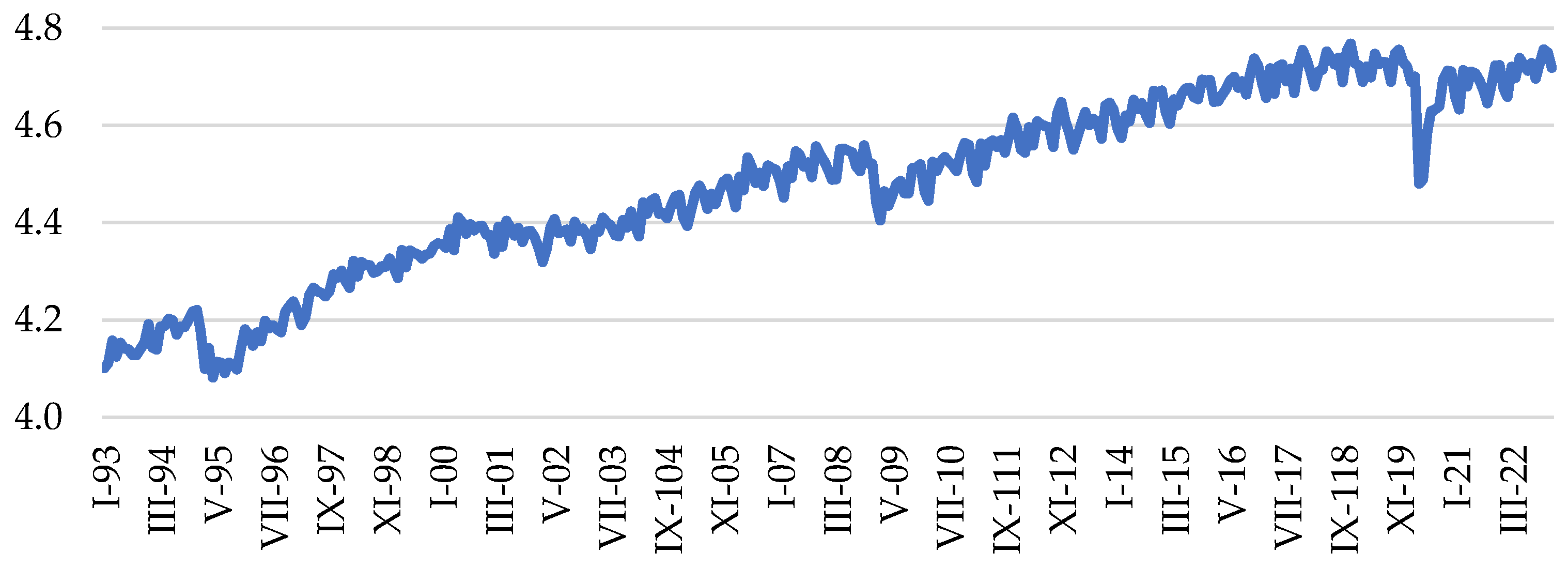
At the end of the entire analyzed period, in January 2023, the annual inflation rate reached 8.7%, the highest in the last 22 years. This was caused by an imbalance between supply and demand, primarily in the food and energy sectors. Inflationary pressures have been a consequence of the global pandemic, geopolitical tensions, and the ongoing Russia–Ukraine conflict. These factors led to increased pressures on agricultural and energy prices due to a slowdown in global economic activity and disruptions in supply chains. Mexico’s basic basket of goods of the past year had an increase of more than 10%, as well as services and goods influenced by external conditions with an increase of 6% (Banxico 2022). Figure 1 shows the transformation of the consumer price index into natural logarithms, aiming to decline potential heteroscedasticity, as well as to improve precision and ease comparison and understanding. This variable is shown at level I(0), and it will be analyzed later to obtain the stationary series (at level or first difference).
According to Elizondo (2012), the IGAE is a monthly economic variable and commonly used as an approximation of GDP, showing the temporal behavior of Mexico’s productive activity approximately 60 days after the end of the observed month. Its compilation is based on the national accounting method that follows the quarterly GDP, deciding the physical volume at a national level with primary, secondary, and tertiary activities, and with an approximation of 94.7% about the value added relative to the base year 2013 = 100 (INEGI 2013). Therefore, the IGAE can be a reliable benchmark for the monthly economic growth trend in Mexico. Figure 2 shows the economic activity index transformed into natural logarithms. This variable is shown at level I(0) and will be analyzed to obtain the stationary series (at level or first difference).
The use of natural logarithms in both indices, consumer prices and global economic activity, is useful to help stabilize variance and improve interpretability. Furthermore, this logarithmic transformation is useful when autoregressive models are used, facilitating the interpretation of the results as approximations in percentage changes.
As shown in Figure 2, in 1995, Mexico experienced a crisis triggered by a decrease in foreign capital inflows into the country, along with the devaluation of the Mexican peso and excessive borrowing due to a weak financial system (Banxico 2017). Over the past 14 years, two main periods of lower economic activity have been found. The first occurred at the end of February 2009 showing a low level of IGAE. This was due to Mexico’s commercial and economic dependence on the United States of America, as well as the weakening relationship with the financial sector. Globally, there was a significant contraction in manufacturing sectors, low stock market activity, and a decrease in energy, food, and commodity prices, reflecting a liquidity crisis in advanced economies. This affected emerging economies through reduced global demand, decreased trade volume, export restrictions, limited external financing, and an increase in unemployment levels (Banxico 2017).
All of the above events provide clarity on the need to consider that non-linearities in the relationship between inflation and growth can arise from a range of forces, including political uncertainty (Bloom 2009; Campello et al. 2022), domestic monetary policy (Hattori et al. 2016), and international monetary policy (Cortes et al. 2022). As a first experiment consider a simple reduced-form model as follows to shed some light on each channel:
l n I G A E t = β 0 + β 1 l n I N P C t + Γ i l n I N P C t × M a c r o F a c t o r s t + e t
where lnIGAEt represents the natural logarithm of the General Index of Economic Activity at time t; lnINPCt stands for the natural logarithm of the National Consumer Price Index at time t; MacroFactorst are various macroeconomic factors at time t, which can be represented by:
-
US Fed’s balance sheet (WALCL) as a proxy for the US unconventional monetary policy and its spillovers (Cortes et al. 2022), which considers changes in the size of the Federal Reserve’s balance sheet and liquidity provided can have significant implications for global financial markets, including Mexico (liquidity, interest rates, exchange rates, and investment flows);
-
Shadow rates (SR) (Wu and Xia 2016), as indicative of the monetary policy stance in economies practicing near-zero or negative interest rates. In this case, possible impacts are (1) monetary policy transmission (unconventional monetary policies of central banks), (2) risk appetite (lower shadow rates in major economies, increased risk appetite of investors flowing capitals into emerging markets), and (3) currency valuation (weakened currency in a major economy can make exports more competitive in emerging markets).
-
Global Policy Uncertainty Index (GPUI) (Davis 2016; Coronado et al. 2020) that measures the uncertainty related to economic policy globally, which can affect economic decision-making and outcomes, such as investment decisions (uncertain about future policies, more risk, and investment reduction), consumer behavior (economic growth reduction, inflation, job losses), trade flows (global economic conditions impact on exports and imports), and inflation expectations (adjustment of monetary policy in response to).
According to Table 1, β 1 suggests that there is a positive relationship between the consumer price index and economic activity, whereas the interaction terms of vector Γ i represent the combined effect of the consumer price index and the respective macroeconomic factor (i) on Mexican economic activity. The negative and significant coefficients for WALCL indicate less liquidity and increases in interest rates and exchange rates in Mexico. Shadow rates (tightening of monetary policy, making borrowing more expensive) imply that the impact of the consumer price index on economic activity is moderated or reduced as these macroeconomic factors increase. Notice that GPUI’s coefficient is close to zero but still negative, suggesting a negligible moderating effect from political instability, unpredictable economic policies, trade tensions, and financial market volatility. Therefore, the nature of these impacts depends on a variety of factors, including Banxico’s policy responses, global economic conditions, and the interaction of macroeconomic factors.

4. Methodology and Justification of the Nonlinear Autoregressive Distributed Lag (NARDL) Model

4.1. Limitations of Other Specifications

Before discussing the possibility of using a NARDL to identify the existence of a short- and long-term relationship (Pesaran and Shin 1995; Pesaran et al. 2001), it is worth reviewing some limitations of other common specifications. The Vector Autoregressive (VAR) model and the Vector Error Correction Model (VECM) introduced by Sargan (1964) and later used by Engle and Granger (1987), as a widespread testing technique, assume that variables have the same order of integration and stationarity. However, in many cases, not all variables have constant variance in the same order of integration; commonly at the first level or I(1), it can also be at I(0) but never equal to or greater than I(2). This also leads to addressing problems of autocorrelated errors when generating ARDL models. In this context, the limitations of symmetric long-term relationships will be quickly reviewed. Consider first a simple linear regression:
y t = α 0 + α 1 x t + e t ,
where α i represents the long-run parameters to be fitted, e t is with noise term, y t is the dependent or objective variable, which is l n I G A E t , and x t is the explicative or independent variable, which is l n I N P C t . Subsequently, an Error Correction Model (ECM) is considered as given by:
y t = β 0 + i = 1 p λ i y t i + i = 1 q δ i x t i + φ M C E t 1 + μ t ,
where y t i is the difference in l n I G A E t or monthly economic growth, x t i is the difference in l n I N P C t or monthly inflation, β 0 , λ i , and δ i are the short-term coefficients, M C E t 1 is the error correction term, and φ is the speed of adjustment (Majeed et al. 2020). Here,
M C E t 1 = u t 1 = y t 1 (   β 0 + φ 1 x t 1 ) .
In this way, Engle and Granger’s (1987) model requires two steps, which may complicate the estimation process. Another disadvantage is that it only requires variables of integration order I(1). Both disadvantages are not present in ARDL models, which only require one estimation step and consider variables of order I(1) or original level I(0). Therefore, the long-term estimation of the relationship between variables using the basic ARDL(p, q) model is as follows:
y t = β 0 + i = 1 p λ i y t i + i = 1 q δ i x t i + φ 1 y t 1 + φ 2 x t 1 + μ t .
The short-run terms ( i = 1 p λ i y t i + i = 1 q δ i x t i ) and long-run terms ( φ 1 y t 1 + φ 2 x t 1 ) are used to find the long-term relationship using the Bound Test (Pesaran and Shin 1995), with the null hypothesis stating that there is no long-term relationship. This is rejected when the F-Statistic value is greater than the Upper Critical Bound indicator. Considering the mentioned variables to be studied, y t i as the lagged target variable at time t (where i is the number of lags), x t i as the lagged explanatory independent variable at time t, refers to the difference operator, and μ t represents independent and identically distributed error terms with μ t   ~N(0,σ2). Meanwhile, the short-term coefficients are given by λ i and δ i , and the long-term coefficient is φ 1 useful for the validation of cointegration existence. The hypotheses to evaluate the presence of a long-term cointegration relationship among the proposed variables are as follows: H 0 = φ 1 = φ 2 = 0 y H 1 φ 1 φ 2 0 . That is, the null hypothesis tests for no cointegration versus the existence of a valid relationship between the l n I G A E t and the set of explanatory regressors. The optimal lags (ti) in the ARDL model can be determined by the Akaike Information Criterion (AIC) and the Schwartz Criterion (SC).
Finally, Allen and McAleer (2021) mentioned that ARDL models are widely used for estimating processes over time. However, as these models become more granular (high frequency), with dynamic specifications involving lags in I(0) and/or differences, it becomes challenging to obtain the necessary significances in the coefficients.

4.2. Setting Up the NARDL

Hossain et al. (2021) and Shin et al. (2014) argued that non-linearity is a widely observed situation in social sciences. An example is in developed and self-sufficient economies, a negative change in economic growth might be more surprising than a positive change. This situation is common as their economic activity is characterized by its resilience. Thus, positive or negative changes do not have the same impact capacity, making them asymmetrical or different (Bahmani-Oskooee et al. 2019), which is a category of non-linearity. Therefore, NARDL models can help in further understanding of asymmetries with the common assumption that the cointegration relationship involves a combination of stationary variables (Sargan 1964), and the first step is to analyze if this condition is accepted with the variables to use such as inflation and economic growth in Mexico. In general, the long-term relationship (cointegration) can be subject to asymmetries or non-linearities y = f ( x t + , x t ) .
As mentioned in the literature, the effect of basic product and service prices on economic activity growth could be asymmetric. Therefore, to analyze the asymmetric effect of the level of prices, l n I N P C t , on the economic activity growth, l n I G A E t , the NARDL model is chosen in the present investigation extending the linear approach of ARDL bounds testing.
After considering the asymmetry in (2), the following equation is obtained:
y t = α 0 + α 1 + x t + + α 2 x t + e t ,
where α 1 + and α 2 are long-term parameters to be estimated, while x t is a k × 1 vector of decomposed regressors as follows:
x t = x 0 + x t + + x t ,
where x t + and x t are partial sums in the processes of positive and negative changes in x t :
x t + = j = 1 t x j + ,
x t = j = 1 t x j .
Now, according to Pesaran and Shin (1995) and Pesaran et al. (2001), the NARDL model can be defined as follows:
y t = j = 1 p φ j y t j + j = 0 q ( θ j + x t j + + θ j x t j ) + ɛ t ,
y t = ρ y t 1 + θ 1 + x t 1 + + θ 2 x t 1 + j = 1 p 1 φ j y t j + j = 0 q 1 ( π j + x t j + + π j x t j + ɛ t ) .
Allen and McAleer (2021) explained Equation (11); p and q are the lag orders, θ j + and θ j are the asymmetric and autoregressive distributed lag parameters, and ε t represents independent and identically distributed error terms with zero mean and constant variance ( σ ε 2 ). In Equation (5), there is a potential hidden cointegration problem because it is not possible to give a correct interpretation of the estimated asymmetrical coefficient. To address this situation, a restriction is considered on the coefficients of Equation (6), such that α 1 + = θ 1 + / ρ and α 2 = θ 2 / ρ are the mentioned long-term increasing and decreasing impacts of x t on y t ; while j = 0 q π j + measures the influences of short-term increases of x t on y t . On the other hand, j = 0 q π j measures the influences of short-term decreases of x t on y t . Considering this, it follows
x t = j = 1 q 1 Λ j x t j + ν t ,
and
ɛ t = ω v t + e t = ω x t j = 1 q 1 Λ j x t j + e t ,
Thus, Equation (11) estimates the asymmetric impact of both short- and long-term effects of l n I N P C t ( x t ) on l n I G A E t ( y t ).
As mentioned before, the correction error ( Ω j ) is the speed of adjustment, in which a negative and meaningful relationship is expected with the dependent variable (Majeed et al. 2020). Therefore, the relationship is obtained from an Error Correction Model (ECM) within the NARDL as follows:
  y t = Ω j E C T t 1 + j = 1 p 1 φ j y t j + j = 0 q 1 ( τ j + x t j + + τ j x t j ) + e t ,
E C T t 1 = y t α 1 + x t + α 2 x t ,
where φ j is the short-term coefficient of the dependent variable, while τ j + and τ j represent the short-term asymmetry adjustment of the independent variable. On the other hand, Ω j refers to the coefficient of the nonlinear error correction term (NECT), which includes the long-term equilibrium considering asymmetry. Hence, the steps to be followed involve applying first-unit root tests to confirm whether the variables are integrated at order 0 or 1, or both. With this, using ordinary least squares, Equation (11) is enhanced to formulate the final form of the general NARDL model.

5. Empirical Results: Identification of Unit Root Test and the ARDL Model as First Step

This section is aimed at analyzing unit root tests of the variables under study and validating an ARDL model in order to comprehend the necessity of analyzing asymmetry and subsequently, implementing a NARDL model.

5.1. Unit Root Test

Table 2 presents the unit root tests for each variable, finding stationarity. For the identification of unit roots and integration of the variables, the Augmented Dickey–Fuller test (Dickey and Fuller 1981) and Phillips–Perron test (Phillips and Perron 1988) are applied. The stationarity of the variables is important to rule out the possibility of erroneous estimations.
The question of the long-term relationship will be evaluated using critical values determined for cases where the variables are stationary at level I(0) (levels) or I(1) (with first difference) but not greater than or equal to I(2). Therefore, for the variables of interest in this research, it was confirmed with unit root tests that the natural logarithm of the National Consumer Price Index at time t ( l n I N P C t ) is stationary at its normal level (without difference), while the natural logarithm of the Global Economic Activity Index at time t ( l n I G A E t ) is stationary in its first difference. The significance level of the probabilities of the variables shows that they are significant (less than 0.01), thus accepting the alternative hypothesis (existence of stationarity). Although the series are stationary at the level and first difference, the Kapetanios–Shin–Snell unit root test was conducted (Kapetanios et al. 2003). Therefore, the KSS test identifies that the statistic is greater than the levels of significance, leading to the conclusion that the series are stationary. With respect to the BDS test (Brock et al. 1996), the p-values of both series are lower than a given level of significance (such as 0.05 in this case). Hence, it is necessary to reject the null hypothesis, suggesting evidence of nonlinearity in the time series.

5.2. Validation and Application of the ARDL Model

For the application of the bounds test, the unrestricted error correction model is used (Seker et al. 2015). The formulation of the econometric model of Equation (5) provides an ARDL(12,9) model as follows (in long-run ARDL form):
y t = β 0 + i = 1 p λ i y t i + i = 1 q δ i x t i + φ 1 y t 1 + φ 2 x t 1 + μ t .
Considering l n I G A E t and l n I N P C t in long-run ARDL form, it follows that
l n I G A E t = β 0 + i = 1 p λ i l n I G A E t i + i = 1 q δ i l n I N P C t i + φ 1 l n I G A E t 1 + φ 2 l n I N P C t 1 + μ t .
Therefore, the Error Correction Model of the ARDL model is
l n I G A E t = β 0 + i = 1 p λ i l n I G A E t i + i = 1 q δ i l n I N P C t i + φ M C E t 1 + μ t .
The econometric breakdown of the ARDL for Error Correction Model satisfies the following:
l n I G A E t = 0.37 l n I G A E t 1 0.35 l n I G A E t 2 0.27 l n I G A E t 3 0.32 l n I G A E t 4 + 0.01 l n I G A E t 5 * 0.12 l n I G A E t 6 0.04 l n I G A E t 7 * 0.18 l n I G A E t 8 0.17 l n I G A E t 9 0.29 l n I G A E t 10 0.28 l n I G A E t 11 0.36 l n I N P C t * 0.69 l n I N P C t 1 + 0.43 l n I N P C t 2 * 0.84 l n I N P C t 3 + 1.69 l l n I N P C t 4 1.23 l n I N P C t 5 0.07 l n I N P C t 6 * 0.46 l n I N P C t 7 * + 1.23 l n I N P C t 8 0.05 C o i n t E q t 1 .
In this case (*) represents variables outside significance level 5% and 10%, and Table 3 illustrates the p-value or Prob. according to Eviews 12. In the next section, with the results of the stationarity analysis and the application of the Ramsey test, it will be possible to identify the existence of an asymmetric relationship in the short and long term for l n I G A E t and l n I N P C t .

6. Empirical Results of the Asymmetric Relationship and Identification of the Optimal NARDL Model

Arize et al. (2017) suggested that the variables with a varied order of integration do not show a long-term relationship in the traditional sense, so an econometric analysis of the long-term relationship should be varied. In this sense, hidden cointegration between variables, also called long-term nonlinear association, cannot be assessed using the conventional ARDL approach. In this sense, considering the specification proposed (Brock et al. 1996), a Regression Equation Specification Error Test (RESET) will be conducted since there are specification errors due to lack of information indicating the necessary reactions to show the long-term relationship, see Table 4.
According to Table 4, it was found that the probability of the t-statistic and the F-statistic is less than 5%, so the null hypothesis is rejected, suggesting the existence of asymmetry or non-linearity between the price level and global economic activity in Mexico.

6.1. Optimal Lags for NARDL

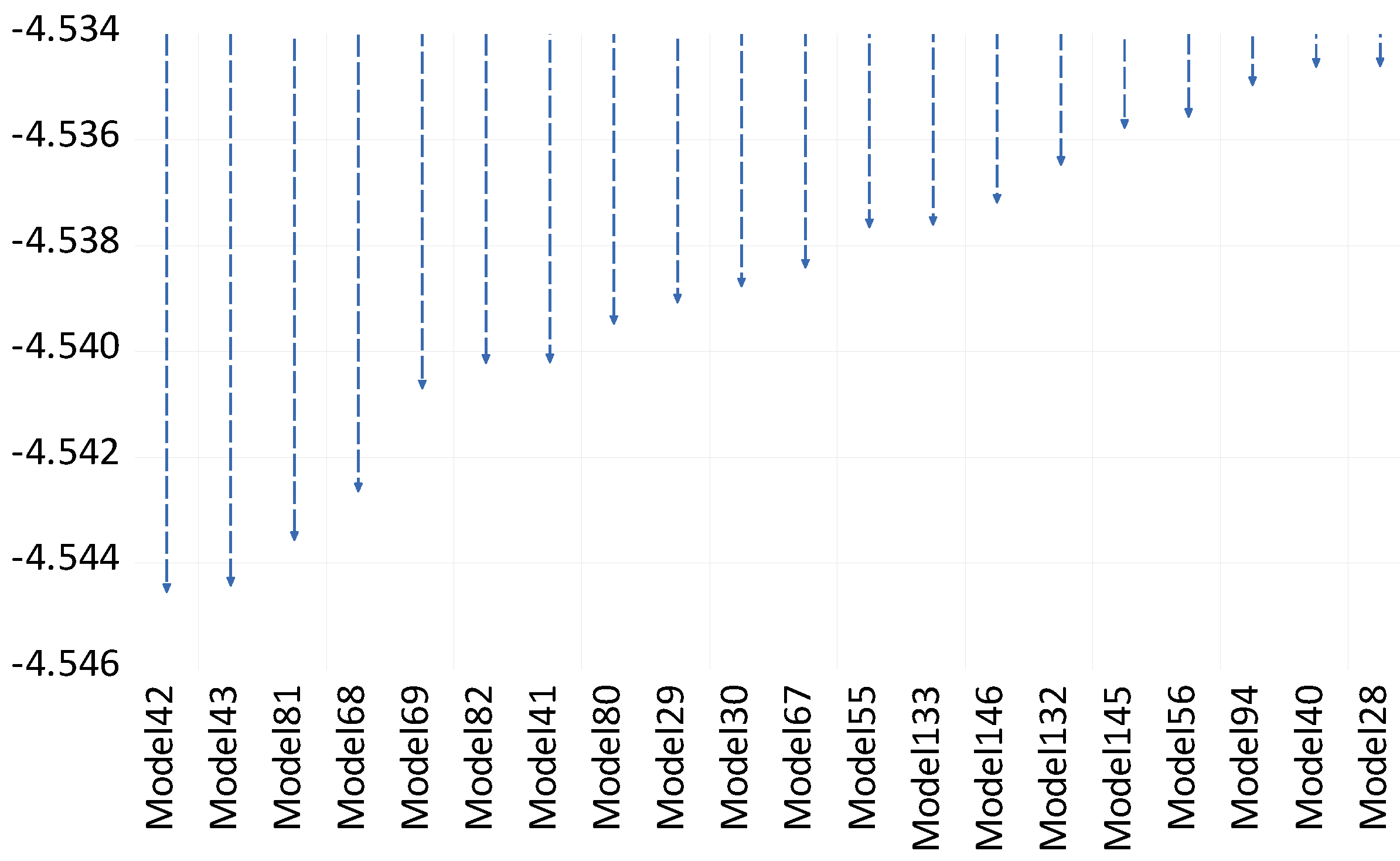
Once the stationarity has been stated and the asymmetry of the studied variables has been shown, the next step is to select the parsimony of the NARDL model by the optimal lag and thereby estimate the cointegration relationship. Figure 3 shows the optimal selection of lags and the estimation of the cointegration relationship between them using the specific optimal lag Akaike Information Criterion (AIC).
Among the various criteria available, the Akaike Information Criterion (AIC) holds merit over others in certain scenarios due to its theoretical foundation and practical benefits. When dealing with a monthly NARDL model, the AIC might be preferred over other criteria. The AIC considers both the goodness of fit and the complexity of the model and helps to prevent over-fitting. In a monthly NARDL model, it is possible to have different lag lengths for different variables. It is also important to have a balance between capturing the dynamics of the process and avoiding overly complex models. Also, the AIC aims to select a model that not only fits the observed data well but also generalizes well to new data. Moreover, the AIC encourages parsimony, meaning that it is preferred to have models with fewer parameters. This can lead to more interpretable models that are easier to explain. In the context of a monthly NARDL model, various lag lengths can be considered. With no prescribed distribution, the AIC does not rely on distributional assumptions about the data, making it applicable across a wide range of models, including nonlinear models like NARDL. Finally, the choice of lag length criteria can also depend on the specific characteristics of data, the underlying economic theory, and the goals of the analysis.

6.2. Estimation and Optimization of Asymmetry

Considering the Granger causality test (Granger 1969), the objective is to figure out if the lagged values of a variable are correlated with the current values of another variable. Table 5 presents a unidirectional relationship from the independent variable l n I N P C t with two lags and a confidence level of 95% toward the dependent variable l n I G A E t . This test is based on the Vector Autoregressive Model (VAR). Another option to prove causality was that of Toda and Yamamoto (1995), which shows a causality from l n I N P C t toward l n I G A E t . The probability values, in Table 4, show that there is not enough evidence to reject the alternative hypothesis for the independent variable, thus l n I N P C t Granger causes l n I G A E t .
Now the NARDL model developed by Shin et al. (2014) was considered to cover the deficiencies of the classical ARDL by including long-term non-linear associations. The econometric Equation (11) is used to conduct the optimization of the data, as shown in Table 5.
The vector fitted is corroborated with a diagnostic test with an ordinary R2 of 98.36%, showing that the goodness of fit is high (see Table 5) (Adeleye et al. 2023; Wang et al. 2020). The asymmetric long-run coefficients are also given in Table 5 and reveal the asymmetric cointegration equation in which for each unit of change in the level of the price index, whether positive or negative, the monthly economic activity has an impact of 0.138% and 2.12%, respectively, with significant levels (p-values less than 0.01 or 1%). With respect to the Bayer and Hanck test cointegration (Bayer and Hanck 2013), it shows test statistic values of Engle and Granger (1987), EG-J or Johansen (1991), Boswijk (1995), and EG-J-BG-BO or Banerjee (1998), with 23.84 and 55.14 are higher than 5% of critical value, 11.23 and 21.93, respectively. So, the null hypothesis of no cointegration was rejected. This supports the NARDL cointegration test, which also revealed the presence of a long-run relationship with two variables.
Taking into account the coefficients obtained α 1 + = 0.13 and α 2 = 2.1 , and considering the coefficients of Equation (6) with their values shown in Table 5, the impacts are identified with increases and reductions in the long term of x t ( l n I N P C t ) on y t ( l n I G A E t ). This is because the results reveal that the consumer price index has an asymmetric impact on the levels of monthly economic activity, in addition to greater actions to reduce the price index  l n I N P C t , which causes costs to the economic activity, while the increase in prices l n I N P C t +  leads to a slight increase in economic activity. In this sense, Atil et al. (2014) argued that a factor of non-linear asymmetric behavior of the vectors or macroeconomic variables occurs in times of economic crisis, as is the case for Mexico as a result of the global pandemic COVID-19 2020–2022.
The existence of a relationship according to Equation (11) is proven through the F-Bounds test statistic to assess the importance of the lagged levels of the variables in an ECM and confirm the long-term significance (Narayan 2004). Hence, as shown in Table 5, after using an Ordinary Least Squares (OLS) regression, the results for the long term are that the coefficient in the lagged error correction term is significant (0.0000) with the expected negative sign, which confirms the result of the limits test for cointegration. Therefore, the CointEq(−1) shows a value of −0.1138, which implies the slow rate of adjustment to equilibrium of 11.38% after a shock. Hence, the causality runs interactively through the error correction term.
In the same Table 5, the asymmetric ECM satisfies the rule with a NARDL model (Shin et al. 2014), since the value of the F-Bound statistic (4.42) is greater than the highest critical value of the selected significance levels of I(1), which leads to the acceptance of the alternative hypothesis regarding the existence of a non-linear cointegration relationship between the level of consumer prices ( l n I N P C t ) and the variation in global economic activity ( l n I G A E t i ).

6.3. Long-Run Form (LRF) Asymmetric Test and Wald Test Validation

An important result of the NARDL, stated in Table 5, is the long-run form (LRF). Therefore, it is needed to confirm the optimal long-term cointegration behavior with the stepwise regression validation by selecting the unidirectional Fowards method, in addition to the p-value 0.05, which shows the nonlinear parsimony (asymmetry) of the ECM, obtaining the following results as shown in Table 6.
The long-term variables are above the dotted horizontal line in Table 6, while the short-term ones are below it. Note all insignificant short-term variables are excluded, although all long-term ones are kept, whether they are or not significant. Different lags in Table 6 confirm that they are not always significant in NARDL models, but that they can be preserved as having larger lags significant. These kinds of models are complex by nature due to the inclusion of lagged variables and nonlinear terms, but stepwise regression helps in constructing a parsimonious model by selecting only those variables that contribute significantly to explaining the variation in the dependent variable. With the results of the estimation of errors in Table 6, the Wald test was applied to justify the asymmetry of the cointegration in the long-term coefficients (−c(3)/c(2) = −c(4)/c(2)) and short term (c(5) to c(13)), see Table 7.
According to the stepwise regression, there is evidence of asymmetry in the relationship of l n I G A E t and l n I N P C t (Kassi et al. 2019; Sowah et al. 2023; Allen and McAleer 2021). Considering the results of Table 7 with a Chi-square p-value less than 0.05, the existence of asymmetry in the period is confirmed.
Also note that the results shown in Table 6 also indicate that when an upward movement of positive inflation Δ( l n I N P C + ) is statistically significant, it has a negative impact on the increase in the global indicator of economic activity in the short term (Okun 1971; Friedman 1977; Phelps 1969). This impact is greater on the growth of the global indicator of economic activity when there are actions that cause a decrease in inflation Δ( l n I N P C ). It is worth mentioning that the consumer price index decreases, without good monetary policy control, which is also undesirable because consumers delay purchases, and this translates into less economic activity, less income generated by producers, and less economic growth (Siaens 1969). While, in the long term, the increase in the consumer price index has a slight and better effect on economic activity, supporting the ideas mentioned by Azariadis and Smith (1996) with the Mundell–Tobin effects.
In summary and confirming various investigations (Atkeson and Kehoe 2004; Borio and Filardo 2004; Bordo and Redish 2004), the benefits could be positive in the global economic activity if the monetary policy of Banxico continues in the direction of controlling the level of the consumer prices index through applicable actions, such is the case of the reference interest rate, but taking care of the impact on economic activity as a result of the increase in demand.
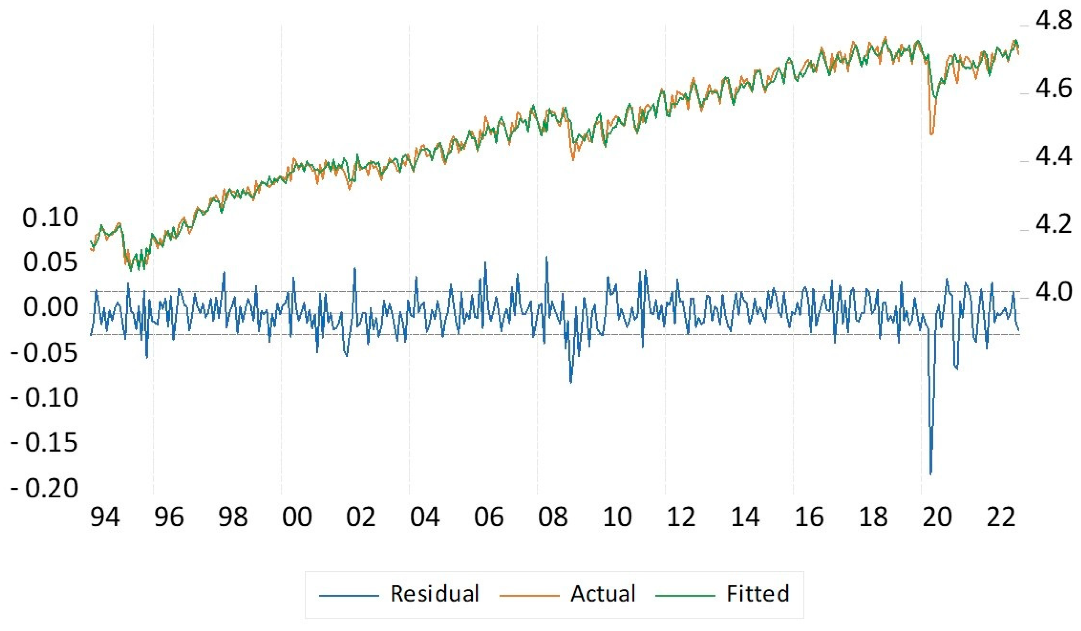
In the research of Tinoco-Zermeño et al. (2014), although the necessary tests were carried out to validate that there is no serial autocorrelation (Lagrange Multiplier test) nor heteroskedasticity by Breusch–Pagan–Godfrey test, the information in Table 5 suggests the presence of autocorrelation and homoscedasticity with significant levels at 5%, which is related to the nonlinearity of the variables used in the present research. The absence of normal residuals could also lead to the application of quantile models in future studies (Brooks 2019; Cho et al. 2015). In this case, the results obtained with stepwise regression (Chen et al. 2021; Gao et al. 2022) are shown in Table 6, providing a Durbin Watson value of 1.80, which does not reflect a concern of autocorrelation. In this way, validating that both behaviors are similar between the long- and short-term coefficients obtained with the NARDL Long-Run Form model and optimization through stepwise regression. Figure 4 shows the simulation of the behavior of l n I G A E t in the function of l n I N P C t using the NARDL (12,9,10) model.
With the behavior shown in Figure 4, the vector fitted is corroborated with good behavior versus the current one.

6.4. Asymmetric Dynamic Multipliers

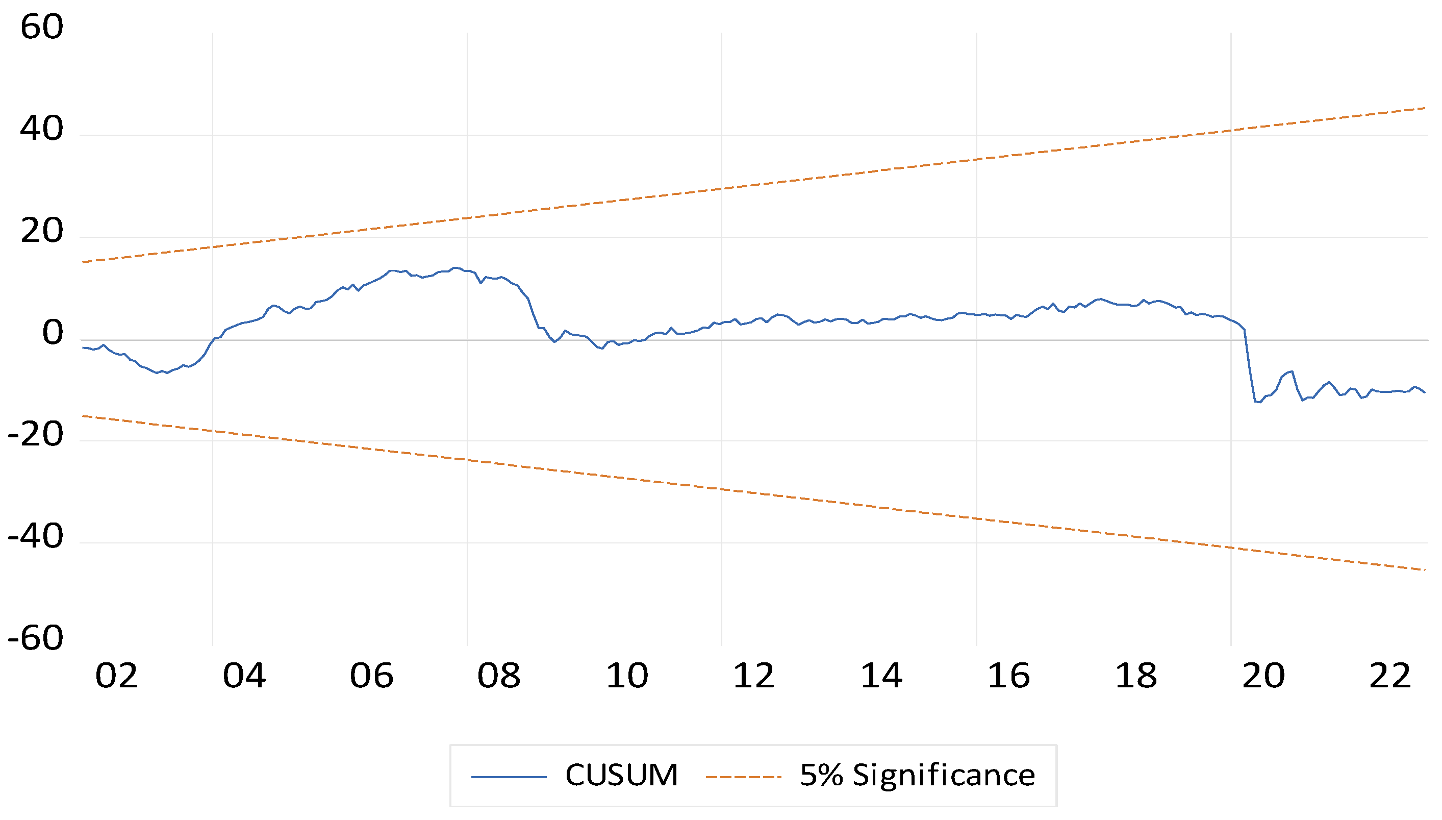
In order to explore whether the estimated coefficients are stable in the short and long term (Pan et al. 2022; Das et al. 2023), the Cumulative Sum of Error Forecast (CUSUM) test is applied to verify stability (Pesaran et al. 2001). The results are shown in Figure 5 with a 5% confidence band, and all the values in the sample are identified even considering the subprime crisis of 2009 and the effects of the COVID-19 health emergency between the years 2020 and 2022. Figure 5 indicates that CUSUM values are within the band and implies that the optimal NARDL (12,9,10) model adequately captures the nonlinear effects of consumer price levels on the indicator of economic activity in Mexico.
However, in Figure 5, as of 2020, a departure from the average is noted due to the international situation, as well as the effects of internal economic activity, which implies that the effects of economic instability will continue to be present in the short term for the Mexican case as shown by the Breusch–Pagan–Godfrey test displayed in Table 5.
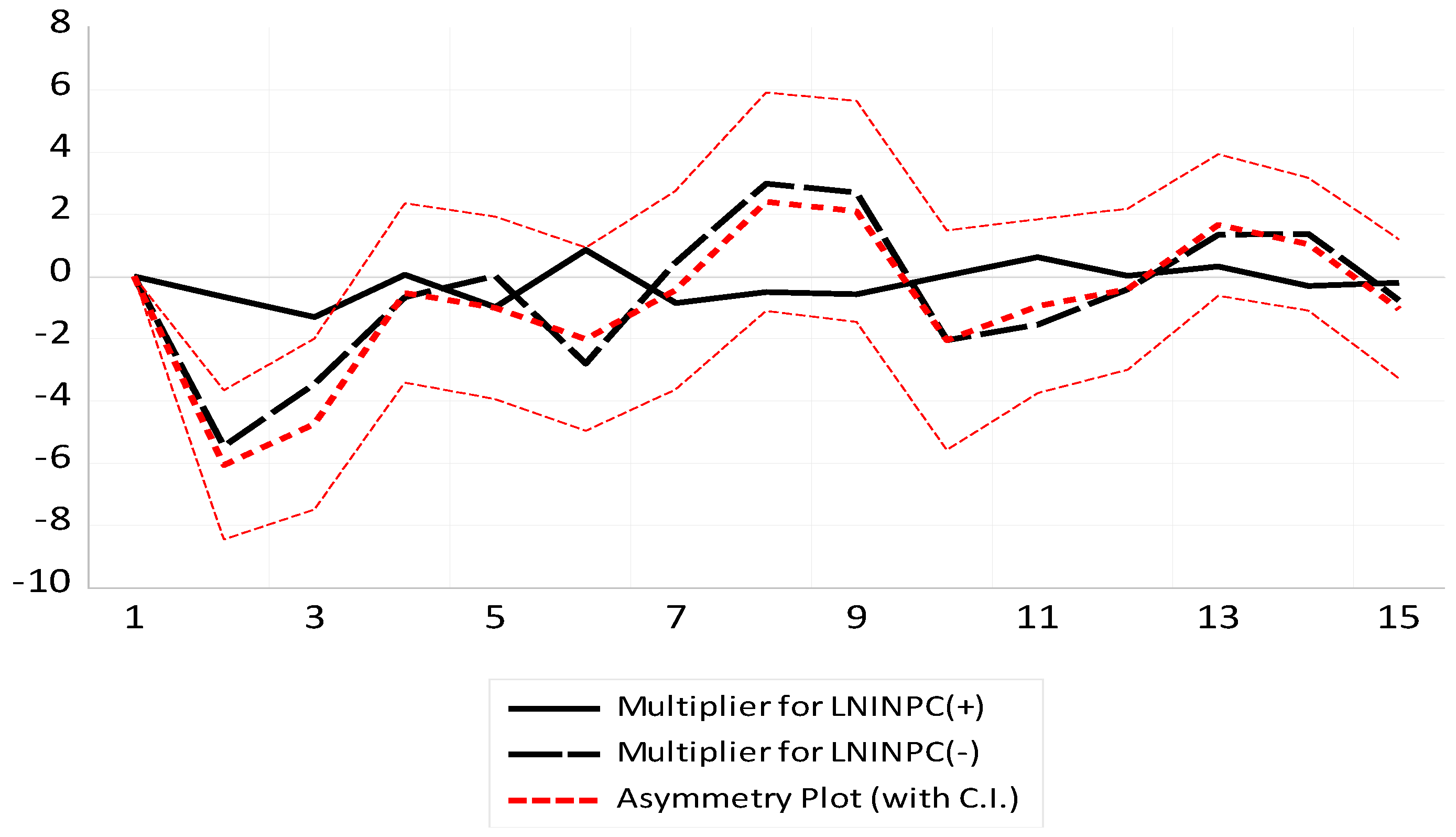
On the other hand, to explain the movement of economic activity and its quick response to cyclic increases and decreases in consumer price levels, we employed the modeling proposal from Shin et al. (2014), and after a shock in the consumer prices index, there are both positive and negative effects on economic activity, with dynamic adjustments over time.
As shown in Figure 6, with the dynamic multipliers for Mexico, greater dynamism in the business cycle occurs when there is a contractionary shock in consumer prices (multiplier for l n I N P C ) . This arises through measures aimed at controlling and reducing prices, which is a good message for agents. Additionally, the equilibrium error tends to correct itself over time.

7. Discussion of the Empirical Results

Many empirical works that have been conducted conclude that there are both internal and external variables that can influence economic growth measured by quarterly (Cerezo-García et al. 2019) or annual GDP (Tinoco-Zermeño et al. 2014). However, this paper raises the possibility of showing the dynamism of economic activity in a monthly period to examine the effects of asymmetric movements of the National Consumer Price Index in Mexico. First, the Mexican results of the unit root test are related to Hossain et al. (2021) and Tinoco-Zermeño et al. (2014), where the condition is accepted with levels I(0) or first differences I(1).
Therefore, the NARDL (12,9,10) model conducted in this research is useful for verifying the existence of a monthly cointegration relationship in Mexico between global economic activity and the level of consumer prices. Specifically, the NARDL model covers the ARDL deficiency helping to show the analysis of long-term nonlinear associations (Tinoco-Zermeño et al. 2014; Olugbenga and Dada 2020; Karahan and Çolak 2020; Cerezo- García et al. 2019). The NARDL model was used considering the results in Table 2 for stationarity analysis, order of integration, and non-linearity, where it was identified that lnIGAE is stationary at level I(0) and lnINPC at first level I(1), which meets the requirement for possible consideration in NARDL models. The second requirement was with the results of the asymmetry analysis from the Ramsey test, which indicates a more appropriate application of the NARLD models. The verifications of the econometric tests not only confirm the relationship of the variables with the proposed model but also show an area of structural instability with respect to the average in the period from 2008 (Cerezo-García et al. 2019) and 2019 to 2023, as can be seen in the CUSUM test.
In relation to the Phillips Curve, there are many analyses not only in emerging markets but also in developed economies (Hazell et al. 2022). The results of this research provide empirical support to this concept, at least in the context of the relationship between inflation and economic activity. In short term, higher positive inflation Δ( l n I N P C + ) is correlated with a decrease in economic growth ( l n I G A E t ), and higher negative inflation Δ( l n I N P C ) is correlated with an increase in economic growth ( l n I G A E t ). It is important to note, however, that these results do not directly measure unemployment, which is the other key variable in the Phillips Curve. Additionally, the long-term relationship is captured with a lag in this context, suggesting that past inflation influences current economic activity, which is a dynamic aspect worth considering in policy analysis and economic forecasting.

7.1. Short-Term Implications

Regarding costs for decision makers and policymakers, with the results in Table 5 and Table 6, there is a considerable increase in the economic activity of Mexico Δ( l n I G A E t ) when opting for contractive monetary measures to reduce consumer price levels Δ( l n I N P C ). The present research is significant in the same direction as observed in studies for Bangladesh (Hossain et al. 2021) and Turkey (Karahan and Çolak 2020).
On the other hand, when there is no intervention of monetary policy and prices rise Δ( l n I N P C + ), the economic growth is affected negatively as observed in studies by Cerezo-García (2019), while Hossain et al. (2021) and Karahan and Çolak (2020) present contrasting perspectives.

7.2. Long-Term Implications

Notable results in Table 5 and Table 6 show that the growth of the economic activity index Δ( l n I G A E t ) would be insignificant if there is an increase in consumer price levels l n I N P C 1 + . While if there were greater control of prices or a decrease in the level of the consumer prices index l n I N P C 1 , then the economic activity decreases.
Under the above context, the results obtained coincide with that of Okun (1971), Friedman (1977), and Phelps (1969), an increase in prices will reduce economic growth; while Azariadis and Smith (1996), Atkeson and Kehoe (2004), Borio and Filardo (2004), Bordo and Redish (2004) obtain an inverse relationship between inflation and economic growth.
The positive and negative shocks in consumer prices can be caused by multiplier effects (Olugbenga and Dada 2020; Alharbi 2022), mainly when there is a downward movement, there is a greater impact on the global economic activity. This particularly illustrates the asymmetric trends of the l n I N P C t multiplier, incorporating significant shocks both positive and negative. In the case of l n I N P C t + ,  the effect is positive, but the negative impact of l n I N P C t is higher on Δ( l n I G A E t ) as identified by Cerezo-García et al. (2019) and Karahan and Çolak (2020). However, in studies on Bangladesh, the consumer price shocks are identified to have no contrary effects, as both are positive at the same level (Hossain et al. 2021), while in studies on Turkey, the effects on economic growth are negative in both directions of the price shock (Karahan and Çolak 2020).

8. Conclusions

The trajectory of inflation in recent periods in Mexico has been affected by international events, so their accumulated effects have risen to significant levels of inflation. These levels above the objective set by Banxico have brought the effectiveness of monetary policy into question and that is why it has managed it with the determination to raise the interest rate in recent times and has been expectant about the variables that may influence it.
Under the proposed NARDL (12,9,10) model, the nature of the asymmetry and cointegration connection between the variables was demonstrated both in the long and short term. Over the last almost 30 years, the results effectively show that there is evidence of nonlinearity in different negative and positive effects on monthly economic growth in both the short and long term for the Mexican economy. In general, it was found that in the short term, a decrease in consumer prices is beneficial for economic growth in Mexico with available monthly information (Okun 1971; Friedman 1977; Phelps 1969), while in the long term, there is less impact on economic activity when there is more control with monetary policy actions (Azariadis and Smith 1996). Therefore, monetary policy strategies are needed to optimally address these events and give a strategic boost to global economic activity in Mexico, considering the short- and long-term costs–benefits found in this research using the NARDL model.
As mentioned before, for policymakers, understanding threshold effects and nonlinearity becomes crucial to reformulating effective economic policies. Considering the importance of high-frequency data in this kind of models allows interactions between these variables at a finer temporal resolution considering the fast-moving economic environments (Sánchez-Vargas and López-Herrera 2020; Saucedo and Gonzalez 2021). Keeping stable inflation rates below the identified threshold can promote sustainable economic growth by avoiding the possible negative impacts that high inflation can have on the economy. High inflation rates can erode purchasing power, create uncertainty in economic planning, and discourage long-term investment.
For academic researchers, economic agents, and policymakers, understanding the nonlinear relationship between inflation and economic growth opens up new avenues for future investigation and analysis. This encourages the exploration of additional factors that may influence the relationship and identification of other threshold levels. Additionally, these findings underscore the importance of using more sophisticated and appropriate models, such as NARDL models. This modeling can better capture the complexities of real-world economic dynamics and produce more reliable policy recommendations. Recognition of non-linearity and threshold effects allows for more targeted and effective policy interventions to ensure sustainable economic growth while mitigating the risks associated with high inflation rates.
This paper urges future research to verify the degree of impact of the acceleration of prices and the slow growth of economic activity in Mexico, as well as the consideration of fiscal policy for the strengthening of the tax structure, which could give greater adjustment and inflationary containment, both on the supply and demand sides. This could be achieved by adopting better strategies to subsidize some foods, containing price increases with the producing sector and supply chains, as well as agricultural and industrial policies to reduce external dependence.

Author Contributions

Conceptualization J.C.T.-G. and M.D.L.S.-R.; methodology and software, J.C.T.-G.; validation, J.C.T.-G., R.V.-R. and F.V.-M.; formal analysis and investigation, J.C.T.-G. and R.V.-R.; data preparation, M.D.L.S.-R. and F.V.-M.; writing—original draft preparation, J.C.T.-G.; writing—review and editing, R.V.-R., J.C.T.-G., M.D.L.S.-R. and F.V.-M. All authors have read and agreed to the published version of the manuscript.

Funding

This research was funded by Instituto Politécnico Nacional, grant number SIP20231902, and registered by Secretaría de Investigación y Posgrado, Instituto Politécnico Nacional.

Informed Consent Statement

Not applicable.

Data Availability Statement

The paper uses publicly available data. Sources and data are defined in Section 3.

Conflicts of Interest

The authors declare no conflicts of interest. The funders had no role in the design of the study; in the collection, analysis, and interpretation of data; in the writing of the manuscript; and in the decision to publish the results.

References

  1. Adeleye, Bosede Ngozi, Sodiq Arogundade, and Biyase Mduduzi. 2023. Empirical Analysis of Inclusive Growth, Information and Communication Technology Adoption, and Institutional Quality. Economies 11: 124. [Google Scholar] [CrossRef]
  2. Al Khatib, Abdullah Mohammad Ghazi. 2023. The complexity of financial development and economic growth nexus in Syria: A nonlinear modelling approach with artificial neural networks and NARDL model. Heliyon 9: e20265. [Google Scholar] [CrossRef] [PubMed]
  3. Alharbi, Farea Mohammed. 2022. How Do the Remittance Outflows React to Economic Development in Saudi Arabia? Evidence from NARDL. Economies 10: 105. [Google Scholar] [CrossRef]
  4. Allen, David, and Michael McAleer. 2021. A Nonlinear Autoregressive Distributed Lag (NARDL) Analysis of the FTSE and S&P500 Indexes. Risks 9: 195. [Google Scholar] [CrossRef]
  5. Anda, Milin Ioana, Bușan Gabriela, Ecobici Nicolae, and Abdul Rehman. 2023. Economic Growth Drivers in Romania: Evidence from a NARDL Analysis. Sustainability 15: 5916. [Google Scholar] [CrossRef]
  6. Arize, Augustine C., John Malindretos, and Emmanuel U. Igwe. 2017. Do Exchange Rate Changes Improve the Trade Balance: An Asymmetric Nonlinear Cointegration Approach. International Review of Economics & Finance 49: 313–26. [Google Scholar] [CrossRef]
  7. Atil, Ahmed, Amine Lahiani, and Duc Khuong Nguyen. 2014. Asymmetric and Nonlinear Pass-through of Crude Oil Prices to Gasoline and Natural Gas Prices. Energy Policy 65: 567–73. [Google Scholar] [CrossRef]
  8. Atkeson, Andrew, and Patrick J. Kehoe. 2004. Deflation and Depression: Is There an Empirical Link? American Economic Review 94: 99–103. [Google Scholar] [CrossRef]
  9. Azariadis, Costas, and Bruce D. Smith. 1996. Private Information, Money, and Growth: Indeterminacy, Fluctuations, and the Mundell-Tobin Effect. Journal of Economic Growth 1: 309–32. [Google Scholar] [CrossRef]
  10. Bahmani-Oskooee, Mohsen, Dan Xi, and Sahar Bahmani. 2019. More Evidence on the Asymmetric Effects of Exchange Rate Changes on the Demand for Money: Evidence from Asian. Applied Economics Letters 26: 485–95. [Google Scholar] [CrossRef]
  11. Bailey, Warren, Kalok Chan, and Y. Peter Chung. 2000. Depositary receipts, country funds, and the peso crash: The intraday evidence. The Journal of Finance 55: 2693–717. [Google Scholar] [CrossRef]
  12. Bailey, Warren, and Peter Chung. 1995. Exchange rate fluctuations, political risk, and stock returns: Some evidence from an emerging market. Journal of Financial and Quantitative Analysis 30: 541–61. [Google Scholar] [CrossRef]
  13. Banerjee, Jyotirmoy. 1998. United Germany: Quo Vadis? Jadavpur Journal of International Relations 4: 1–12. [Google Scholar] [CrossRef]
  14. Banxico. 2009. Inflation Report January—March 2009 Resume. Banco de México. CDMX, Mexico. April 28. Available online: https://www.banxico.org.mx/publicaciones-y-prensa/informes-trimestrales/%7BE5FA3814-DF51-6A97-1B9E-AEF929F93A5E%7D.pdf (accessed on 1 September 2023).
  15. Banxico. 2017. Executive Summary, Quarterly Report October—December 2017. Banco de México. CDMX, Mexico. December 31. Available online: https://www.banxico.org.mx/publicaciones-y-prensa/informes-trimestrales/%7B263682EB-EEC3-BCD1-BF5E-A595871E8EB8%7D.pdf (accessed on 31 December 2023).
  16. Banxico. 2022. Press Release. Monetary Policy Announcement. Banco de México. CDMX, Mexico. September 29. Available online: https://www.banxico.org.mx/publicaciones-y-prensa/anuncios-de-las-decisiones-de-politica-monetaria/%7BE6A0E26E-D9C0-97D7-64B7-7F2BF274178E%7D.pdf (accessed on 1 December 2023).
  17. Barro, Robert. 1995. Inflation and Economic Growth. Cambridge: National Bureau of Economic Research. [Google Scholar] [CrossRef]
  18. Bayer, Christian, and Christoph Hanck. 2013. Combining Non-Cointegration Tests. Journal of Time Series Analysis 34: 83–95. [Google Scholar] [CrossRef]
  19. Bloom, Nicholas. 2009. The Impact of Uncertainty Shocks. Econometrica 77: 623–85. [Google Scholar] [CrossRef]
  20. Bordo, Michael D., and Angela Redish. 2004. Is Deflation Depressing? Evidence From the Classical Gold Standard. In Deflation. Edited by Burdekin Richard and Siklos Pierre. Cambridge: Cambridge University Press, pp. 191–217. [Google Scholar] [CrossRef]
  21. Borio, Claudio, and Andrew Filardo. 2004. Back to the Future? Assessing the Deflation Record. No. 152. Basel: Bank for International Settlements. [Google Scholar] [CrossRef]
  22. Boswijk, H. Peter. 1995. Efficient Inference on Cointegration Parameters in Structural Error Correction Models. Journal of Econometrics 69: 133–58. [Google Scholar] [CrossRef]
  23. Brock, William, Davis Dechert, and José Sheinkman. 1996. A Test of Independence Based on the Correlation Dimension. Econometric Reviews 15: 197–235. Available online: https://scholar.google.com/scholar_lookup?journal=Econom.+Rev.&title=A+test+for+independence+based+on+the+correlation+dimension&author=W.A.+Brock&author=J.A.+Scheinkman&author=W.D.+Dechert&author=B.+LeBaron&volume=15&publication_year=1996&pages=197-235&doi=10.1080/07474939608800353& (accessed on 1 September 2023). [CrossRef]
  24. Brooks, Chris. 2019. Introductory Econometrics for Finance. Cambridge: Cambridge University Press. [Google Scholar] [CrossRef]
  25. Campello, Murillo, Gustavo Cortes, Fabrício d’Almeida, and Guarav Kankanhalli. 2022. Exporting Uncertainty: The Impact of Brexit on Corporate America. Journal of Financial and Quantitative Analysis 57: 3178–222. [Google Scholar] [CrossRef]
  26. Cerezo-García, Verónica, Teresa S. López-González, and Francisco López-Herrera. 2019. Crecimiento Económico e Inflación En México, 1993–2018: ¿Una Relación Lineal o No Lineal? Investigación Económica 79: 83. [Google Scholar] [CrossRef]
  27. Chang, Chiu-Lan, and Ming Fang. 2023. Impact of a Sharing Economy and Green Energy on Achieving Sustainable Economic Development: Evidence from a Novel NARDL Model. Journal of Innovation & Knowledge 8: 100297. [Google Scholar] [CrossRef]
  28. Chen, Hao, Duncan O. Hongo, Max William Ssali, Maurice Simiyu Nyaranga, and Consolata Wairimu Nderitu. 2020. The Asymmetric Influence of Financial Development on Economic Growth in Kenya: Evidence From NARDL. SAGE Open 10: 2158244019894071. [Google Scholar] [CrossRef]
  29. Chen, Tinggui, Lijuan Peng, Jianjun Yang, and Guodong Cong. 2021. Analysis of User Needs on Downloading Behavior of English Vocabulary APPs Based on Data Mining for Online Comments. Mathematics 9: 1341. [Google Scholar] [CrossRef]
  30. Cho, Jin Seo, Tae-hwan Kim, and Yongcheol Shin. 2015. Quantile Cointegration in the Autoregressive Distributed-Lag Modeling Framework. Journal of Econometrics 188: 281–300. [Google Scholar] [CrossRef]
  31. Coronado, Semei, José N. Martínez, and Francisco Venegas-Martínez. 2020. Spillover Effects of the US Economic Policy Uncertainty in Latin America. Estudios de Economía 47: 273–93. Available online: https://estudiosdeeconomia.uchile.cl/index.php/EDE/article/view/59173 (accessed on 1 September 2023). [CrossRef]
  32. Cortes, Gustavo S., George P. Gao, Felipe B. G. Silva, and Zhaogang Song. 2022. Unconventional Monetary Policy and Disaster Risk: Evidence from the Subprime and COVID-19 Crises. Journal of International Money and Finance 122: 102543. [Google Scholar] [CrossRef]
  33. Das, Anupam, Leanora Brown, and Adian McFarlane. 2023. Asymmetric Effects of Financial Development on CO2 Emissions in Bangladesh. Journal of Risk and Financial Management 16: 269. [Google Scholar] [CrossRef]
  34. Davis, Steven J. 2016. An Index of Global Economic Policy Uncertainty. Macroeconomic Review. Cambridge: National Bureau of Economic Research. [Google Scholar] [CrossRef]
  35. Dickey, David A., and Wayne A. Fuller. 1981. Likelihood Ratio Statistics for Autoregressive Time Series with a Unit Root. Econometrica 49: 1057. [Google Scholar] [CrossRef]
  36. Ekpeyong, Paul. 2023. Econometric Analysis of the Impact of Inflation, Unemployment, and Economic Growth on Poverty Reduction: A Novel Application of Asymmetric Technique. Munich Personal RePEc Archive. Available online: https://mpra.ub.uni-muenchen.de/117762/1/INFLATION%2C%20UNEMPLOYMENT%2C%20ECONOMIC%20GROWTH%20ON%20POVERTY.pdf (accessed on 31 December 2023).
  37. Elizondo, Rocio. 2012. Estimaciones Del PIB Mensual Basadas En El IGAE. 2012–11. CDMX, Mexico. Available online: https://www.banxico.org.mx/publicaciones-y-prensa/documentos-de-investigacion-del-banco-de-mexico/%7BB583DA23-0F6A-2F56-3B50-F575F405EEB1%7D.pdf (accessed on 1 September 2023).
  38. Engle, Robert F., and C. W. J. Granger. 1987. Co-Integration and Error Correction: Representation, Estimation, and Testing. Econometrica 55: 251. [Google Scholar] [CrossRef]
  39. Fischer, Stanley. 1993. The Role of Macroeconomic Factors in Growth. Cambridge: National Bureau of Economic Research. [Google Scholar] [CrossRef]
  40. Friedman, Milton. 1977. Nobel Lecture: Inflation and Unemployment. Journal of Political Economy 85: 451–72. [Google Scholar] [CrossRef]
  41. Gao, Cuixia, Ying Zhong, Isaac Adjei Mensah, Simin Tao, and Yuyang He. 2022. Spatio-Temporal Impact of Global Migration on Carbon Transfers Based on Complex Network and Stepwise Regression Analysis. Sustainability 14: 844. [Google Scholar] [CrossRef]
  42. Granger, Clive. W. J. 1969. Investigating Causal Relations by Econometric Models and Cross-Spectral Methods. Econometrica 37: 424. [Google Scholar] [CrossRef]
  43. Gulen, Huseyin, and Mihai Ion. 2016. Policy Uncertainty and Corporate Investment. The Review of Financial Studies 29: 523–64. [Google Scholar] [CrossRef]
  44. Hattori, Masazumi, Andreas Schrimpf, and Vladyslav Sushko. 2016. The Response of Tail Risk Perceptions to Unconventional Monetary Policy. American Economic Journal: Macroeconomics 8: 111–36. [Google Scholar] [CrossRef]
  45. Hazell, Jonathon, Juan Herreño, Emi Nakamura, and Jón Steinsson. 2022. The slope of the phillips curve: Evidence from us states. The Quarterly Journal of Economics 137: 1299–344. [Google Scholar] [CrossRef]
  46. Hossain, Mohammed Akter, Hakan Acet, Zobayer Ahmed, and Alauddin Majumder. 2021. Revisiting Inflation and Growth Nexus: An Asymmetric Cointegration Based on Non-Linear ARDL Approach in Case of Bangladesh. Revista Finanzas y Política Económica 13: 371–402. [Google Scholar] [CrossRef]
  47. Hsu, Ching-Chi, and Fengsheng Chien. 2023. The Impact of High Economic Growth and Technology Advancement on Extensive Energy Production in China: Evidence Using NARDL Model. Environmental Science and Pollution Research 30: 1656–71. [Google Scholar] [CrossRef]
  48. INEGI. 2013. Sistema de Cuentas Nacionales de México, Fuentes y Metodologías, Indicador Global de Actividad Económica. INEGI. CDMX, Mexico. Available online: https://www.inegi.org.mx/contenidos/programas/igae/2013/metodologias/SCNM_Metodo_IGAE_B2013.pdf (accessed on 1 September 2023).
  49. Ismail, Yusra, and Mansur Masih. 2019. Is the Relationship between Inflation and Financial Development Symmetric or Asymmetric? New Evidence from Sudan Based on NARDL. Munich Personal RePEc Archive. Available online: https://mpra.ub.uni-muenchen.de/94694/1/MPRA_paper_94694.pdf (accessed on 1 December 2023).
  50. Johansen, Soren. 1991. Estimation and Hypothesis Testing of Cointegration Vectors in Gaussian Vector Autoregressive Models. Econometrica 59: 1551. [Google Scholar] [CrossRef]
  51. Kahneman, Daniel, and Amos Tversky. 1979. Prospect Theory: An Analysis of Decision under Risk. Econometrica 47: 263. [Google Scholar] [CrossRef]
  52. Kapetanios, George, Yongcheol Shin, and Andy Snell. 2003. Testing for a Unit Root in the Nonlinear STAR Framework. Journal of Econometrics 112: 359–79. [Google Scholar] [CrossRef]
  53. Karahan, Özcan, and Olcay Çolak. 2020. Inflation and Economic Growth in Turkey: Evidence from a Nonlinear ARDL Approach. In Economic and Financial Challenges for Balkan and Eastern European Countries. Edited by Marietta Janowicz-Lomott, Krzysztof Łyskawa, Persefoni Polychronidou and Anastasios Karasavvoglou. Cham: Springer, pp. 33–45. [Google Scholar] [CrossRef]
  54. Kassi, Diby François, Dilesha Nawadali Rathnayake, Akadje Jean Roland Edjoukou, Yobouet Thierry Gnangoin, Pierre Axel Louembe, Ning Ding, and Gang Sun. 2019. Asymmetry in Exchange Rate Pass-Through to Consumer Prices: New Perspective from Sub-Saharan African Countries. Economies 7: 5. [Google Scholar] [CrossRef]
  55. Khalili, Rahele, Kambiz Peykarjo, Kambiz Hojabr Kiani, and Abbas Memarnejad. 2023. Nonlinear effects of inflation on Iran’s economic growth: The NARDL approach. International Journal of Nonlinear Analysis and Applications 14: 1215–25. [Google Scholar] [CrossRef]
  56. Majeed, Muhammad Tariq, Isma Samreen, Aisha Tauqir, and Maria Mazhar. 2020. The Asymmetric Relationship between Financial Development and CO2 Emissions: The Case of Pakistan. SN Applied Sciences 2: 827. [Google Scholar] [CrossRef]
  57. Narayan, Paresh Kumar. 2004. Fiji’s Tourism Demand: The ARDL Approach to Cointegration. Tourism Economics 10: 193–206. [Google Scholar] [CrossRef]
  58. Nene, Shelter Thelile, Kehinde Damilola Ilesanmi, and Mashapa Sekome. 2022. The Effect of Inflation Targeting (IT) Policy on the Inflation Uncertainty and Economic Growth in Selected African and European Countries. Economies 10: 37. [Google Scholar] [CrossRef]
  59. Okun, Arthur M. 1971. The Mirage of Steady Inflation. Brookings Papers on Economic Activity 1971: 485. [Google Scholar] [CrossRef]
  60. Olamide, Ebenezer, Kanayo Ogujiuba, and Andrew Maredza. 2022. Exchange Rate Volatility, Inflation and Economic Growth in Developing Countries: Panel Data Approach for SADC. Economies 10: 67. [Google Scholar] [CrossRef]
  61. Olugbenga, Adaramola Anthony, and Oluwabunmi Dada. 2020. Impact of Inflation on Economic Growth: Evidence from Nigeria. Investment Management and Financial Innovations 17: 1–13. [Google Scholar] [CrossRef]
  62. Pan, Liurong, Asad Amin, Nian Zhu, Abbas Ali Chandio, Eric Yaw Naminse, and Aadil Hameed Shah. 2022. Exploring the Asymmetrical Influence of Economic Growth, Oil Price, Consumer Price Index and Industrial Production on the Trade Deficit in China. Sustainability 14: 15534. [Google Scholar] [CrossRef]
  63. Pesaran, M. Hashem, and Yongcheol Shin. 1995. An Autoregressive Distributed-Lag Modelling Approach to Cointegration Analysis. In Econometrics and Economic Theory in the 20th Century. Edited by Steinar Strom. Cambridge: Cambridge University Press, pp. 371–413. [Google Scholar] [CrossRef]
  64. Pesaran, M. Hashem, Yongcheol Shin, and Richard J. Smith. 2001. Bounds Testing Approaches to the Analysis of Level Relationships. Journal of Applied Econometrics 16: 289–326. [Google Scholar] [CrossRef]
  65. Phelps, Edmund S. 1969. The New Microeconomics in Inflation and Employment Theory. The American Economic Review 59: 147–60. Available online: https://www.jstor.org/stable/1823664 (accessed on 1 September 2023).
  66. Phillips, Peter C. B., and Pierre Perron. 1988. Testing for a Unit Root in Time Series Regression. Biometrika 75: 335. [Google Scholar] [CrossRef]
  67. Pollin, Robert, and Zhu Andong. 2006. Inflation and Economic Growth: A Cross-Country Nonlinear Analysis. Journal of Post Keynesian Economics. Available online: https://www.jstor.org/stable/4538993 (accessed on 1 September 2023). [CrossRef]
  68. Rehman, Abdul, Laura Mariana Cismas, and Ioana Anda Milin. 2022. The Three Evils: Inflation, Poverty and Unemployment’s Shadow on Economic Progress—A Novel Exploration from the Asymmetric Technique. Sustainability 14: 8642. [Google Scholar] [CrossRef]
  69. Rodnyansky, Alexander, and Olivier M. Darmouni. 2017. The Effects of Quantitative Easing on Bank Lending Behavior. The Review of Financial Studies 30: 3858–87. [Google Scholar] [CrossRef]
  70. Sánchez-Vargas, Armando, and Francisco López-Herrera. 2020. Tasa de política monetaria en México ante los efectos de Covid-19. Revista Mexicana de Economía y Finanzas Nueva Época 15: 295–311. [Google Scholar] [CrossRef]
  71. Sargan, John. 1964. Wages and Prices in the United Kingdom: A Study in Econometric Methodology. Edited by E. Hart Peter, Mills Gordon and K. Whitaker John. Butterworth and London: Butterworth & Co Publishers Ltd. Available online: https://link.springer.com/referenceworkentry/10.1057/978-1-349-95121-5_2528-1#citeas (accessed on 1 September 2023).
  72. Saucedo, Eduardo, and Jorge Gonzalez. 2021. Exchange Rate Pass-Through to Prices in Mexico: A Study of the Main Border and Non-Border Cities. Revista Mexicana de Economía y Finanzas Nueva Época 16: e468. [Google Scholar] [CrossRef]
  73. Seker, Fahri, Hasan Murat Ertugrul, and Murat Cetin. 2015. The Impact of Foreign Direct Investment on Environmental Quality: A Bounds Testing and Causality Analysis for Turkey. Renewable and Sustainable Energy Reviews 52: 347–56. [Google Scholar] [CrossRef]
  74. Shiller, Robert J. 1998. Macro Markets. Oxford: Oxford University Press. [Google Scholar] [CrossRef]
  75. Shin, Yongcheol, Byungchul Yu, and Matthew Greenwood-Nimmo. 2014. Modelling Asymmetric Cointegration and Dynamic Multipliers in a Nonlinear ARDL Framework, 1st ed. Edited by Robin C. Sickles and William C. Horrace. New York: Springer. [Google Scholar] [CrossRef]
  76. Siaens, Alain. 1969. M. Friedman the Optimum Quantity of Money and Other Essays. Chicago, Aldine Publishing Company, 1969, VII p. 296 p., $ 9.95. Recherches Économiques de Louvain 35: 423–24. [Google Scholar] [CrossRef]
  77. Sowah, James Karmoh, Sema Yilmaz Genc, Rui Alexandre Castanho, Gualter Couto, Mehmet Altuntas, and Dervis Kirikkaleli. 2023. The Asymmetric and Symmetric Effect of Energy Productivity on Environmental Quality in the Era of Industry 4.0: Empirical Evidence from Portugal. Sustainability 15: 4096. [Google Scholar] [CrossRef]
  78. Temple, Jonathan. 2000. Inflation and Growth: Stories Short and Tall. Journal of Economic Surveys 14: 395–426. [Google Scholar] [CrossRef]
  79. Thanh, Su Dinh. 2015. Threshold Effects of Inflation on Growth in the ASEAN-5 Countries: A Panel Smooth Transition Regression Approach. Journal of Economics, Finance and Administrative Science 20: 41–48. [Google Scholar] [CrossRef]
  80. Tinoco-Zermeño, Miguel Ángel, Francisco Venegas-Martínez, and Víctor Hugo Torres-Preciado. 2014. Growth, Bank Credit, and Inflation in Mexico: Evidence from an ARDL-Bounds Testing Approach. Latin American Economic Review 23: 8. [Google Scholar] [CrossRef]
  81. Toda, Hiro Y., and Taku Yamamoto. 1995. Statistical Inference in Vector Autoregressions with Possibly Integrated Processes. Journal of Econometrics 66: 225–50. [Google Scholar] [CrossRef]
  82. Torun, Melike. 2023. Using the NARDL Model to Examine the Relationship between Oil Prices and Economic Growth: The Case of Turkey. Journal of Emerging Economies and Policy 8: 1–9. [Google Scholar]
  83. Wang, Xu, Jinrong Wang, and Michal Fečkan. 2020. BP Neural Network Calculus in Economic Growth Modelling of the Group of Seven. Mathematics 8: 37. [Google Scholar] [CrossRef]
  84. Wen, Jun, Samia Khalid, Hamid Mahmood, and Xiuyun Yang. 2022. Economic Policy Uncertainty and Growth Nexus in Pakistan: A New Evidence Using NARDL Model. Economic Change and Restructuring 55: 1701–15. [Google Scholar] [CrossRef]
  85. Wu, Jing Cynthia, and Fan Dora Xia. 2016. Measuring the macroeconomic impact of monetary policy at the zero lower bound. Journal of Money, Credit and Banking 48: 253–91. [Google Scholar] [CrossRef]
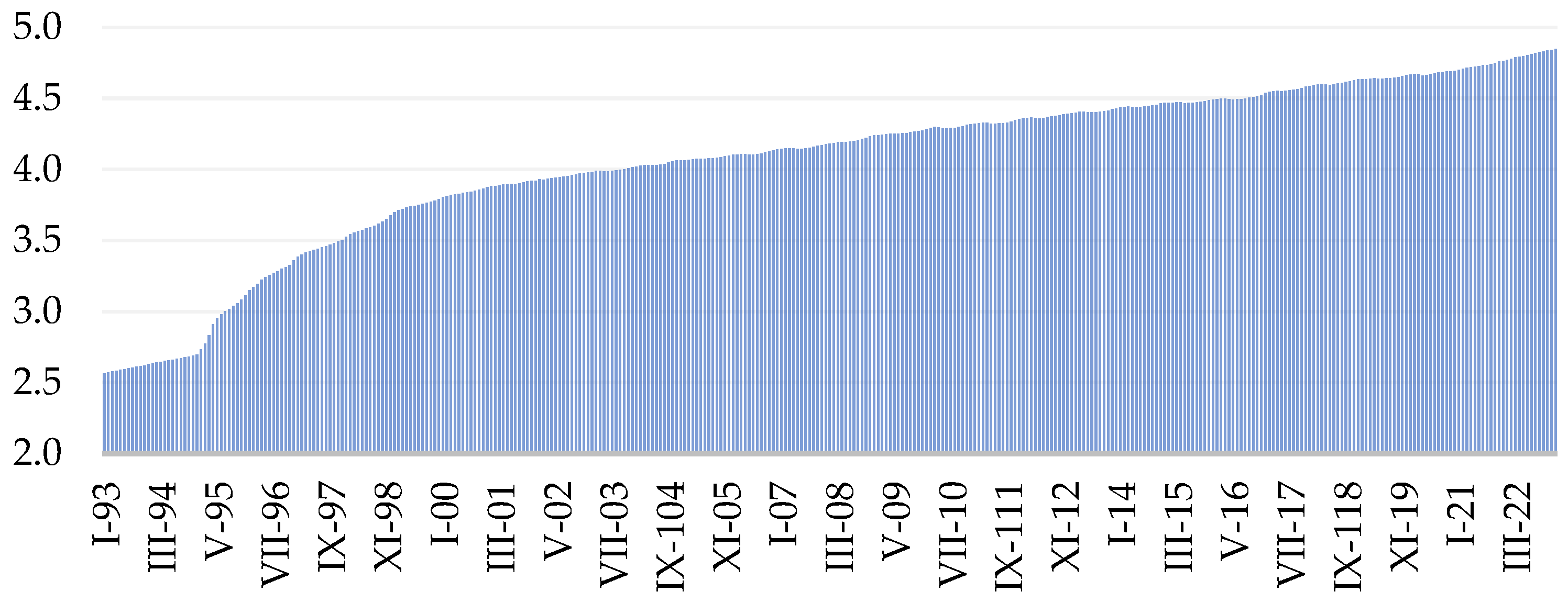
Figure 1. Behavior of the National Consumer Price Index in Mexico, in terms of natural logarithms, from January 1993 to January 2023 (INEGI 2013).
Economies 12 00021 g001
Figure 2. Behavior of the Global Economic Activity Index in Mexico, in terms of natural logarithms from January 1993 to January 2023 (INEGI 2013).
Economies 12 00021 g002
Figure 3. Summary of the 20 best models with Akaike Information Criterion (AIC, NARDL 12,9,10), with the application of the Eviews 12 package.
Economies 12 00021 g003
Figure 4. Behavior of the Global Economic Activity Index estimated by NARDL (12,9,10), with natural logarithms, 1994–2023 with the use of Eviews 12.
Economies 12 00021 g004
Figure 5. Stability diagnosis and CUSUM test with the NARDL model (12,9,10).
Economies 12 00021 g005
Figure 6. Shocks of asymmetric dynamic multipliers of l n I N P C t on l n I G A E t , using multiplier and the asymmetry identified with the NARDL model (12,9,10).
Economies 12 00021 g006
Table 1. Macroeconomic aggregates (impact channels on IGAE). Simple reduced-form model.
CoefficientsMacrofactors
WALCLShadow RatesGPUI
β 0 2.087563 *3.323633 *2.791119 *
β 1 0.726056 *0.287285 *0.413641 *
Γ i −0.010568 *−0.001492 *−2.68 × 10⁻⁵ *
The authors’ own elaboration using Eviews 12 (*) suggests significance with a confidence level of less than 1%.
Table 2. Stationarity analysis, order of integration, and nonlinearity.
lnINPCtlnIGAEt
Hypothesis Null: Unit Root (Prob > 0.05)t-Stat.Prob.Level (0,1)t-Stat.Prob.Level (0,1)
Augmented Dickey–Fuller (ADF test statistic)
* (Intercept)
Phillips–Perron (PP test statistic)
** (Intercept)
−3.6701
−4.7711
0.0049
0.0001
(0)−5.9783
−5.3803
0.0000
0.0000
(1)
1%−3.4484 −3.4490
5%−2.8693 −2.8697
10%−2.5710 −2.5711
KSS test
(Intercept) ***
6.1700 2.4884
1%0.2160 0.2160
5%0.1460 0.1460
10%0.1190 0.1190
BDS test ****
Significance (alpha) 0.0500 0.0500
p-value0.0000 0.0000
* Using Eviews 12 with data from Banxico, with an intercept and automatic selection of Schwarz Information Criterion (SIC), ** Newey–West Bandwidth, *** Matlab Kapetanios–Shin–Snell (KSS), **** R Brock–Dechert–Scheinkman–LeBaron test (BDSL test; or BDS test).
Table 3. Estimation results of the ARDL model.
VariableCoefficientProb.
Δ( l n I G A E 1 )−0.3674880.0000
Δ( l n I G A E 2 )−0.3476040.0000
Δ( l n I G A E 3 )−0.2666950.0000
Δ( l n I G A E 4 )−0.3161630.0000
Δ( l n I G A E 5 ) *0.0141780.8032
Δ( l n I G A E 6 )−0.1226330.0309
Δ( l n I G A E 7 ) *−0.0441060.4396
Δ( l n I G A E 8 )−0.1806730.0011
Δ( l n I G A E 9 )−0.1726220.0016
Δ( l n I G A E 10 )−0.2892570.0000
Δ( l n I G A E 11 )−0.2776660.0000
Δ( l n I N P C ) *−0.3553670.2788
Δ( l n I N P C 1 ) *−0.6858710.1114
Δ( l n I N P C 2 ) *0.4366110.3101
Δ( l n I N P C 3 )−0.8427150.0490
Δ( l n I N P C 4 )1.6901120.0001
Δ( l n I N P C 5 )−1.2327930.0046
Δ( l n I N P C 6 ) *−0.0714870.8696
Δ( l n I N P C 7 ) *−0.4591210.2931
Δ( l n I N P C 8 )1.2285970.0003
CointEq(−1)−0.0469640.0006
R-squared0.456934
Adjusted R-squared0.423719
Durbin–Watson stat1.779343
The authors’ own elaboration with the use of Eviews 12. (*) means that lagged variables are outside the 5% and 10% significance levels.
Table 4. Analysis of asymmetry (Ramsey test) *.
ValuedfProbability
t-statistic2.1967703240.0287
F-statistic4.825797(1, 324)0.0287
Likelihood ratio4.14504210.0233
* Own elaboration with the use of Eviews 12 through the diagnosis of residuals with the ARDL model.
Table 5. Estimation results of the NARDL model *.
Dependent Variable (NARDL):
l n I G A E t
Restricted Constant and No Trend, Dependent Variables with Long-Run Form:
Δ ( l n I G A E t )
Dependent Variable in Error Correction Model and Bound Test:
Δ ( l n I G A E t )
R-squared0.9836Asymmetric long-run
coefficients:
F-Bound test:
Adjusted R-squared0.9819 l n I N P C t + 0.1382F-static value *4.4224
F-statistic570.3971 (0.0063)Significance 10% I(1)Upper bound:
3.35
(0.0000) l n I N P C t −2.1238Significance 5% I(1)Upper bound:
3.87
Granger test. l n I N P C t causes l n I G A E t :
F-Statistic
9.9282
(0.00006)
(0.00012)Significance 2.5% I(1)Upper bound:
4.38
C.F.T.&Y test (****). l n I N P C t causes l n I G A E t :
Wald-Statistic
40.2252
(0.0001)
C4.30Serial correlation Lagrange multiplier, LM test ** (prob):(0.0002)
(0.0000)Heteroskedasticity test (prob.):(0.0000)
VariableCoefficients NARDL
(12,9,10)
VariableCoef. Long-Run FormVariableCoef. Error Correction Model
l n I G A E 1 0.5338 l n I G A E 1 −0.1138CointEq(−1)−0.1138
(0.0000) (0.0091) (0.0000)
l n I G A E 2 0.1172 l n I N P C 1 + 0.0157Δ( l n I G A E 1 )−0.3534
(0.0580) (0.0903) (0.0000)
l n I G A E 3 0.0196 l n I N P C 1 −0.2417Δ( l n I G A E 2 )−0.2352
(0.7555) (0.0347) (0.0000)
l n I G A E 4 −0.1232Δ( l n I G A E 1 )−0.3524Δ( l n I G A E 3 )−0.2156
(0.0507) (0.0000) (0.0001)
l n I G A E 5 0.3799Δ( l n I G A E 2 )−0.2352Δ( l n I G A E 4 )−0.3369
(0.0000) (0.0001) (0.0000)
l n I G A E 6 −0.0396Δ( l n I G A E 3 )−0.2156Δ( l n I G A E 5 )0.0430
(0.5421) (0.0004) (0.4528)
l n I G A E 7 −0.0005Δ( l n I G A E 4 )−0.3369Δ( l n I G A E 6 )0.0034
(0.9994) (0.0000) (0.9535)
l n I G A E 8 −0.1706Δ( l n I G A E 5 )0.0430Δ( l n I G A E 7 )−0.0034
(0.0058) (0.4900) (0.9535)
l n I G A E 9 0.0536Δ( l n I G A E 6 )0.0034Δ( l n I G A E 8 )−0.1672
(0.3898) (0.9565) (0.0024)
l n I G A E 10 −0.0941Δ( l n I G A E 7 )−0.0034Δ( l n I G A E 9 )−0.1136
(0.1275) (0.9556) (0.0375)
l n I G A E 11 −0.0506Δ( l n I G A E 8 )−0.1672Δ( l n I G A E 10 )−0.2078
(0.4094) (0.0044) (0.0001)
l n I G A E 12 0.2584Δ( l n I G A E 9 )−0.1136Δ( l n I G A E 11 )−0.2584
(0.0000) (0.0494) (0.0000)
l n I N P C + −0.6648Δ( l n I G A E 10 )−0.2078Δ( l n I N P C + )−0.6648
(0.0543) (0.0002) (0.0457)
l n I N P C 1 + −0.2182Δ( l n I G A E 11 )−0.2584Δ( l n I N P C 1 + )−0.8988
(0.7587) (0.0000) (0.0414)
l n I N P C 2 + 1.6302Δ( l n I N P C + )−0.6648Δ( l n I N P C 2 + )0.7315
(0.0346) (0.0543) (0.0986)
l l n I N P C 3 + −1.5519Δ( l n I N P C 1 + )−0.8988Δ( l n I N P C 3 + )−0.8204
(0.0441) (0.0424) (0.0614)
l n I N P C 4 + 2.0586Δ( l n I N P C 2 + )0.7315Δ( l n I N P C 4 + )1.2382
(0.0069) (0.1002) (0.0045)
l n I N P C 5 + −2.3017Δ( l n I N P C 3 + )−0.8204Δ( l n I N P C 5 + )−1.0634
(0.0025) (0.0629) (0.0147)
l n I N P C 6 + 1.3860Δ( l n I N P C 4 + )1.2382Δ( l n I N P C 6 + )0.3226
(0.0692) (0.0047) (0.4602)
l n I N P C 7 + −0.6907Δ( l n I N P C 5 + )−1.0634Δ( l n I N P C 7 + )−0.3681
(0.3658) (0.0152) (0.3996)
l n I N P C 8 + 1.0615Δ( l n I N P C 6 + )0.3223Δ( l n I N P C 8 + )0.6934
(0.1350) (0.4625) (0.0446)
l n I N P C 9 + −0.6934Δ( l n I N P C 7 + )−0.3681Δ( l n I N P C )5.4293
(0.0462) (0.4020) (0.0001)
l n I N P C 5.4293Δ( l n I N P C 8 + )0.6936Δ( l n I N P C 1 )1.1119
(0.0001) (0.0462) (0.4267)
l n I N P C 1 −4.5591Δ( l n I N P C )5.4293Δ( l n I N P C 2 )−1.3701
(0.0285) (0.0001) (0.3224)
l n I N P C 2 −2.4820Δ( l n I N P C 1 )1.11196Δ( l n I N P C 3 )−0.5182
(0.2333) (0.4405) (0.7081)
l n I N P C 3 1.8519Δ( l n I N P C 2 )−1.3701Δ( l n I N P C 4 )3.7905
(0.6813) (0.3329) (0.0065)
l n I N P C 4 4.3087Δ( l n I N P C 3 )−0.5182Δ( l n I N P C 5 )−3.0522
(0.0383) (0.7137) (0.0304)
l n I N P C 5 −6.4827Δ( l n I N P C 4 )3.7905Δ( l n I N P C 6 )−3.6844
(0.0012) (0.0084) (0.0087)
l n I N P C 6 −0.6322Δ( l n I N P C 5 )−3.0522Δ( l n I N P C 7 )−0.8176
(0.7666) (0.0363) (0.5633)
l n I N P C 7 2.8668Δ( l n I N P C 6 )−3.6844Δ( l n I N P C 8 )5.2600
(0.1776) (0.0107) (0.0002)
l n I N P C 8 6.0776Δ( l n I N P C 7 )−0.8176Δ( l n I N P C 9 )1.9680
(0.0041) (0.5746) (0.1551)
l n I N P C 9 −3.2920Δ( l n I N P C 8 )5.2600
(0.1241) (0.0003)
l n I N P C 10 −1.9680Δ( l n I N P C 9 )1.9680
(0.1720) (0.1720)
C0.4900C0.4900
(0.0071) (0.0071)
Model SpecificationFisher-Type Test statistics (B-H Coint. test) ***Coint.
Decision
EG-J5%
critical value
EG-J-BG-Bo5%
critical value
lnigae = f (lninpc)23.83578111.22955.13196521.931Cointegrated
* Own elaboration with the use of Eviews 12. The values in parentheses are the p-values of the NARDL econometric model. * The value is compatible with the t-Bounds distribution. ** Breush Godfrey test. *** Bayer–Hanck test, with the use of Stata. **** Cumulative Fourier Toda and Yamamoto Causality test, with the use of R.
Table 6. Optimization of the long-run form ( l n I G A E t ) * with stepwise regression.
VariableCoefficientProb.
C0.5422 = c(1) 0.0008
l n I G A E 1 −0.1273 = c(2)0.0011
l n I N P C 1 + 0.0184 = c(3)0.0411
l n I N P C 1 −0.2661 = c(4)0.0109
Δ( l n I G A E 5 )0.1135 = c(5)0.0220
Δ( l n I G A E 7 )0.0950 = c(6)0.0423
Δ( l n I G A E 6 )−4.7372 = c(7)0.0005
Δ( l n I N P C + )−1.1511 = c(8)0.0000
Δ( l n I N P C 9 )2.6416 = c(9)0.0560
Δ( l n I N P C 8 )3.4768 = c(10)0.0113
Δ( l n I G A E 11 )−0.2466 = c(11)0.0000
Δ( l n I G A E 1 )−0.3624 = c(12) 0.0000
Δ( l n I G A E 10 )−0.1821 = c(13)0.0001
Δ( l n I G A E 2 )−0.2539 = c(14)0.0000
Δ( l n I G A E 4 )−0.2810 = c(15)0.0000
Δ( l n I G A E 5 )−3.7702 = c(16)0.0051
Δ( l n I G A E 3 )−0.2264 = c(17)0.0001
Δ( l n I N P C )4.3162 = c(12)0.0018
Δ( l n I N P C 8 + )0.4792 = c(13)0.0339
* Own elaboration with the use of Eviews 12.
Table 7. Wald test to estimate errors with stepwise regression *.
Equation: STEP_UNIDI Long Run:
c(3) and c(4)
Short Run:
c(5) to c(13)
Test StatisticValuedfProbab.ValuedfProbab.
t-statistic4.07283290.00013.84723290.0001
F-statistic16.5881(1, 329)0.000114.8008(1, 329)0.0001
Chi-square16.588110.000114.800810.0001
* Own elaboration with the use of Eviews 12.
Disclaimer/Publisher’s Note: The statements, opinions and data contained in all publications are solely those of the individual author(s) and contributor(s) and not of MDPI and/or the editor(s). MDPI and/or the editor(s) disclaim responsibility for any injury to people or property resulting from any ideas, methods, instructions or products referred to in the content.