1. Introduction
Climate change caused by the increase in carbon dioxide emissions (CO
2) is one of the biggest concerns in the European region (
Bianco et al. 2019). CO
2 emissions are the most significant contributor to increased greenhouse gas emissions (GHGs), contributing 77% of GHGs. In contrast, other gases such as methane (CH
4), nitrous oxide (N
2O), and ozone (O
3) contribute with 14%, 8%, and 1%, respectively (e.g.,
Koengkan and Fuinhas 2021a,
2021b;
Khan et al. 2014).
Several initiatives have emerged to mitigate climate change (e.g., the United Nations Framework Convention on Climate Change (UNFCCC), the Earth Summit (1992), the Kyoto Protocol (1997), the 21st Conference of the Parties (COP 21) (2015), and the 26th Conference of the Parties (COP 26) (2021)). These initiatives aim to substantially limit the increase in temperature levels during this century to lower than 2 °C and limit that increase to 1.5 °C. These initiatives will take temperatures to pre-industrial levels. In addition, all countries that align with this agreement will move towards a low-carbon economy. Indeed, as has long been known, global GHGs, mainly CO
2 emissions, have been increasing since the 1970s (e.g.,
World Bank Open Data 2022;
Koengkan and Fuinhas 2021b).
However, from 1990 to 2016, these emissions grew dramatically, and in 1990, CO
2 emissions were 3.0991 (metric tons per capita) and reached 4.6807 (metric tons per capita) in 2016. During this period, these emissions grew from 33 megatons of CO
2 equivalent (MtCO2eq) in 1990 to 47 MtCO2eq in 2016, an annual increase of 1.5% during this period (
Bárcena et al. 2019). The energy, industry, transport, and building sector have increased emissions since the 2000s. In 2010 the energy sector contributed 25%, AFOLU (agriculture, forestry and other land use) 24%, industry 21%, transport 14%, other energy sources 10%, and the building sector contributed 6% to this growth (
Koengkan et al. 2020).
Most of these emissions are caused by the production of electricity and heat, which emanate from the industrial and residential sectors. GHGs come about through direct emissions from fossil fuel combustion for providing power, cooling, heating, and cooking (
Khan et al. 2014). As stated above, in 2010, energy consumption was responsible for 25% of global GHGs. The growth in global energy use is accountable for increasing CO
2 emissions. Energy use has been rising since the 1970s when energy use was 1337.00 (kg of oil equivalent per capita) in 1971 and reached 1897.25 in 2016 (e.g.,
World Bank Open Data 2022;
Koengkan and Fuinhas 2021a).
Indeed, 94% of this energy use in 1970 came from fossil fuels worldwide, and only 6.45% came from renewable energy. However, in 2016, the contribution of fossil fuels decreased slightly, reaching 85% of the total energy use. Indeed, this reduction is related to the increase in the share of renewable energy sources, which reached 14.35% in 2016 (
Our World in Data 2022).
In the European region, CO
2 emissions in 1971 were 8.0244 (metric tons per capita) and reached a value of 6.4684 (metric tons per capita) in 2016 (
World Bank Open Data 2022). Therefore, between 1990 and 2004, these emissions in the European region remained relatively unchanged. However, due to the 10.8% decrease in primary energy consumption, CO
2 emissions dropped sharply between 2005 and 2016 (
IEA 2020). For example, in 1990 the energy consumption was 1641 million tonnes of oil equivalent (Mtoe), while in 2004 it had already reached 1789 Mtoe. However, between 2005 and 2016, this consumption decreased and fell to 1598 Mtoe in the year 2016. The energy efficiency improvements that increased the share of renewable energy sources in the energy matrix and the changes in climate conditions were the causes for this decrease in the primary energy consumption between 2005 to 2016 for most European region countries (e.g., the
European Environment Agency 2019;
Eurostat 2020).
In the European region, 93% of this energy use in 1970 came from fossil fuels, and only 6.90% came from renewable energy. However, in 2016 this value decreased slightly, reaching 75% of total energy use. Indeed, this reduction is related to the increase in the share of renewable energy sources in energy use, where 25% was reached in 2016 (e.g.,
Our World in Data 2022;
Koengkan and Fuinhas 2021b).
As has long been known, various drivers have been influencing the increase of CO
2 emissions. Economic growth, globalisation, trade, financial liberalisation, urbanisation, population growth and energy prices have gained notoriety. However, the literature has given little consideration to a possible relationship between the obesity epidemic problem and the increase in environmental degradation. To the best of our knowledge, the first study to address the link between obesity and climate change was made by
Edwards and Roberts (
2009). However, this link is very complex and is not exempt from criticism (e.g.,
Gallar 2010).
Nevertheless, the literature remains scarce and primarily focused on the effect of obesity on climate change via CO
2 emissions. Their connections are associated with oxidative metabolic demands, food production, and fossil fuels. The links between obesity and climate change also include processed foods from fast-food and multinational supermarket chains, multinational food corporations, food production on farms, transportation of goods, retail processing and storage of processed food. These approaches also emphasise that the intensive use of motor vehicles and modern household appliances reduces physical effort in the context of a sedentary lifestyle (e.g.,
Magkos et al. 2019;
Furlow 2013;
Viscecchia et al. 2012;
Breda et al. 2011;
Edwards and Roberts 2009).
Obesity is defined as abnormal or excessive fat accumulation that may impair health, that is, individuals that have a mean body mass index (BMI) ≥ 30.0, as defined by the World Health Organization (WHO). The organisation also defines ‘overweight’ as BMI ≥ 25.0 (
Our World in Data 2022). In 2016, about 39% (2.0 billion) of adults aged 18 years and older, 38% of men and 40% of women worldwide, were overweight or obese (
Our World in Data 2022). Indeed, this chronic disease is a significant risk factor for people with many other diseases.
The obesity epidemic has increased significantly over the past three decades. In 2014, over 600 million adults, or 13% of the total adult population, were classified as obese worldwide. Of these 600 million obese adults, 11% are men, and 15% are women (
Pineda et al. 2018). It is estimated that 25.6% of the total adult population (18 and over) can be classified as obese in the European region. This disease has almost doubled since the late 1980s. In 1985, the percentage of obese adults that are obese was 12.60%, and this value reached 23.30% in 2016 (
Our World in Data 2022). Indeed, it has hit the world’s richest countries, regardless of individuals’ income levels.
Indeed, the obesity epidemic is caused by several factors: genetic, social, economic, environmental, political, and physiological, which have interacted to varying degrees over time (
Wright and Aronne 2012). Moreover, other factors, such as the globalisation process, urbanisation and technological progress, have caused an increase in the obesity epidemic (e.g.,
Fox et al. 2019;
Toiba et al. 2015;
Popkin 1998). The weight increase caused by the factors mentioned earlier contributes to making people physically less active (less physical activity also contributes to increasing obesity). Consequently, it leads to using more motorised vehicles and modern household appliances that reduce physical effort. In addition, it contributes to weight gain due to the lower caloric expenditure of individuals, as well as to increased consumption of processed foods, mainly produced by (i) multinational food companies, (ii) multinational supermarkets, and (iii) fast-food chains. All of these factors contribute to the increase in energy consumption from non-renewable energy sources and negatively impact the environment.
In the literature, the impact of the obesity problem on environmental degradation using a macroeconomic approach is not advanced in the literature. For this reason, this investigation opted to use similar studies related to this topic (e.g.,
Koengkan and Fuinhas 2021b;
Cuschieri and Agius 2020;
Magkos et al. 2019;
Swinburn 2019;
Webb and Egger 2013;
Viscecchia et al. 2012;
Breda et al. 2011;
Davis et al. 2007;
Higgins 2005). These investigations pointed out that the obesity problem increases environmental degradation. However, none of these studies realised an analysis using a macroeconomic approach. They used the percentage of adults that are overweight or obese as a proxy for obesity and CO
2 emissions as a proxy for environmental degradation as well as the quantile via moments (QvM) method. Furthermore, these studies do not use the urban population and globalisation as independent variables. Moreover, none of these studies investigated the European countries. That is, there are gaps in the literature that need to be filled.
In order to fill the gaps that were mentioned above, this investigation will identify the macroeconomic effect of the obesity epidemic on environmental degradation. Indeed, to identify this effect, this empirical investigation will study a group of thirty-one countries from the European region between 1991 to 2016 that have experienced a rapid increase in the obesity epidemic and social, economic, and environmental transformations. Certainly, to carry out this empirical investigation, the quantile via moments (QvM) approach, which
Machado and Silva (
2019) developed, will be used.
This investigation will introduce a new analysis regarding the macroeconomic impact of the obesity problem on environmental degradation in European countries. This topic of research has never been approached before in the literature. Therefore, this study can open new opportunities for studying the correlation between obesity and environmental degradation through a macroeconomic aspect. Furthermore, this investigation is innovative in that it uses econometric and macroeconomic approaches to identify the possible effect of the obesity problem on ecological degradation. It is the first time this methodology approach has been employed in this kind of investigation.
Moreover, this investigation will contribute to the literature for several reasons: (i) it introduces a new analysis regarding the effect of the obesity epidemic on environmental degradation in European countries. This topic of investigation is new and can open new issues of inquiry regarding the relationship between health and the environment using a macroeconomic approach; (ii) this investigation will contribute to introducing the QvM model; and (iii) the results of this study will help governments and policymakers develop more initiatives to reduce the obesity problem in the European countries, in addition to policies to reduce the consumption of non-renewable energy sources and environmental degradation.
This study is ordered as follows.
Section 2 presents the literature review regarding the effect of the obesity epidemic on environmental degradation.
Section 3 provides the data and the methodology approach.
Section 4 presents the results and a brief discussion. Finally,
Section 5 presents the conclusions and limitations of the study.
2. Literature Review
Koengkan and Fuinhas (
2021b) investigated the impact of the overweight epidemic on energy consumption in thirty-one countries in the European region from 1990 to 2016. The authors find that being overweight increases the consumption of energy from fossil fuels and consequently increases the emissions of CO
2. Moreover, according to the authors, the increase in energy consumption and CO
2 emissions by the overweight epidemic is related to the increased consumption of processed foods from fast-food and multinational supermarket chains and multinational food corporations. Indeed, this process positively affects farm production, fast-food and multinational supermarket chains, and multinational food corporations to attend to the demand for processed foods. This increase affects the consumption of energy from non-renewable energy sources.
Magkos et al. (
2019) explored the effect of obesity on climate change. The authors point out that this health problem can aggravate climate change with increased CO
2 emissions in three ways: (i) oxidative metabolic demands; (ii) food production; and (iii) fossil fuels use. The increase of oxidative metabolic demands caused by the higher body mass associated with obesity is responsible for 7% of total GHGs. Indeed, the rise in production driven by the need to provide higher energy caloric intake is responsible for 52% of total GHGs. In contrast, the increase in fossil fuel consumption caused by transport and food production is responsible for 41% of these emissions. Thus, the authors estimated that the obesity epidemic adds the equivalent of 700 megatons of extra carbon dioxide to emissions per year or about 1.6% of the total global emissions. This idea is also shared by
Swinburn (
2019), who investigated the same topic.
Other authors also share similar ideas, such as
Breda et al. (
2011), who studied the relationship between climate change and obesity in four regions of Karakalpakstan in Uzbekistan. According to the authors, there is strong evidence that being overweight contributes more to climate change, where overweight influences food consumption and production. Those categories contribute more to climate change by consuming processed foods from fast-food and multinational supermarket chains, multinational food corporations, and farms. The authors add that the food sector accounts for 7% of CO
2 emissions, 43% of CH
4 emissions, and 50% of N
2O emissions produced across the entire economy.
Viscecchia et al. (
2012) investigated the relationship between obesity and climate change in Italy. The authors opted to use the ordinary least squares method to undertake this investigation. The authors found that the increase in food consumption with low energy content has a twofold effect on reducing obesity and climate change mitigation. Moreover, the increase in food consumption with low energy caloric content reduces the obesity rate from 9.68 to 7.04% and avoids 5,406,000 tons of CO
2 emissions per year.
Cuschieri and Agius (
2020) investigated the link between diabetes caused by obesity and climate change. The increase in the demand for processed food caused by obesity also has an adverse effect on the climate. The authors highlight that this effect is caused by the increased transportation of goods, retail processing, and processed food storage.
Webb and Egger (
2013) also studied the link between obesity and climate change and point out that some behaviours connected with obesity also affect emissions of GHGs associated with climate change. The authors show that consuming processed food and non-renewable energy sources results from intensive motor vehicles and modern household appliances that reduce physical effort.
Davis et al. (
2007) investigated the interactions between cars, obesity, and climate change in the United Kingdom from 1974 to 2004. Their results precede the idea developed later by
Webb and Egger (
2013). According to the authors, the intensive use of motor vehicles in the United Kingdom has reduced physical activity and increased obesity and CO
2 emissions by increasing non-renewable energy sources.
Higgins (
2005), in an investigation that investigated whether “exercise-based transportation reduces oil dependence, carbon emissions and obesity”, points out that the use of the automobile as a means of transport also contributes to a sedentary lifestyle and the obesity epidemic and poor health. The author adds that these problems consume 27% of global oil production and produce 25% of global carbon emissions.
The summary of the literature presented in this section has discussed some of the most consequential investigations that directly approached the impact of obesity on environmental degradation and similar investigations. However, none of these studies realised an analysis using a macroeconomic approach. Instead, they used the percentage of adults that are overweight or obese as a proxy for obesity and CO2 emissions as a proxy for environmental degradation, as well as the quantile via moments (QvM) method. Furthermore, these studies do not use the urban population and globalisation as independent variables. Moreover, none of these studies investigated the European countries. Therefore, there are gaps in the literature that need to be filled. The following section will show the data and methods used in this investigation.
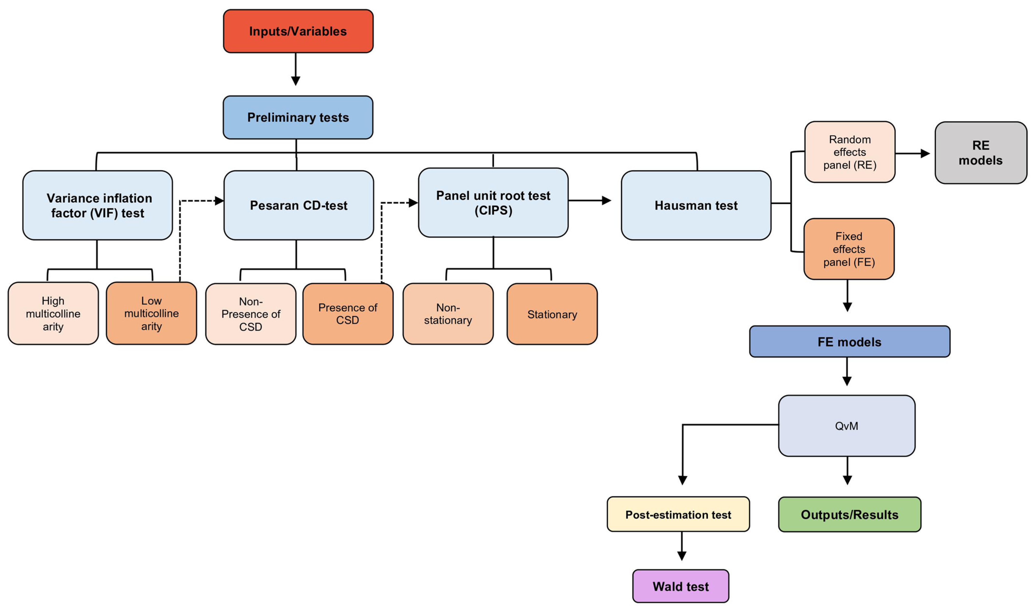
4. Results and Discussions
As previously explained, this section will present the results and the possible explanations for the macroeconomic impact of the obesity epidemic on environmental degradation. The preliminary tests indicated that the variables used have characteristics such as (i) low-multicollinearity among independent variables (as shown in
Table A1 in
Appendix A); (ii) cross-sectional dependence in the logs of variables (as shown in
Table A2 in
Appendix A); (iii) variables with orders of integration borderline I(0) and I(1) (as shown
Table A3 in
Appendix A); and (iv) the presence of panel fixed-effects (as shown
Table A4 in
Appendix A). This last result is significant because fixed effects are required in the QvM model. Therefore, the fixed-effects estimator is the most suitable for accomplishing this empirical analysis. Therefore, the empirical results of these tests are vital to identifying the characteristics of the group of countries under study and the possible methodologies to be applied.
The next step after the preliminary tests is to carry out the model regression. The 25th, 50th, and 75th quantiles were calculated to assess the non-linearities of the effect of the obesity epidemic on environmental degradation. We utilised these quantiles to simplify the exhibition of empirical results. Furthermore, we used several quantiles (e.g., 5th, 10th, 15th, and others). It can be seen that there is no information loss, as all independent variables pointed to the same effect of the dependent variable.
Moreover, a dummy variable was added to the model because, during the analysis, the European countries suffered some shocks, such as economic and political. Indeed, if these shocks are not considered, it could produce inaccurate results and misinterpretations during model regression. Therefore, this empirical analysis added dummy variables that represent these shocks. In the literature, the inclusion of dummy variables needs to follow the following triple criterion of choice developed by
Fuinhas et al. (
2017). For example, (i) the potential relevance of recorded economic and political events at the country level; (ii) the occurrence of international events known to have disturbed the European countries; and (iii) a significant disturbance in the estimated residuals. Therefore, the dummy variables added to the model regression are IDEUROPE_2015 (Europe, the year 2015). The dummy variables called “IDEUROPE_2015” represent a decrease in all countries’ GDP in the model. This event was caused by the persistent effects of the European debt crisis (often also referred to as the eurozone crisis or the European sovereign debt crisis (
Koengkan and Fuinhas 2021a).
Table 5 below shows the QvM model regression results with the dummy variable’s inclusion. The QvM model results without including the dummy variable can be seen in
Table A5 in
Appendix A.
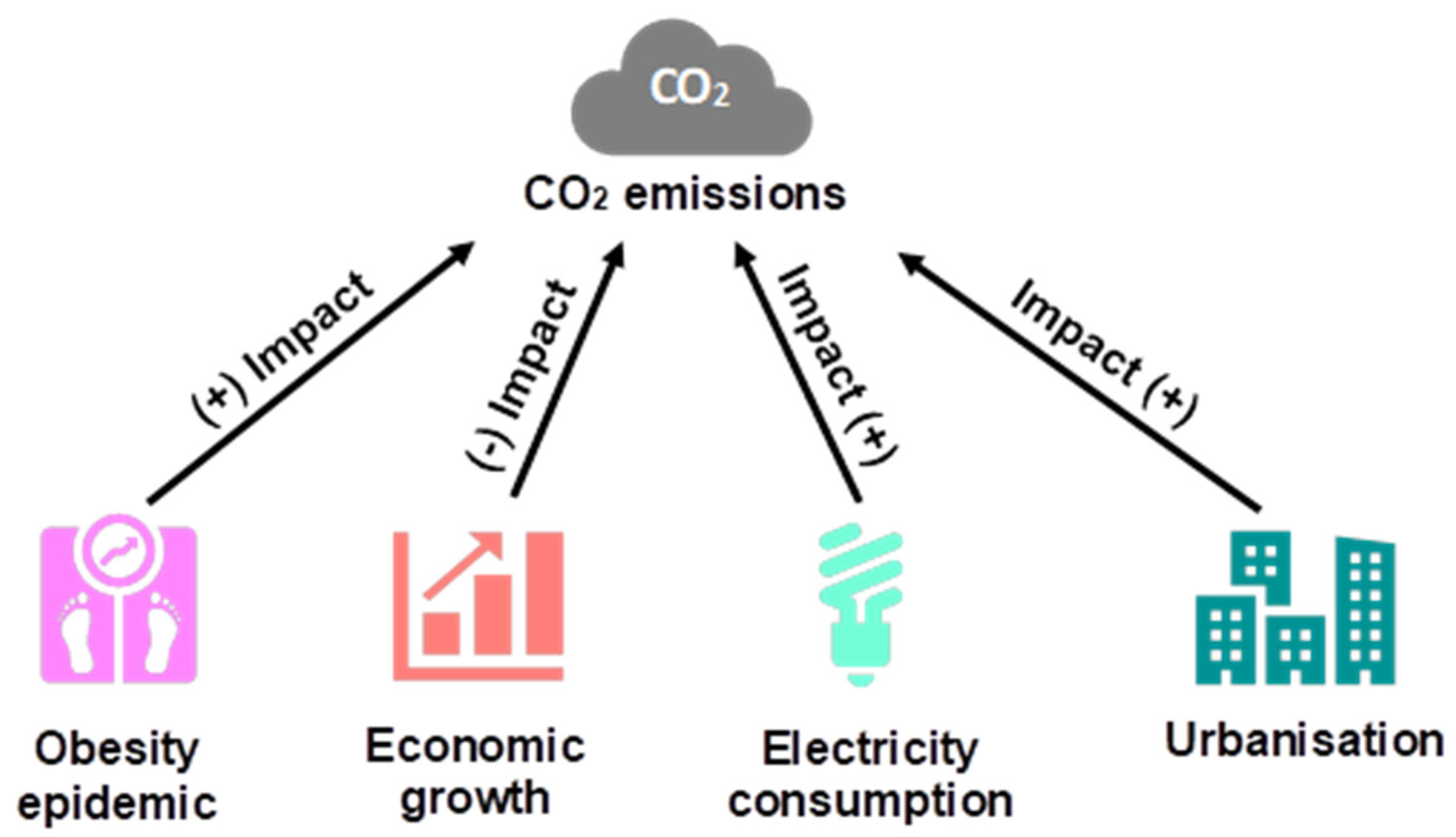
The QvM model regression results indicate that in the 25th, 50th and 75th quantiles, the obesity epidemic, electricity consumption, and urbanisation process increase CO
2 emissions. That is, they encourage environmental degradation by increasing CO
2 emissions. Nevertheless, economic growth decreases emissions of CO
2 in the European region. Moreover, the results from the QvM model also show non-linear behaviour. The estimated coefficients values vary as we go up (or down) in the quantiles’ regression. Thus, the empirical results answer the central question of our empirical investigation. Moreover, the post-estimation tests (e.g., the Modified Wald test) indicate that the estimator of this study is adequate (as shown in
Table 6 below).
After finding the positive effect of the obesity epidemic on environmental degradation, it is necessary to ascertain whether the results found by the QvM model regression are reliable and robust when we perform a change in the econometric method approach. Indeed, this approach to finding if the model is robust or not was previously used by
Koengkan et al. (
2020) and
Fuinhas et al. (
2017).
After identifying that the obesity epidemic encourages environmental degradation by increasing CO
2 emissions, the next step is to answer the following question: What is the possible explanation for this phenomenon? One possible way of explaining this effect is that the obesity epidemic is caused by the increased consumption of processed foods from multinational food corporations, fast-food chains and multinational supermarket chains, as well as the food production on farms, as indicated by some authors (e.g.,
Koengkan and Fuinhas 2021b;
Fox et al. 2019;
Gerbens-Leenes et al. 2010;
Popkin 1998). The increased consumption of processed foods from multinational food corporations and farms will positively affect energy consumption from non-renewable energy sources.
Another explanation for this phenomenon is related to the reduction of outdoor activities, which exacerbates the problem of obesity. Consequently, this reduction will encourage intensive motorised transportation, screen-viewing leisure activities, and the use of home appliances, as indicated by some authors (e.g.,
Koengkan and Fuinhas 2021b;
Bell et al. 2002;
Sobal 2001). Indeed,
Koengkan and Fuinhas (
2021b) also add that the increase in the use of home appliances and motorised transportation has implications for the energy demand from fossil fuel energy sources, where the consumption of these kinds of sources increases considerably.
Additionally, the positive impact of the obesity epidemic on CO
2 emissions is also indirectly related to economic growth, globalisation, and urbanisation. Therefore, the levels of obesity have been related to increasing economic activity, where economic development causes effects on dietary changes (e.g.,
Springmann et al. 2016). Indeed, the transition from low to high income caused by this process tends to induce some individuals to consume fatty and energy-dense foods of animal origin. Therefore, the increase in income contributes to the rise in obesity levels, except in countries where home-produced food is predominant (e.g.,
Roskam et al. 2010;
Gerbens-Leenes et al. 2010).
The globalisation process also causes an increase in obesity by the dietary changes. According to
Popkin (
1998),
Fox et al. (
2019),
Koengkan and Fuinhas (
2021b) and
Koengkan et al. (
2021), the process of globalisation will contribute to the food chain extension. As mentioned above, this extension will enable economies of scale in food production processes. Consequently, the economies of scale in food production processes will allow a diet rich in energy-caloric foods. Food consumption with high sugar and salt contents is less expensive and accessible to lower-income classes. Moreover, the unhealthy supply of processed foods is related to the increase in multinational food companies, supermarkets, and fast-food chains caused by globalisation.
The urbanisation process also plays a role in the increase in the obesity problem. The process of urbanisation allows better accessibility to food due to supermarkets, multinational supermarkets, and fast-food chains offering a ready supply of processed foods, which consequently causes the decline of farm stands and open markets with healthier foods (
Reardon et al. 2003). This same process also exposes people to the mass media marketing of food and beverages that influence traditional diets (
Hawkes 2006). Moreover, urbanisation increases car use and reduces walking or biking for transportation or leisure, contributing to obesity, and obesity increases car use. Moreover, all these explanations align with the findings of
Koengkan and Fuinhas (
2021b). They found that economic growth, globalisation, and urbanisation positively affect the overweight problem in the European region. They consequently encourage energy consumption from non-renewable energy sources and subsequently increase CO
2 emissions/environmental degradation. Furthermore, the explanations above align with the results from the complementary analysis that this investigation carried out (as shown in
Table A6, in
Appendix A).
Indeed, the positive effect of electric power consumption on CO
2 emissions could be related to some factors highlighted in this empirical investigation. On the one hand, it can be linked to electricity consumption in groups of not environmentally responsible countries. Consequently, electricity generation from fossil fuels is linked with increases in CO
2 emissions. These findings may also signal that the panel of countries under study could depend on fossil fuel sources for economic growth. On the other hand, it may be linked to the inefficiency of renewable energy policies that stimulate the development and consumption of renewable energy sources. Several authors have already found this impact (e.g.,
Fuinhas et al. 2021;
Ozcan et al. 2020;
Muhammad et al. 2020;
Adedoyin et al. 2020;
Koengkan and Fuinhas 2021b;
Yazdi and Dariani 2019;
Salahuddin et al. 2019;
Fuinhas et al. 2017).
However, the negative effect of economic growth on CO2 emissions could be related to some factors highlighted in this empirical investigation. A justification for the negative impact can be linked to a strong depression/recession affecting people’s consumption behaviour. Accordingly, it affected energy-intensive sectors, electricity consumption, and, finally, the emissions of CO2. A U-shaped relationship between economic growth and CO2 emissions could be another possible explanation for this negative impact. An increase in economic growth initially leads to a decline in CO2 emissions levels, consequently reaching a threshold. Indeed, economic activity intensifies environmental degradation. Indeed, the country’s industrialisation increases pollution. The policies limiting the levels of industrial pollution can be another explanation. Those policies promote the embracing of environmentally friendly techniques and processes of production.
Consequently, environmentally friendly technologies were promoted, and this promotion contributes to producing and consuming renewable energy by industries and families. However, some authors found a negative impact on economic growth and CO
2 emissions (e.g.,
Koengkan and Fuinhas 2021b;
Muhammad et al. 2020;
Aye and Edoja 2017).
Moreover, the positive effect of urbanisation on CO
2 emissions could be related to increased urban populations, positively affecting the demand for energy from fossil fuel energy sources, households, the transport sector and industries. Additionally, this positive effect could be related to the low energy efficiency improvement caused by the slow introduction of new energy technologies, low diversification of energy sources and low environmental regulation efficiency. It encourages industries’ and families’ acquisition of environmentally friendly technologies (
Koengkan and Fuinhas 2021b).
Figure 2 below summarises the effect of independent variables on the dependent variable.
This section showed the results from the primary model and the robustness check, the possible explanations for the impact of the obesity epidemic on environmental degradation, and a brief explanation of the impact of other variables. The next section will show the conclusions of this experimental investigation.
5. Conclusions
This empirical investigation approached the macroeconomic effect of the obesity epidemic on environmental degradation using CO2 emissions as a proxy in a panel of thirty-one European countries from 1991 to 2016. As stated above, the QvM model was used to carry out an empirical study. This study’s preliminary tests indicated that the variables used have low-multicollinearity characteristics, cross-sectional dependence in logarithms, and variables have I(0) or borderline I(1) order of integration, non-presence cointegration between the variables, and also fixed-effects.
The QvM and fixed-effect models regression results show that the obesity epidemic, electricity consumption, and urbanisation encourage environmental degradation by increasing CO2 emissions. At the same time, economic growth decreases the emissions of CO2 in the European region. Indeed, the post-estimation test results for the QvM model indicate that this study’s estimator is adequate.
The obesity epidemic increases the environmental degradation problem in three ways. First, the obesity epidemic is caused by increased consumption of processed foods from fast-food and multinational supermarket chains and multinational food corporations. The increase in food production will positively impact fossil fuel energy sources’ energy consumption. Second, obesity reduces physical and outdoor activities, increasing the intensive use of motorised transportation, home appliances, and screen-viewing leisure activities, consequently increasing energy consumption from non-renewable energy sources. Finally, a third possible way can be related indirectly to economic growth, globalisation, and urbanisation. This empirical evidence leads to a supplementary research question: What can be done to reverse the influence of the obesity epidemic on environmental degradation in the European region?
Several initiatives need to be created to reduce the effect of the obesity epidemic on environmental degradation. The first initiative is related to policies that reduce the sale of foods with high calorie-energy close to schools; the second initiative is to create policies that restrict the sale and consumption of unhealthy foods through taxation. Unhealthy food will cost more with the introduction of taxes and, consequently, encourage healthier foods. The third initiative is related to developing policies that encourage the generalised practice of physical activity and its importance. The fourth initiative is related to reducing lobbying by multinational food corporations through policies encouraging local producers. Finally, the fifth and last initiative is associated with creating policies that encourage the food sector to produce foods that are more healthy and have the least possible impact on the environment.
However, this problem is not limited to reducing the obesity problem. It is necessary to change production and consumption in the European region. Indeed, several initiatives have already been implemented to reduce the consumption of non-renewable energy in the region. However, it is essential to do more to reverse this situation. For example, policymakers need to create more measures to reduce the barriers to products and technologies that improve energy efficiency and produce green energy. This reduction could benefit households and industries by acquiring renewable energy technologies and reducing these products’ prices.
Regarding food production, it is necessary to introduce policies that encourage, (i) better productivity, where the efficiency improvements can lead to a 33% reduction in land use, a 12% reduction in water use, and a 16% reduction in production emissions; (ii) reduce livestock emissions, where the increase in productivity and efficiency gains can reduce land use, feed requirements, and GHG emissions per gallon of milk or pound of meat; (iii) reduce the consumption of fertiliser, as the use of these substances emits nitrous oxide, a potent greenhouse gas (the introduction of techniques including nitrification inhibitors can replace applications of fertilisers); (iv) introduce renewable energy and energy efficiency technologies supported by fiscal and financial instruments that help farmers gain access to renewable energy and energy-efficient technologies; and (v) reduce waste and food loss, with support of fiscal and financial instruments to help farmers to improve their equipment and energy efficiency in farm buildings. In addition, these policies can reduce the consumption of fossil fuels and emissions.
This study is a kick-off regarding the effect of the obesity epidemic on environmental degradation and other aspects such as energy consumption, economic growth, and urbanisation. Therefore, this investigation is in the initial stages of maturation, which will supply a solid foundation for second-generation research regarding this topic.
Limitations of the Study
As we already know, this empirical investigation is not free of limitations. Indeed, the preliminary limitations of this empirical investigation stem from (i) the presence of a short period. In this investigation we used the period between 1991 and 2016. Indeed, this period was used due to data availability for the variable OBESE. Moreover, more time is necessary to capture the dynamic effects of the variables OBESE, EC, Y_PC, and UP; (ii) the inexistence of literature that approaches the macroeconomic effect of the obesity epidemic on environmental degradation. The lack of this kind of literature makes difficult the elaboration of deeper discussions regarding the results found; and (iii) the European countries are firmly integrated and are mainly developed ones. This former characteristic limits the generalisation of our results to diverse contexts.
The limitations mentioned above are usually found in investigations in their early stages of maturation. Developing second-generation studies regarding this topic is essential to overcoming these limitations. Despite the limitations in this investigation, this study could draw meaningful conclusions.


