Measuring the Effect of the Misery Index on International Tourist Departures: Empirical Evidence from Mexico

Abstract

Tourism’s capacity to alleviate poverty is one of the most important subjects in tourism studies, as tourism is capable of boosting economic growth and generating employment. On the other hand, it is known that lack of income and unemployment have negative effects on outbound tourism; however, the relationship between outbound tourism and poverty has been understudied. In this paper, we compute a vector autoregressive (VAR) model to analyze the relationship between tourist departures from Mexico and a modified misery index to measure the effect of the loss of well-being, measured in terms of this index, on the number of outbound tourists. The results indicate that increases in the misery index have negative effects on the number of outbound tourists. Conversely, there is no statistically significant effect of tourist departures on the misery index. The results also suggest that the depreciation of the national currency exerts a positive effect on the misery index. Finally, based on the historical decomposition analysis, it was verified that the misery index was not closely related to outbound tourism during the first COVID-19 wave.

1. Introduction

Inbound tourism is considered a main driver of economic growth. The tourism-led growth hypothesis, according to Rasool et al. (2021), is directly founded on the export-led growth hypothesis, which claims that economic growth can be boosted not only by way of increasing labor and capital but also by means of furthering exports. According to Hipsher (2017), tourism is a labor-intensive sector that benefits those with low levels of skill and education.

According to Sharma and Thapar (2016), tourism is among the most lucrative non-technology-based economic sectors, particularly in developing nations, as these types of countries frequently confront problems such as lack of capital, lack of employment opportunities, and poverty. Since tourism is considered to make an important contribution to economic growth, besides being recognized as an employment-generating sector, Weinz and Servoz (2013) consider it to have important potential for poverty reduction.

Conversely, outbound tourism spending is cataloged as an import for the country of origin, so its value is compared with the country’s export value (Mehran and Olya 2019). In this sense, outbound tourism, following Seetaram (2010), is considered to largely affect the economy in the opposite direction of inbound tourism in terms of economic growth and employment creation.

This study aims to investigate the relationship between the misery index and tourist departures in Mexico. To achieve this goal, we computed an unrestricted vector autoregressive (VAR) model, which considers the compensated misery index (CMI), the multilateral real exchange rate, and the number of outbound tourists as endogenous variables. The main results of this model suggest, on the one hand, that the number of outbound tourists is diminished by increases in the CMI but, on the other hand, that tourist departures do not have a statistically significant effect on the CMI. In addition, the results show that, during the first wave of the COVID-19 pandemic, the CMI and tourist departures were not closely related.

We believe that this article contributes to the existing literature in the following ways. First, to the best of our knowledge, this is the first study documenting the relationship between poverty, in terms of the CMI, and tourist departures, as this subject has been traditionally studied from the perspective of inbound or domestic tourism. Second, this document contributes to closing the gap between studies on outbound and inbound tourism. In the same vein, we consider that it will be of interest to policymakers and tourism managers, as it provides statistical evidence that the misery index helps explain decreases in outbound tourism demand, and also that tourist departures have not had a statistically significant impact on the loss of well-being measured in terms of this index during the study period.

The remainder of this paper is organized as follows. In Section 2, we present the literature review, which is divided into two subsections: we first present a detailed literature review on the discomfort economic index and then review the links between outbound tourism and the misery index. Section 3 is also divided into two subsections, as we present the data and their sources and the VAR empirical design. In Section 4, we present the econometric results. Finally, in Section 5, the discussion and conclusions are presented.

2. Literature Review

2.1. Discomfort Economic Index

In its original form, according to Lechman (2009), Okun’s misery index $\left(MI\right)$ is calculated by simply adding the unemployment rate $\left(U\right)$ to the inflation rate $\left(\pi \right)$:

$$MI=U+\pi$$

(1)

The expression in Equation (1) was initially named the “discomfort economic index” (Lechman 2009). In 1980, U.S. President Ronald Reagan renamed it “the economic misery index” in “deriding” the previous U.S. president, Jimmy Carter (Lovell and Tien 2000).

Okun’s misery index probably constituted the first attempt to measure a population’s economic malaise in a single number (Cohen et al. 2014). It was conceived to measure the loss in general welfare and as an objective method to quantify economic malaise (Lechman 2009). In fact, this index endeavors to summarize the most evident costs for society, as unemployment prevents people from earning an income, whereas high inflation rates increase the cost of living by reducing purchasing power (Riascos 2009).

Most of the criticisms of the discomfort economic index are due to its simplicity, as it embodies an oversimplification of the socioeconomic problems affecting society (Lovell and Tien 2000; Riascos 2009). In fact, it is considered a simplified version of the social preference function over inflation and unemployment (loss function), as the loss function differs from the misery index in both its functional form and weights (Welsch 2007).

Given that Okun’s misery index considers only two macroeconomic indicators, according to Lovell and Tien (2000), it can be regarded as a “crude (dis)utility function”. Lovell and Tien argue that Okun implicitly supposed that the indifference curves describing people’s preferences for unemployment and inflation are straight lines with a slope equal to −1, implying that citizens’ aversion to such economic indicators is identical.

However, Winkelmann and Winkelmann (1998) found that unemployment has a strong negative impact on life satisfaction, claiming that non-pecuniary costs of unemployment are higher than pecuniary costs. Di Tella et al. (2001) demonstrated that unemployment has more negative effects on reported well-being than inflation, indicating that Okun’s misery index underweights the discontent generated by joblessness. Additionally, Asher et al. (1993) consider that variations in MI are policy-related, but it is not easy to attribute them to specific policy actions.

Despite the criticisms of its simplicity, Okun’s misery index is frequently used to examine social welfare (Riascos 2009). In fact, Grabia (2011) considers that such an index establishes a kind of poverty index due to the effects of unemployment and inflation on average citizens’ standards of living. Moreover, according to Riascos (2009), Okun’s misery index, as a poverty measure, should be considered an objective indicator, as it does not take into account the socioeconomic perception that persons or households have of themselves. Additionally, Riascos proposed including the MI among the monetary approaches to measure poverty, as monetary indicators of poverty are based on income’s capacity to guarantee the satisfaction of basic life conditions. Nonetheless, it is very important to mention that, according to Lechman (2009), MI is not a perfect measure of poverty, but its fluctuations reflect “changes in society’s economic performance”.

Additionally, this index has been applied in a vast number of ways; for example, Yang and Lester (1999) found that, in the case of the United States, Okun’s misery index is related to the number of suicides. In the case of Iran, Piraee and Barzegar (2011) found a long-term relationship between the misery index and economic crimes such as embezzlement, bribery, forgery, and drawing counterfeit checks. Özcan and Açıkalın (2015) found that in the case of Turkey, there is a relationship between lottery gambling and the misery index, arguing that people are more prompted to bet in lottery games during economic crises. Similarly, in the case of Turkey, Akçay (2017) found that the MI has a positive impact on remittance flows in both the short and long term. Wang et al. (2019) provided empirical evidence on the negative effects of the MI on economic growth in Pakistan.

There have also been numerous modifications to Okun’s misery index; for example, MacRae (1977) proposed that the loss of votes for the incumbent political party is a quadratic function of unemployment and inflation. Barro (1999) developed the so-called Barro misery index (BMI), which incorporates the interest rate and GDP; Barro argues that increases in the long-term interest rate and economic growth below the average also contribute to misery. Lovell and Tien (2000) suggest using the absolute value of the inflation rate; they consider that the effects of deflation are as “painful” as those of inflation. Ramoni-Perazzi and Orlandoni-Merli (2013) recommended adding employment in the informal sector to the measure, since joining this sector is frequently an immediate response by workers to subsistence problems, making informality a form of hidden unemployment to some extent. Cohen et al. (2014) developed a dynamic misery index using the expectation-augmented Phillips curve and Okun’s law. Murphy (2016) elaborated on a state misery index for the United States using data on regional pricing parities.

Based on the BMI, Hortalà and Rey (2011) calculated a “compensated misery index” by subtracting the economic growth rate $\left(\dot{y}\right)$ from Okun’s original misery index, as shown in Equation (2):

$$CMI=MI-\dot{y}$$

(2)

It is important to mention that Gaddo (2011) uses a similar specification of the misery index, simply calling it “modified Okun”. In this document, we use the abbreviation CMI to denote the expression in Equation (2) in reference to the name utilized by Hortalà and Rey (2011).

In this document, based on the idea that the MI represents a type of poverty index, we study the impact of CMI on Mexico’s international outbound tourism to approximate the effect of poverty on the decision to travel abroad. The CMI was selected among the different specifications of the misery index because the empirical findings suggest that all three CMI components are tourism-related, as will be discussed in the following subsection.

2.2. Outbound Tourism and Compensated Misery Index

According to the World Bank (2021),

“International outbound tourists are the number of departures that people make from their country of usual residence to any other country for any purpose other than a remunerated activity in the country visited”.

From an accounting perspective, international outbound tourists’ spending is classified as an import (Boullón 2009; Seetaram 2010), and income is among the main determinants of the import level (Sosa 2001). Moreover, tourism behaves as a luxury good (Álvarez 1996; Smeral 2003), which implies, by definition, that its income elasticity of demand will be greater than unity when income rises by 1% (Varian 1999).

Economic crises have a profound effect on the tourism sector since, as mentioned by Ramírez (1994), tourism is sustained by three basic factors: available time, desire to travel, and economic resources. According to Álvarez (1996), during phases of economic decline, tourism demand, measured as tourist spending, decreases more than proportionally with respect to the fall in the income level.

In general, countries with important proportions of outbound tourists have a high income level, as well as an adequate income distribution (Ascanio 2012). Effectively, the income level is likely to determine a strict upper limit for tourism demand, whereas the lack of a certain level of wealth prevents individuals or households from acquiring superior goods (Kim et al. 2012). Moreover, traveling abroad for tourism purposes usually takes place once basic needs have been met (Ascanio 2012; Panosso and Lohmann 2012).

Concerning unemployment, Sánchez (2019) provided empirical evidence of a bidirectional relationship between tourism GDP growth and the unemployment rate; on the one hand, tourism GDP growth helps reduce the unemployment rate, but on the other, increases in the unemployment rate diminish the growth of tourism GDP. Alegre et al. (2019) found that high levels of unemployment increase the probability of not going on vacations, as unemployment represents an indicator of the current economic situation, in addition to influencing future expectations of income and employment.

Inflation deteriorates the purchasing power of a currency; such deterioration can incline consumers toward basic goods and services, thus postponing the decision to travel for tourism purposes, as well as the acquisition of other non-essential goods and services (Dominé 2014). However, tourism purchases are usually made in advance of their actual consumption; therefore, past values of prices and exchange rates are better at explaining tourism demand than current values (Stabler et al. 2009).

On the other hand, since outbound tourism is regarded as a form of import, its effects on the economy are considered to be the opposite of those generated by inbound tourism in terms of economic growth, the reduction of unemployment, and the generation of foreign currencies (Seetaram 2010). However, outbound tourists also contribute to the economy as they spend money in their residence country when preparing to travel; this often includes spending on airlines, passports, and travel agencies (Dahdá 2003).

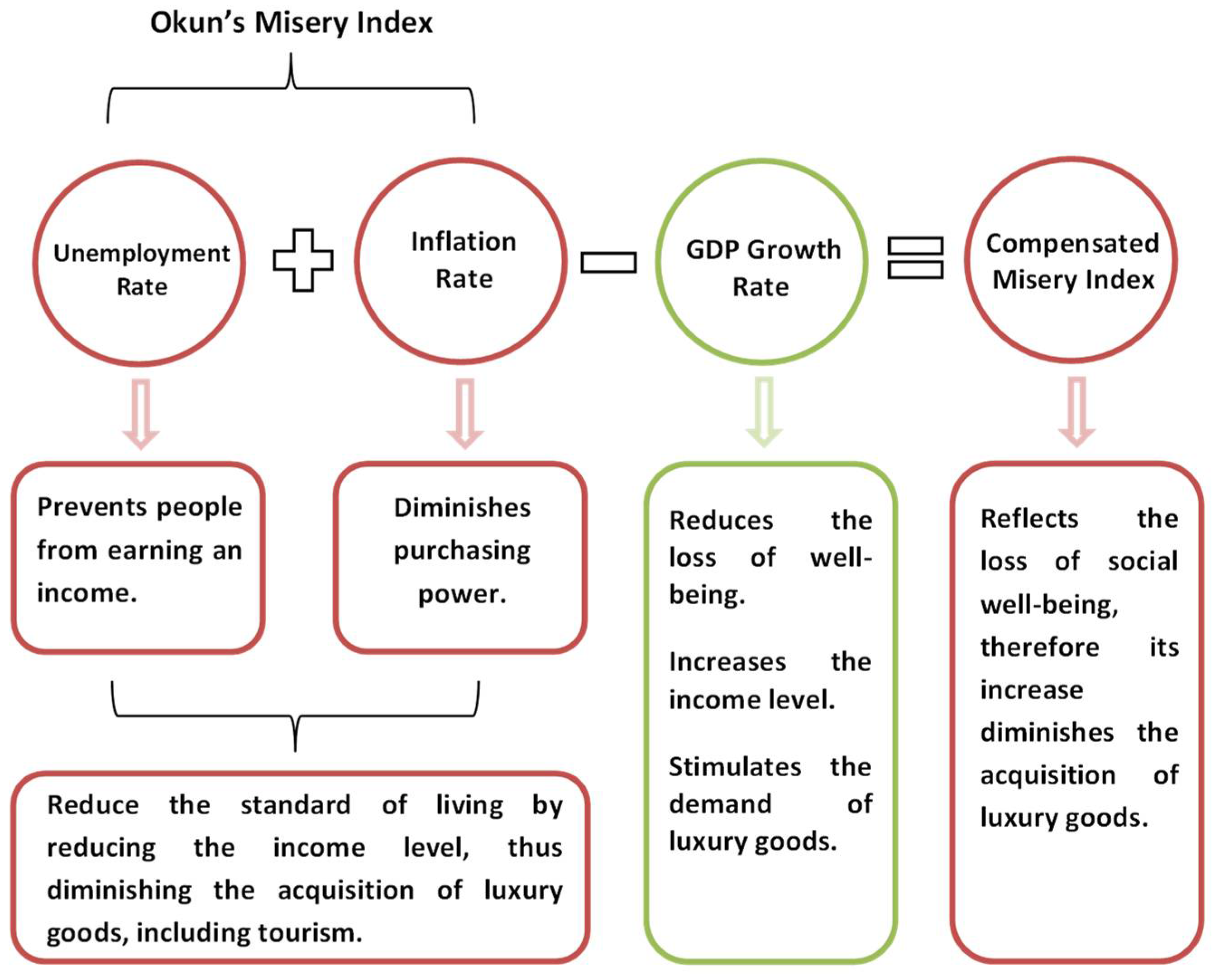
In Figure 1, we summarize the main effects of each CMI component on the consumption of luxury goods and, by extension, on outbound tourism.

It is important to mention that in this literature review we did not find any research on the effect of poverty on international tourist departures. Conversely, there are various studies on the effect of tourism on poverty alleviation in different countries, such as Kenya (Njoya and Seetaram 2018), Mexico (Garza-Rodriguez 2019), and South Africa (Saayman et al. 2012).

3. Materials and Methods

3.1. Data and Sources

To conduct this study, we used time-series data from the second quarter of 2000 to the second quarter of 2020 and retrieved the CMI calculated by Sánchez (2021). We also obtained the real exchange rate (RER) index with respect to 111 countries (year base 1990) (Banco de México 2020b) and Mexico’s international outbound tourists (T) in thousands of people (Banco de México 2020a).

Since Sánchez (2021) reports the CMI as quarterly frequency data, we averaged the real exchange rate index into quarterly data. For its part, the number of outbound tourists was aggregated into quarterly data. We seasonally adjusted both of these series by applying the Census X12 filter, a technique that permits easier identification of trends and atypical data in the series (Pindyck and Rubinfeld 2001) in addition to removing calendar effects (Chatfield 2003).

To avoid finding spurious results when computing the VAR model, we applied the breakpoint unit root test to the series (

Table 1. Breakpoint unit root tests, 2000Q2–2020Q2.

Series	Innovation Outlier				Additive Outlier
	A	B	C	D	A	B	C	D
$\ln T$	−1.499	−3.823	−3.877	−3.195	−1.812	−3.296	−4.282	−6.443 ***
$\ln RER$	−2.594	−3.676	−3.562	−3.460	−2.646	−3.733	−3.664	−3.376
$CMI$	−5.476 ***	−5.520 ***	−5.425 **	−5.576 ***	−5.586 ***	−5.520 ***	−5.795 ***	−6.986 ***
$\dot{t}$	−10.94 ***	−10.87 ***	−10.96 ***	−10.06 ***	−14.24 ***	−11.75 ***	−11.08 ***	−13.25 ***
$\dot{rer}$	−8.396 ***	−8.335 ***	−8.270 ***	−8.465 ***	−8.837 ***	−8.835 ***	−8.659 ***	−8.634 ***

Note: A: intercept only; B: trend and intercept (intercept); C: trend and intercept (trend and intercept); D: trend and intercept (trend); lag length: Schwarz criterion; max. lags = 8; breakpoint selection: Dickey-Fuller min-t; ** and *** denote rejection of the unit root hypothesis at the 5% and 1% significance levels, respectively; symbolization: $\dot{t}=\Delta \ln T$, $\dot{rer}=\Delta \ln RER$.

), since traditional unit root tests could fail in the presence of structural changes (Glynn et al. 2007).

The results of such tests indicate that the CMI is an $I\left(0\right)$ series, whereas the multilateral real exchange rate is an $I\left(1\right)$ series, and the number of outbound tourists mostly behaves as an $I\left(1\right)$ series (Table 1). To avoid obtaining spurious results through the VAR model, in addition to the CMI we used the stationary series $\dot{t}$ and $\dot{rer}$, which represent the first difference of $\ln T$ and $\ln RER$, respectively. Since all three variables in the model are stationary (Table 1), following Enders (2015), there is no need to test for cointegration.

Since the CMI, by definition, is the difference between the MI and the GDP growth rate, as shown in Equation (2), this variable is not properly a series in levels; therefore, it was considered adequate to conduct this study by using differentiated series, and computing a VAR model in differences.

3.2. Empirical Design

A VAR$\left(p\right)$ model including three endogenous variables, two exogenous variables, and a constant, can be written as a system of equations, as shown in Equation (3):

$$\begin{array}{c}\dot{rer}= {\propto }_1+{\displaystyle \sum _{i=1}^p}{\beta }_{1i}{\dot{rer}}_{t-i}+{\displaystyle \sum _{i=1}^p}{\theta }_{1i}CM{I}_{t-i}+{\displaystyle \sum _{i=1}^p}{\gamma }_{1i}{\dot{t}}_{t-i}+{\vartheta }_1{\delta }_{At}+{\mu }_1{\delta }_{Bt}+e_{1t}\\ CMI= {\propto }_2+{\displaystyle \sum _{i=1}^p}{\beta }_{2i}{\dot{rer}}_{t-i}+{\displaystyle \sum _{i=1}^p}{\theta }_{2i}CM{I}_{t-i}+{\displaystyle \sum _{i=1}^p}{\gamma }_{2i}{\dot{t}}_{t-i}+{\vartheta }_2{\delta }_{At}+{\mu }_2{\delta }_{Bt}+e_{2t}\\ \dot{t}= {\propto }_3+{\displaystyle \sum _{i=1}^p}{\beta }_{3i}{\dot{rer}}_{t-i}+{\displaystyle \sum _{i=1}^p}{\theta }_{3i}CM{I}_{t-i}+{\displaystyle \sum _{i=1}^p}{\gamma }_{3i}{\dot{t}}_{t-i}+{\vartheta }_3{\delta }_{At}+{\mu }_3{\delta }_{Bt}+e_{3t}\end{array}$$

(3)

where ${\delta }_A$ is a dummy variable defined to capture the effect of the first COVID-19 wave. COVID-19 was declared a pandemic on 11 March 2020 by the World Health Organization (2020). Following Sáenz (2021), Mexico began to apply sanitary and social distancing measures on 23 March 2020. During the second quarter of 2020, according to Cota (2020), Mexico experienced the greatest registered fall in its GDP as a result of the COVID-19 lockdowns. Meanwhile, ${\delta }_B$ helps the model to adequately simulate the main breaks in the series; that is, the particular periods where the model overestimated or underestimated the series.

$${\delta }_{At}=\{\begin{array}{cc}1& t=2020Q2\\ 0& Otherwise\end{array}$$

(4)

$${\delta }_{Bt}=\{\begin{array}{ccc}1& if t=& 2001Q3;2007Q2;2009Q3;2013Q3;2014Q1\\ -1& if t=& \begin{array}{c}2001Q4;2002Q3;2003Q1;2007Q1;2010Q3;\\ 2017Q1;2018Q3; 2020Q1\end{array}\\ 0& & Otherwise\end{array}$$

(5)

According to Catalán (n.d.), VAR models permit a better understanding of the relations among a set of variables, and, as they are specified without imposing restrictions on the parameters, its specification is more flexible in comparison to other models. Nonetheless, according to Jaramillo (2009), there are several criticisms of VAR models, which are non-parsimonious representations of a time-series vector, leading to problems with degrees of freedom, overfitting, and multicollinearity.

To tackle these eventualities, we first estimated the optimal value for $p$ by using the traditional information criteria: sequential modified LR test statistic (LR), final prediction error (FPE), Akaike (AIC), Schwarz (SIC), and Hannan–Quinn (HQ). As we used quarterly data, we allowed a maximum of six lags when performing this test (

Table 2. VAR lag order selection criteria.

Lag	LR	FPE	AIC	SIC	HQ
0	NA	5.26 × 10−6	−3.641207	−3.360982 *	−3.529422
1	34.13363	4.07 × 10−6	−3.899929	−3.339480	−3.676359 *
2	17.30131	3.99 × 10−6 *	−3.922859 *	−3.082187	−3.587505
3	10.65644	4.30 × 10−6	−3.851494	−2.730598	−3.404355
4	4.865500	5.09 × 10−6	−3.690717	−2.289596	−3.131793
5	19.23276 *	4.67 × 10−6	−3.790916	−2.109571	−3.120207
6	8.597716	5.16 × 10−6	−3.709894	−1.748325	−2.927400

Note: * indicates lag order selected by the criterion.

).

According to the FPE and AIC, the optimal number of lags in this model was $p=2$, whereas the rest of the criteria differed in their number of lags (Table 2). Accordingly, the VAR$\left(2\right)$ was computed.

Concerning multicollinearity, since each equation in a VAR can be individually computed as an ordinary least squares regression (Gujarati and Porter 2009), we computed the variance inflation factors (VIF) to test for multicollinearity.

Finally, the econometric analysis in this study was conducted by means of an unrestricted VAR model, as we have not found empirical or theoretical evidence concerning the relationship between the CMI and the real exchange rate and, as mentioned by Gottschalk (2001), restrictions in a model should not be imposed in the absence of an adequate theoretical framework.

4. Econometric Results

To test the impact of the CMI on Mexican outbound tourism, we performed a VAR$\left(2\right)$, the results of which are summarized in

Table 3. VAR model.

Variable	$\dot{\mathit{r}\mathit{e}\mathit{r}}$	$\mathit{C}\mathit{M}\mathit{I}$	$\dot{\mathit{t}}$
${\dot{rer}}_{t-1}$	0.017232	7.781535	0.178309
	[0.14549]	[2.45109]	[1.71666]
${\dot{rer}}_{t-2}$	0.010501	−0.287187	−0.274804
	[0.08629]	[−0.08804]	[−2.57475]
$CM{I}_{t-1}$	7.37×10−5	0.439408	−0.012036
	[0.01658]	[3.68698]	[−3.08665]
$CM{I}_{t-2}$	−0.002146	0.165540	0.002851
	[−0.51739]	[1.48898]	[0.78369]
${\dot{t}}_{t-1}$	−0.021513	−2.248327	−0.220603
	[−0.24778]	[−0.96606]	[−2.89716]
${\dot{t}}_{t-2}$	−0.116459	3.366115	−0.203880
	[−1.32859]	[1.43263]	[−2.65214]
$Intercept$	0.014092	1.759171	0.054928
	[0.63756]	[2.96921]	[2.83364]
${\delta }_{At}$	0.144122	18.23392	−1.777181
	[3.22700]	[15.2312]	[−45.3734]
${\delta }_{Bt}$	−0.005807	−0.518049	0.115389
	[−0.48615]	[−1.61796]	[11.0148]
$R^2$	0.190572	0.820348	0.971770
$\mathrm{Adjusted} R^2$	0.096725	0.799518	0.968497
F-statistic	2.030669	39.38440	296.8990

Note: [ ] t-statistic.

.

After computing the VAR, we verified that it satisfied the correct specification tests at the 5% significance level (

Table 4. VAR joint correct specification tests.

Test	Statistic	Probability
Doornik–Hansen Normality Test:
Skewness	6.9977	0.0720
Kurtosis	3.5516	0.3141
Jarque–Bera	10.549	0.1033
Serial Correlation LM test (Rao F-statistic):
No serial correlation at lag h (12)	1.7071	0.0915
No serial correlation at lags 1 to h (12)	1.1366	0.2630
White heteroskedasticity test (no cross terms)	102.89	0.1665
White heteroskedasticity test (cross terms)	226.55	0.2975

Note: Tests at the 5% significance level.

). The full serial correlation tests are presented in

Table A1. VAR serial correlation LM test.

	No Serial Correlation at Lag h †				No Serial Correlation at Lags 1 to h †
Lag	LRE Statistic	Probability	Rao F-Statistic	Probability	LRE Statistic	Probability	Rao F-Statistic	Probability
1	9.060541	0.4317	1.013143	0.4319	9.060541	0.4317	1.013143	0.4319
2	7.599082	0.5750	0.845804	0.5752	17.19578	0.5097	0.957877	0.5106
3	8.567566	0.4781	0.956525	0.4783	19.51866	0.8503	0.710730	0.8515
4	6.853486	0.6524	0.761021	0.6525	27.88877	0.8311	0.758812	0.8340
5	14.21805	0.1148	1.616097	0.1149	39.66932	0.6966	0.868085	0.7045
6	5.275074	0.8097	0.582841	0.8098	49.08210	0.6641	0.892998	0.6780
7	11.77062	0.2266	1.327541	0.2267	69.43596	0.2697	1.117055	0.2933
8	4.623273	0.8658	0.509775	0.8659	81.64260	0.2046	1.155866	0.2360
9	5.778344	0.7619	0.639461	0.7620	85.53962	0.3437	1.051483	0.3974
10	13.43430	0.1439	1.523209	0.1441	102.3129	0.1767	1.153246	0.2362
11	7.411738	0.5943	0.824463	0.5945	109.5561	0.2200	1.103615	0.3103
12	14.98239	0.0914	1.707127	0.0915	122.8287	0.1560	1.136641	0.2630

Note: ^† Indicates the null hypothesis.

in Appendix A.

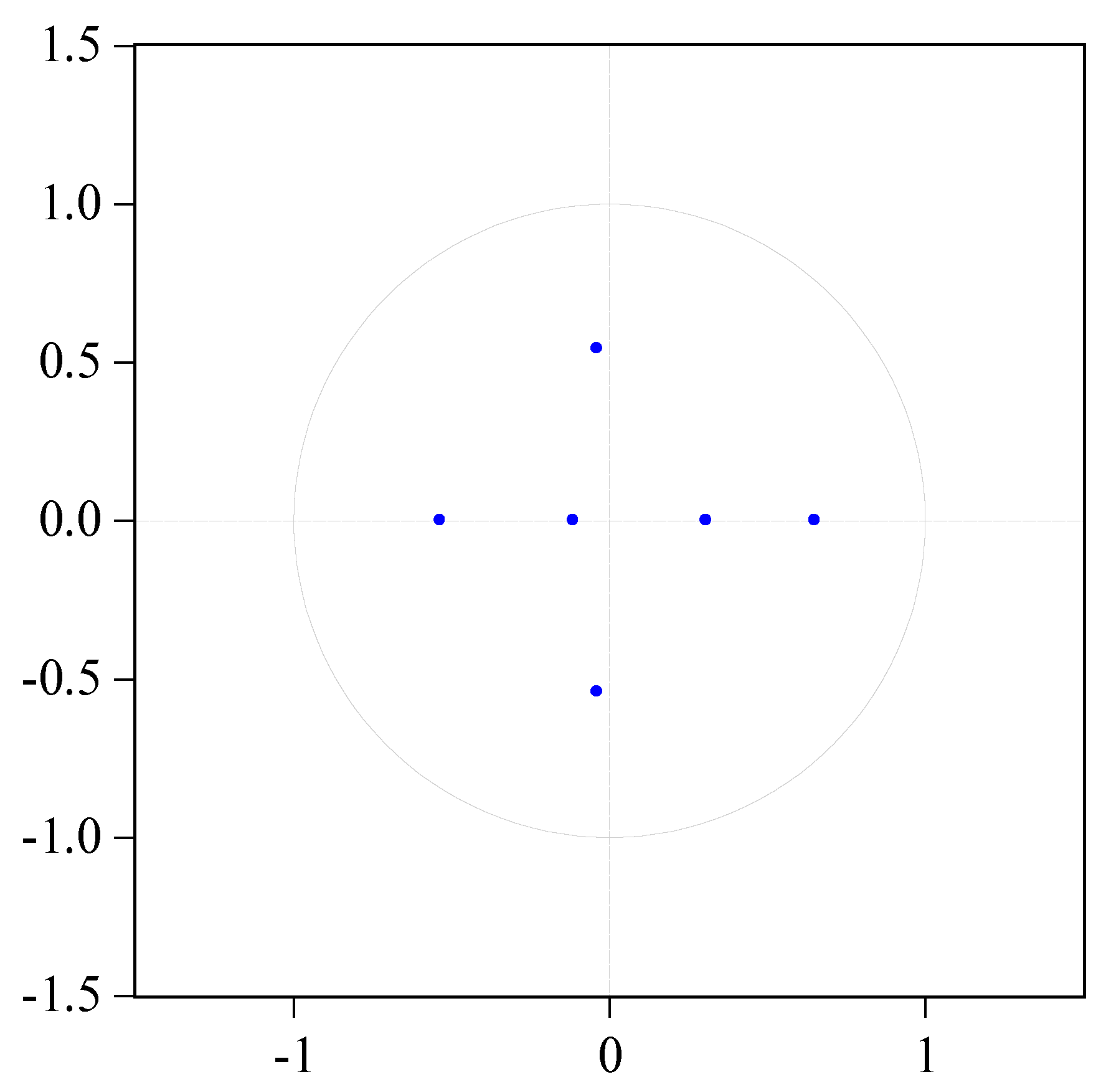
To complement the tests in Table 4, we verified that the model fulfills the stability condition (Figure A1), and, by means of the VIF, we verified that the variables in the model were moderately correlated (

Table A2. Variance Inflation Factors (VIF).

Variable	VIF
${\dot{t}}_{t-1}$	1.224780
${\dot{t}}_{t-2}$	1.139199
${\dot{rer}}_{t-1}$	1.013117
${\dot{rer}}_{t-2}$	1.101008
$CM{I}_{t-1}$	1.469277
$CM{I}_{t-2}$	1.291614
${\delta }_{At}$	1.175898
${\delta }_{Bt}$	1.097881

Note: $1<VIF<5$ indicates moderate correlation. The test does not apply to constants.

).

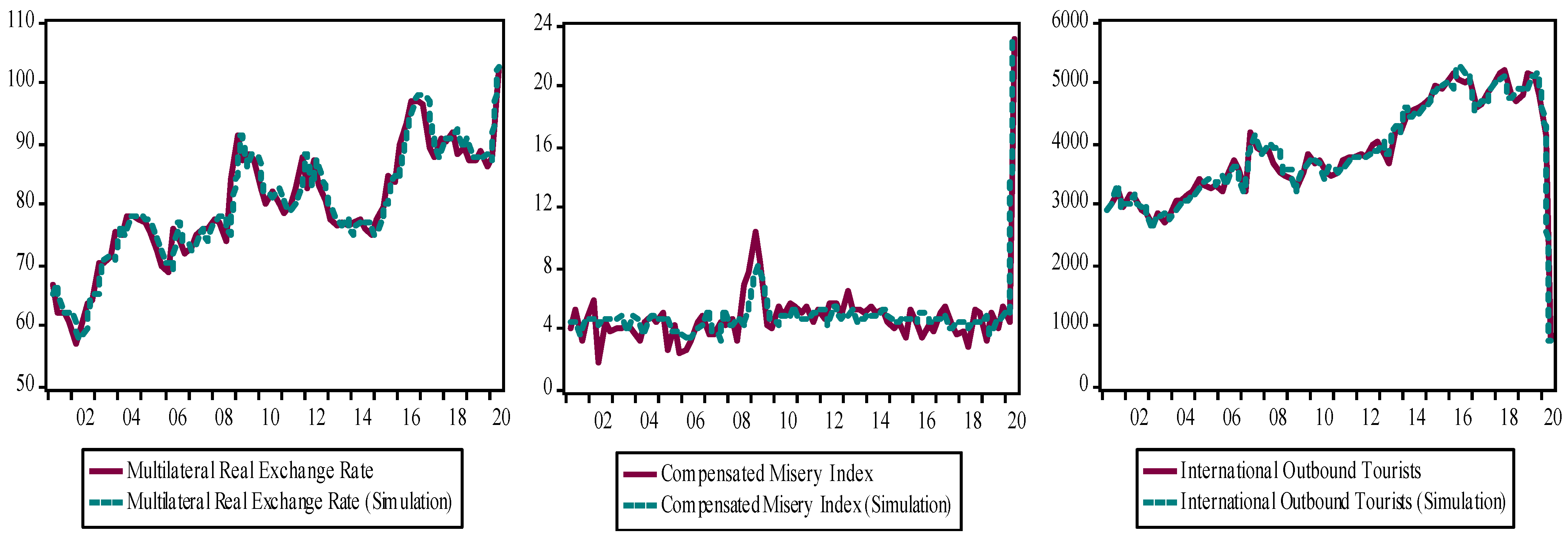
Because the model was computed using the differentiated series $\dot{t}$ and $\dot{rer}$, as a final test for the unrestricted VAR, we tested the model’s capacity to recover the information of these two series in levels, besides correctly simulating the CMI. The results are shown in Figure 2.

As shown in Figure 2, the model satisfactorily simulates the outbound tourism series and identifies the impact of the international financial crisis on the CMI. Additionally, Figure 2 shows that in all three cases the model adequately simulates the second quarter of 2020, which corresponds to the first wave of the COVID-19 pandemic, consistent with the fact that ${\delta }_{At}$ presents the highest t-statistic in all three VAR equations (Table 3). These two facts highlight the importance of introducing dummy variables into the model.

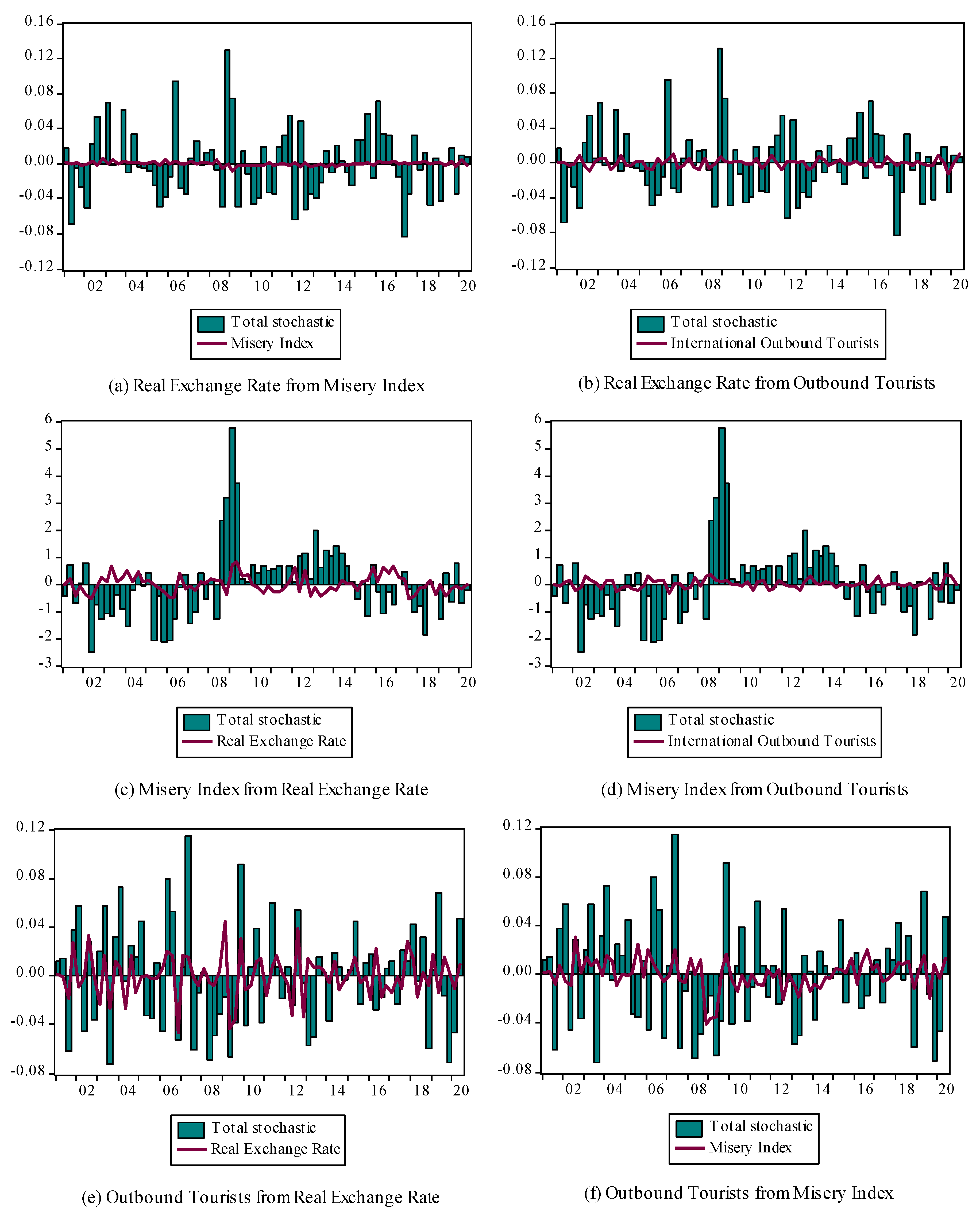
To analyze the model results, we first present a generalized impulse response analysis (Figure 3). The results show that there is no statistically significant response of the multilateral real exchange rate to a shock in the misery index (Figure 3a). Equally, this analysis shows that the multilateral real exchange rate is not significantly affected by shocks in Mexican outbound tourism (Figure 3b).

Concerning the misery index, the impulse response analysis illustrates that it is positively affected by the depreciation of the Mexican peso; this effect is statistically significant during the second period and becomes statistically insignificant during the subsequent periods (Figure 3c). Conversely, an increase in the number of outbound tourists did not significantly affect the CMI (Figure 3d).

In the case of outbound tourists, a depreciation of the Mexican peso reduces the number of tourist departures; such an effect is statistically significant during the third period (Figure 3e). Equally, increases in the CMI diminish the number of outbound tourists; this negative effect is statistically significant only during the second period (Figure 3f).

To gain more statistical evidence supporting the impulse response analysis, we performed the Granger causality test (

Table 5. VAR Granger causality test.

$\mathbf{\text{Dependent Variable: }}\dot{\mathit{r}\mathit{e}\mathit{r}}$
Excluded	χ2	df	Probability
$CMI$	0.317074	2	0.8534
$\dot{t}$	1.776433	2	0.4114
All	1.994013	4	0.7369
$\mathbf{\text{Dependent Variable: }}\mathit{C}\mathit{M}\mathit{I}$
Excluded	χ2	df	Probability
$\dot{rer}$	6.012109	2	0.0495 **
$\dot{t}$	3.992835	2	0.1358
All	9.993396	4	0.0405 **
Dependent Variable: $\dot{\mathit{t}}$
Excluded	χ2	df	Probability
$\dot{rer}$	9.059435	2	0.0108 **
$CMI$	9.852963	2	0.0073 ***
All	24.71084	4	0.0001 ***

Note: ** and *** denote rejection of the null hypothesis at the 5% and 1% significance levels, respectively; df—degrees of freedom.

).

According to the results in Table 5, outbound tourists and CMI do not Granger-cause the multilateral real exchange rate. However, this test, congruent with the impulse response analysis, shows a barely significant relationship at the 5% significance level from the real exchange rate to the CMI. In contrast, the results in Table 5 show that outbound tourism does not Granger-cause CMI, whereas the multilateral real exchange rate and CMI have statistically significant effects on outbound tourism at the 5% and 1% significance levels, respectively.

As a second method to analyze the model’s results, we performed a variance decomposition analysis (

Table 6. Variance decomposition (Cholesky).

Period	$\mathbf{Decomposition} \mathbf{of} \dot{\mathit{r}\mathit{e}\mathit{r}}$			$\mathbf{Decomposition} \mathbf{of} \mathit{C}\mathit{M}\mathit{I}$			$\mathbf{Decomposition} \mathbf{of} \dot{\mathit{t}}$
	$\dot{\mathit{r}\mathit{e}\mathit{r}}$	$\mathit{C}\mathit{M}\mathit{I}$	$\dot{\mathit{t}}$	$\dot{\mathit{r}\mathit{e}\mathit{r}}$	$\mathit{C}\mathit{M}\mathit{I}$	$\dot{\mathit{t}}$	$\dot{\mathit{r}\mathit{e}\mathit{r}}$	$\mathit{C}\mathit{M}\mathit{I}$	$\dot{\mathit{t}}$
1	100.00	0.000	0.000	0.142	99.857	0.000	0.452	0.746	98.800
5	98.715	0.228	1.056	6.899	92.220	0.880	18.503	8.994	72.501
10	98.700	0.237	1.061	7.025	92.099	0.875	18.566	9.063	72.370
15	98.700	0.237	1.062	7.026	92.098	0.875	18.567	9.063	72.369
20	98.700	0.237	1.062	7.026	92.098	0.875	18.567	9.063	72.369

Note: Cholesky ordering: $\dot{rer}$, $CMI$, $\dot{t}$. Only the first three decimal positions are considered in the data.

). Concordant with the previous analyses, variance decomposition shows that CMI and outbound tourism do not make a meaningful contribution to explaining variations in the real exchange rate. More precisely, the CMI explains only 0.23% of the real exchange rate variations, whereas outbound tourism contributes 1.06% to explaining the compensated real exchange rate.

On the other hand, the real exchange rate explains 7.02% of the variations in the CMI during the last period studied. Meanwhile, outbound tourism barely explains 0.87% of the variations in the CMI. Conversely, the real exchange rate contributes 18.56% to an explanation of the changes in outbound tourism once the model is stabilized, whereas CMI explains 0.74% of the changes in Mexican outbound tourism flows during the first period and 9.06% during the last period (Table 6).

As the last method to analyze the VAR results, we performed a historical decomposition analysis (Figure 4). In agreement with the previous analyses, the historical decomposition shows that the real exchange rate is not associated with changes in the CMI (Figure 4a). Equally, the historical decomposition confirms that outbound tourism is not related to the multilateral real exchange rate variations (Figure 4b).

Historical decomposition also reveals that the real exchange rate moderately explains changes in the CMI during three periods: the first and longest was 2004–2006, then during 2009, when the Mexican economy was suffering the adverse effects of the international financial crisis, and finally during 2017–2018. However, this relationship became even weaker or disappeared during the rest of the study period (Figure 4c). Figure 4d shows that outbound tourism does not explain the changes in the compensated misery index.

For its part, the real exchange rate explained the changes in Mexican outbound tourism flows during most of the period studied; the historical decomposition reveals that the real exchange rate was particularly important to explain changes in outbound tourism during 2009 and 2012. Additionally, this analysis shows that the real exchange rate weakly explained outbound tourism during the first COVID-19 wave (Figure 4e).

Finally, Figure 4f shows that CMI was a particularly important variable for understanding the evolution of Mexican outbound tourism flows during the international financial crisis; however, the effect of CMI on outbound tourism became weaker during the subsequent periods, including the first wave of the COVID-19 pandemic.

5. Discussion and Conclusions

In this study, we analyzed the effect of the CMI on the number of international tourist departures from Mexico using a VAR$\left(2\right)$ model, which comprises the period 2000Q2–2020Q2. The CMI was used to approximate the effect of poverty on the number of tourists traveling abroad.

The VAR model results indicate that the multilateral real exchange rate exerted a positive effect on the CMI (Figure 3c) and a negative effect on tourist departures (Figure 3e). In both cases, the effect of multilateral real exchange was stronger during the international financial crisis (Figure 4c,e). Since outbound tourism is considered a type of import, the result in Figure 3e is consistent with economic theory, given that the depreciation of the national currency diminishes the demand for imports (Dornbusch et al. 2002). However, tourist departures had no effect on the CMI (Figure 3d).

On the other hand, the results also indicate that increases in the CMI negatively impact the number of tourist departures (Figure 3f). Figure 4f reveals that CMI was particularly important in explaining the number of outbound tourists during the years of the international financial crisis. Additionally, the CMI explained 9.06% of the variations in the number of tourist departures once the model was stabilized (Table 6).

During 2009, there were substantial increases in the Mexican unemployment rate due to the economic slowdowns over the entire North American region, which considerably diminished the production level of goods and services (Díaz-Bautista 2009). Both of these factors are mirrored in the CMI (Figure 2), leading to a reduction in the demand for outbound tourism.

On the other hand, Figure 4f illustrates that CMI was not closely related to the number of tourist departures during the second quarter of 2020. According to Sigala (2020), the COVID-19 pandemic has had profound negative consequences for tourism, travel, and leisure, as nations implemented strategies such as community lockdowns, stay-at-home campaigns, and self- or mandatory quarantine to prevent new contagions. Additionally, according to the World Bank (2020), the pandemic irrupted mobility, as private or public means of transport were reduced drastically.

In addition to the above-mentioned travel restrictions, two types of fears affecting tourism have been identified as results of the COVID-19 pandemic, namely: fear of lack of enough money for living, and fear of traveling due to the possibility of contagion (Gajić et al. 2021). Both of these fears are strongly related to tourism, since tourism demand is directly related to increases in disposable income, particularly when basic needs have been satisfied (Panosso and Lohmann 2012), and the fear of traveling directly impacts the desire to travel, which is among the main factors that sustain tourism (Ramírez 1994). However, fear of traveling can result from two main circumstances: direct experience or indirect affectation by events abroad due to the information received from a reference group; therefore, tourist behavior during crises can be considered heterogeneous rather than homogeneous (Çakar 2021).

According to Cerón (2020), the COVID-19 pandemic has caused numerous potential outbound tourists to change their travel plans for domestic travels, which has also been a response to labor instability. In this sense, according to the same author, it is important that tourist destinations that have traditionally focused on receiving international tourists redirect their strategies to attract a higher number of domestic tourists.

In Mexico, the internal control of the pandemic allowed the country to reach an unusually high position in the ranking of the most visited countries. Effectively, Weiss (2021) reports that Mexico was the third most visited country during 2020, since the country never closed its frontiers, and is among the few nations that do not require a negative COVID-19 test to enter. Moreover, Paredes (2022) reports that Mexico could become the second most visited nation due to the 31.9 million international tourists who visited the country during 2021. However, Paredes mentions that once travel conditions are normalized, Mexico will probably occupy the same position it did prior to the pandemic.

Although the negative effects of the COVID-19 pandemic on tourism seem to be deeper than those occasioned by previous pandemics (Škare et al. 2021), the pandemic has brought a new form of tourism, the so-called “vaccine tourism”, which, according to Şengel (2021), consists of travel by people who cannot get vaccinated in their own country or who do not want to wait for their turn to be vaccinated. However, Şengel points out that this new type of tourism commoditizes vaccination as another tourist attraction. In the case of Mexico, outbound tourism has been revitalized by this new form of tourism, since Guillén (2021) reports that between March and May 2021, trips made by Mexicans to the United States grew substantially because of the COVID-19 vaccine, reaching 905,487, whereas in the previous three months only 380,000 trips to the U.S. were registered.

However, there was a negative relationship between the CMI and tourist departures during the study period (Figure 3f). In light of the model’s results, and given that all three CMI components are related to tourist departures, observing the evolution of the CMI of the main countries of origin of travelers could help to predict decreases in the arrival of international tourists, allowing the implementation of adequate policies to address the decrease in tourism demand.

Different measures to tackle the decline in the tourism sector have been suggested: the main strategies, following the OECD (2020), are restoring traveler confidence, promoting domestic tourism, supporting the safe return of international tourism, and strengthening cooperation within and between countries. The correct implementation of these policies is essential in a context where tourism has undergone one of its deepest crises. Considering that many people have experienced economic difficulties during the pandemic, such policies could be strengthened by tourism service providers by offering attractive all-inclusive packages, limited-time discounts, and, more importantly, offering safe tourist spaces.

Finally, according to Blišt’anová et al. (2021), there have also been numerous precautionary measures undertaken by airports to prevent the virus from spreading, for example: negative COVID-19 tests, the use of face masks, temperature checks, and health declarations. Consequently, according to the International Civil Aviation Organization (2021), there was a sharp reduction in both domestic and international air traffic. The ICAO recommends focusing on providing safety, security, and efficiency. It is very important to mention that the ICAO recommends that all future restrictions implementation to prevent new contagions need to be supported by medical evidence.

References

1. Akçay, Selçuk. 2017. Remittances and misery index in Turkey: Is there a link? Applied Economics Letters 25: 895–99. [Google Scholar] [CrossRef]
2. Alegre, Joaquín, Llorenç Pou, and Maria Sard. 2019. High unemployment and tourism participation. Current Issues in Tourism 22: 1138–49. [Google Scholar] [CrossRef]
3. Álvarez, Pablo. 1996. La relación de los servicios y el turismo con el sector externo en México. Comercio Exterior 46: 148–57. [Google Scholar]
4. Ascanio, Alfredo. 2012. Teoría del Turismo. Mexico: Trillas. [Google Scholar]
5. Asher, Martin A., Robert H. Defina, and Kishor Thanawala. 1993. The misery index: Only part of the story. Challenge 36: 58–62. [Google Scholar] [CrossRef]
6. Banco de México. 2020a. Cuenta de Viajeros Internacionales, Número de Viajeros, Egresos. Available online: https://www.banxico.org.mx/SieInternet/consultarDirectorioInternetAction.do?accion=consultarCuadro&idCuadro=CE36&locale=es (accessed on 12 December 2020).
7. Banco de México. 2020b. Índice de Tipo de Cambio Real con Precios Consumidor y con Respecto a 111 Países. Available online: https://www.banxico.org.mx/SieInternet/consultarDirectorioInternetAction.do?sector=6&accion=consultarCuadro&idCuadro=CR60&locale=es (accessed on 12 December 2020).
8. Barro, Robert J. 1999. Reagan vs. Clinton: Who’s the Economic Champ? Business Week. Available online: https://scholar.harvard.edu/barro/publications/reagan-vs-clinton-whos-economic-champ (accessed on 15 February 2022).
9. Blišt’anová, Monika, Michaela Tirpáková, and L’ubomíra Brůnová. 2021. Overview of Safety Measures at Selected Airports during the COVID-19 Pandemic. Sustainability 13: 8499. [Google Scholar] [CrossRef]
10. Boullón, Roberto C. 2009. Las Actividades Turísticas y Recreacionales: El Hombre como Protagonista. Mexico: Trillas. [Google Scholar]
11. Çakar, Kadir. 2021. Tourophobia: Fear of travel resulting from man-made or natural disasters. Tourism Review 76: 103–24. [Google Scholar] [CrossRef]
12. Catalán, Horacio. n.d. Curso: Econometría y Análisis de Políticas Fiscales. Especificación de los Modelos VAR. CEPAL. Available online: https://www.cepal.org/sites/default/files/courses/files/hc_3_especificacion_var.pdf (accessed on 15 February 2022).
13. Cerón, Hazael. 2020. El turismo doméstico como base de la recuperación post COVID-19 de la actividad turística en México. Revista Latinoamericana de Investigación Social 3: 72–79. [Google Scholar]
14. Chatfield, Chris. 2003. The Analysis of Time Series: An Introduction. New York: Chapman & Hall/CRC. [Google Scholar] [CrossRef]
15. Cohen, Ivan K., Fabrizio Ferretti, and Bryan McIntosh. 2014. Decomposing the misery index: A dynamic approach. Cogent Economics & Finance 2: 991089. [Google Scholar] [CrossRef]
16. Cota, Isabella. 2020. La Economía Mexicana se desploma un 17.3% en el Segundo Trimestre de 2020, la peor Caída de su Historia. El País. Available online: https://elpais.com/mexico/economia/2020-07-30/la-economia-mexicana-se-desploma-un-173-en-el-segundo-trimestre-de-2020-la-peor-caida-de-su-historia.html (accessed on 6 March 2022).
17. Dahdá, Jorge. 2003. Elementos de Turismo: Economía, Comunicación, Alimentos y Bebidas, Líneas Aéreas, Hotelería, Relaciones Públicas. Mexico: Trillas. [Google Scholar]
18. Di Tella, Rafael, Robert J. MacCulloch, and Andrew J. Oswald. 2001. Preferences over inflation and unemployment: Evidence from surveys of happiness. American Economic Review 91: 335–41. [Google Scholar] [CrossRef]
19. Díaz-Bautista, Alejandro. 2009. La crisis económica del 2009, las remesas y el desempleo en el área del TLCAN. Ra Ximhai 5: 39–48. [Google Scholar] [CrossRef]
20. Dominé, Rolando A. 2014. Las Variables Económicas que más Afectan las Decisiones de Viajes. Universidad FASTA. Available online: https://www.ufasta.edu.ar/noticias/files/2014/04/FASTA-NEWSLETTERS-Turismo-y-Variables-econ%C3%B3micas-04-2014-Domin%C3%A9.pdf (accessed on 10 February 2022).
21. Dornbusch, Rudiger, Stanley Fischer, and Richard Startz. 2002. Macroeconomía. Madrid: McGraw-Hill. [Google Scholar]
22. Enders, Walter. 2015. Applied Econometric Time Series. Hoboken: Wiley. [Google Scholar]
23. Gaddo, Filippo. 2011. An International Analysis of the Misery Index. Londra: Fondazione Magna Carta. [Google Scholar]
24. Gajić, Tamara, Marko D. Petrović, Ivana Blešić, Milan M. Radovanović, and Julia A. Syromiatnikova. 2021. The power of fears in the travel decision—COVID-19 against lack of money. Journal of Tourism Futures, 1–22. [Google Scholar] [CrossRef]
25. Garza-Rodriguez, Jorge. 2019. Tourism and poverty reduction in Mexico: An ARDL cointegration approach. Sustainability 11: 845. [Google Scholar] [CrossRef] [Green Version]
26. Glynn, John, Nelson Perera, and Reetu Verma. 2007. Unit root tests and structural breaks: A survey with applications. Revista de Métodos Cuantitativos para la Economía y la Empresa 3: 63–79. [Google Scholar]
27. Gottschalk, Jan. 2001. An Introduction into the SVAR Methodology: Identification, Interpretation and Limitations of SVAR Models. Kiel Working Paper No. 1072. Available online: https://www.files.ethz.ch/isn/124218/kap1072.pdf (accessed on 8 March 2022).
28. Grabia, Tomasz. 2011. The Okun misery index in the European Union countries from 2000 to 2009. Comparative Economic Research. Central and Eastern Europe 14: 97–115. [Google Scholar] [CrossRef]
29. Guillén, Beatriz. 2021. El Turismo de Vacunación contra la COVID-19 Triplica los Viajes de Mexicanos a Estados Unidos. El País. Available online: https://elpais.com/mexico/2021-07-16/el-turismo-de-vacunacion-contra-la-covid-19-triplica-los-viajes-de-mexicanos-a-estados-unidos.html (accessed on 15 February 2022).
30. Gujarati, Damodar N., and Dawn C. Porter. 2009. Econometría. Mexico: McGraw-Hill. [Google Scholar]
31. Hipsher, Scott. 2017. Tourism: Job creation, entrepreneurship, and quality of life. In Poverty Reduction, the Private Sector, and Tourism in Mainland Southeast Asia. Singapore: Palgrave Macmillan, pp. 231–51. [Google Scholar] [CrossRef]
32. Hortalà, Joan, and Damià Rey. 2011. Relevancia del índice de malestar económico. Cuadernos de Economía 34: 162–69. [Google Scholar] [CrossRef] [Green Version]
33. International Civil Aviation Organization (ICAO). 2021. Take-Off: Guidance for Air Travel through the COVID-19 Public Health Crisis. Available online: https://www.icao.int/COVID/cart/Documents/CART%20III_Take-off%20Guidance%20for%20Air%20Travel%20through%20the%20COVID-19%20Public%20Health%20Crisis.en.pdf (accessed on 8 March 2022).
34. Jaramillo, Patricio. 2009. Estimación de VAR Bayesianos para la economía chilena. Revista de Análisis Económico 24: 101–26. [Google Scholar]
35. Kim, Hong-bumm, Jung-Ho Park, Seul Ki Lee, and SooCheong (Shawn) Jang. 2012. Do expectations of future wealth increase outbound tourism? Evidence from Korea. Tourism Management 33: 1141–47. [Google Scholar] [CrossRef] [PubMed]
36. Lechman, Ewa. 2009. Okun’s and Barro’s Misery Index as an Alternative Poverty Assessment Tool. Recent Estimations for European Countries. MPRA Paper No. 37493. Available online: http://mpra.ub.uni-muenchen.de/37493/ (accessed on 15 February 2022).
37. Lovell, Michael C., and Pao-Lin Tien. 2000. Economic discomfort and consumer sentiment. Eastern Economic Journal 26: 1–8. [Google Scholar] [CrossRef] [Green Version]
38. MacRae, C. Duncan. 1977. A political model of the business cycle. Journal of Political Economy 85: 239–63. [Google Scholar] [CrossRef]
39. Mehran, Javaneh, and Hossein G. T. Olya. 2019. Progress on outbound tourism expenditure research: A review. Current Issues in Tourism 22: 2511–37. [Google Scholar] [CrossRef]
40. Murphy, Ryan H. 2016. A short empirical note on state misery indexes. Journal of Regional Analysis and Policy 46: 186–89. [Google Scholar]
41. Njoya, Eric Tchouamou, and Neelu Seetaram. 2018. Tourism contribution to poverty alleviation in Kenya: A dynamic computable general equilibrium analysis. Journal of Travel Research 57: 513–24. [Google Scholar] [CrossRef] [PubMed] [Green Version]
42. OECD. 2020. Mitigating the Impact of COVID-19 on Tourism and Supporting Recovery. OECD Tourism Papers N° 2020/03. Paris: OECD Publishing. [Google Scholar] [CrossRef]
43. Özcan, Süleyman Emre, and Sezgin Açıkalın. 2015. Relationship between misery index and lottery games: The case of Turkey. International Journal of Humanities and Social Science 5: 159–64. [Google Scholar]
44. Panosso, Alexandre, and Guilherme Lohmann. 2012. Teoría del Turismo: Conceptos, Modelos y Sistemas. Mexico: Trillas. [Google Scholar]
45. Paredes, Miriam. 2022. México es el Segundo País del Mundo que más atrajo Turistas Internacionales en 2021. Dinero en Imagen. Available online: https://www.dineroenimagen.com/actualidad/mexico-es-el-segundo-pais-del-mundo-que-mas-atrajo-turistas-internacionales-en-2021 (accessed on 4 March 2022).
46. Pindyck, Robert S., and Daniel L. Rubinfeld. 2001. Econometría: Modelos y Pronósticos. Mexico: McGraw-Hill. [Google Scholar]
47. Piraee, Khosrow, and Maryam Barzegar. 2011. The relationship between the misery index and crimes: Evidence from Iran. Asian Journal of Law and Economics 2: 1–19. [Google Scholar] [CrossRef]
48. Ramírez, César. 1994. La Modernización y Administración de Empresas Turísticas. Mexico: Trillas. [Google Scholar]
49. Ramoni-Perazzi, Josefa, and Giampaolo Orlandoni-Merli. 2013. El índice de miseria corregido por informalidad: Una aplicación al caso de Venezuela. Ecos de Economía 17: 29–49. [Google Scholar] [CrossRef]
50. Rasool, Haroon, Shafat Maqbool, and Md Tarique. 2021. The relationship between tourism and economic growth among BRICS countries: A panel cointegration analysis. Future Business Journal 7: 1–11. [Google Scholar] [CrossRef]
51. Riascos, Julio C. 2009. El índice de malestar económico o índice de miseria de Okun: Breve análisis de casos. 2001–2008. Tendencias 10: 92–124. [Google Scholar]
52. Saayman, Melville, Riaan Rossouw, and Waldo Krugell. 2012. The impact of tourism on poverty in South Africa. Development Southern Africa 29: 462–87. [Google Scholar] [CrossRef]
53. Sáenz, Claudia. 2021. ‘Línea de Tiempo COVID-19’; A un Año del Primer Caso en México. Secretaría de Cultura—Gobierno de la Ciudad de México. Available online: https://www.capital21.cdmx.gob.mx/noticias/?p=12574 (accessed on 6 March 2022).
54. Sánchez, Fernando. 2019. Unemployment and growth in the tourism sector in Mexico: Revisiting the growth-rate version of Okun’s Law. Economies 7: 83. [Google Scholar] [CrossRef] [Green Version]
55. Sánchez, Fernando. 2021. International visitors and misery index in Mexico. Mendeley Data. [Google Scholar] [CrossRef]
56. Seetaram, Neelu. 2010. A Study on Outbound Tourism from Australia. Discussion Paper 47/10. Narre Warren: Monash University, Available online: https://www.monash.edu/__data/assets/pdf_file/0005/925457/a_study_of_outbound_tourism_from_australia.pdf (accessed on 15 February 2022).
57. Şengel, Ümit. 2021. From crisis to opportunity: “Vaccine Tourism”. Turizm ve İşletme Bilimleri Dergisi 1: 51–56. [Google Scholar]
58. Sharma, A., and M. Thapar. 2016. Development of tourism in the Third World nations: A comparative analysis. In Sustainable Tourism VII. Southampton: WIT Press, pp. 155–66. [Google Scholar] [CrossRef] [Green Version]
59. Sigala, Marianna. 2020. Tourism and COVID-19: Impacts and implications for advancing and resetting industry and research. Journal of Business Research 117: 312–21. [Google Scholar] [CrossRef] [PubMed]
60. Škare, Marinko, Domingo Riberio, and Małgorzata Porada-Rochoń. 2021. Impact of COVID-19 on the travel and tourism industry. Technological Forecasting & Social Change 163: 120469. [Google Scholar] [CrossRef]
61. Smeral, Egon. 2003. A structural view of tourism growth. Tourism Economics 9: 77–93. [Google Scholar] [CrossRef]
62. Sosa, Sergio W. 2001. Modelos Macroeconómicos: De los “Clásicos” a la Macroeconomía de las Economías Periféricas. Mexico: Tlaxcallan. [Google Scholar]
63. Stabler, Mike J., Andreas Papatheodorou, and M. Thea Sinclair. 2009. The Economics of Tourism. London: Routledge. [Google Scholar] [CrossRef]
64. Varian, Hal R. 1999. Microeconomía Intermedia: Un Enfoque Actual. Barcelona: Antoni Bosch. [Google Scholar]
65. Wang, Nianyong, Muhammad Haroon Shah, Kishwar Ali, Shah Abbas, and Sami Ullah. 2019. Financial structure, misery index, and economic growth: Time series empirics from Pakistan. Journal of Risk and Financial Management 12: 100. [Google Scholar] [CrossRef] [Green Version]
66. Weinz, Wolfgang, and Lucie Servoz. 2013. Poverty Reduction through Tourism. Geneva: International Labour Office. [Google Scholar]
67. Weiss, Sandra. 2021. México brilla como destino turístico, pese al COVID-19. Deutsche Welle. Available online: https://www.dw.com/es/m%C3%A9xico-brilla-como-destino-tur%C3%ADstico-pese-al-covid-19/a-56593033 (accessed on 15 February 2022).
68. Welsch, Heinz. 2007. Macroeconomics and life satisfaction: Revisiting the “misery index”. Journal of Applied Economics 10: 237–51. [Google Scholar] [CrossRef] [Green Version]
69. Winkelmann, Liliana, and Rainer Winkelmann. 1998. Why are the unemployed so unhappy? Evidence from panel data. Economica 65: 1–15. [Google Scholar] [CrossRef] [Green Version]
70. World Bank. 2020. Poverty and Distributional Impacts of COVID-19: Potential Channels of Impact and Mitigating Policies. Available online: https://thedocs.worldbank.org/en/doc/980491587133615932-0090022020/original/PovertyanddistributionalimpactsofCOVID19andpolicyoptions.pdf (accessed on 15 February 2022).
71. World Bank. 2021. International Tourism, Number of Departures. TCdata360. Available online: https://tcdata360.worldbank.org/indicators/ST.INT.DPRT?country=BRA&indicator=1842&viz=line_chart&years=1995,2018 (accessed on 15 February 2022).
72. World Health Organization. 2020. WHO Director-General’s Opening Remarks at the Media Briefing on COVID-19, March 11. Available online: https://www.who.int/director-general/speeches/detail/who-director-general-s-opening-remarks-at-the-media-briefing-on-COVID-19---11-march-2020 (accessed on 6 March 2022).
73. Yang, Bijou, and David Lester. 1999. The misery index and suicide. Psychological Reports 84: 1086. [Google Scholar] [CrossRef] [PubMed]
Figure 1. CMI and tourism.
Economies 10 00081 g001
Figure 2. Unrestricted VAR simulation (Broyden’s algorithm).
Economies 10 00081 g002
Figure 3. Response to generalized one S.D. innovations ± 2 S.E.
Economies 10 00081 g003
Figure 4. Historical decomposition using generalized weights.
Economies 10 00081 g004